Article

Temporal and Spatial Variability of Hydrogeomorphological Attributes in Coastal Wetlands—Lagoa do Peixe National Park, Brazil

by
Carina Cristiane Korb
1,*,
Laurindo Antonio Guasselli
1,*,
Heinrich Hasenack
2,
Tássia Fraga Belloli
1 and
Christhian Santana Cunha
1
1
Laboratory of Geoprocessing and Environmental Analysis (LAGAM), Institute of Geosciences, Postgraduate Program in Remote Sensing, Federal University of Rio Grande do Sul (UFRGS), Porto Alegre 91509-900, Rio Grande do Sul, Brazil
2
Institute of Biosciences, Ecology Center, Federal University of Rio Grande do Sul (UFRGS), Porto Alegre 91540-000, Rio Grande do Sul, Brazil
*
Authors to whom correspondence should be addressed.
Coasts 2025, 5(3), 23; https://doi.org/10.3390/coasts5030023
Submission received: 8 May 2025 / Revised: 20 June 2025 / Accepted: 1 July 2025 / Published: 9 July 2025

Abstract

Coastal wetlands play important environmental roles. However, their hydrogeomorphological dynamics remain poorly understood under scenarios of extreme climate events. The aim of this study was to characterize the temporal and spatial variability of hydrogeomorphological attributes (vegetation, water, and soil) in the wetlands of Lagoa do Peixe National Park, Brazil. The methodology involved applying Principal Component Analysis (PCA) in both temporal (T) and spatial (S) modes, decomposing spectral indices for each attribute to identify variability patterns. The results revealed that vegetation and water are strongly correlated with seasonal dynamics influenced by ENSO (El Niño/La Niña) events. Soils reflected their textural characteristics, with a distinct temporal response to the water balance. PCA proved to be a useful tool for synthesizing large volumes of multitemporal data and detecting dominant variability patterns. It highlighted the Lagoon Terraces and the Lagoon Fringe, where low slopes amplified hydrological variations. Temporal variability was more responsive to climate extremes, with implications for ecosystem conservation, while spatial variability was modulated by geomorphology.

1. Introduction

Coastal wetlands play a fundamental role in providing habitats, mitigating floods [1,2,3], and in carbon sequestration and storage [4,5,6], contributing approximately 12% to the global carbon stock [7]. In addition to their ecological value, these areas have high economic importance [8], playing a key role in both environmental and socioeconomic sustainability.
Despite their importance, studies warn of the accelerated degradation of these ecosystems, with estimated losses ranging from 21% to 35% between 1700 and 2020 [9,10,11,12], and a 47% reduction in Ramsar sites between 1980 and 2014 [13]. Global wetland area estimates vary from 0.54 to 21.26 million km2, but the specific spatial consistency for the wetlands class is below 1% [14]. However, variations among estimates may partly reflect differences in wetland definitions. The conservation of these environments is emphasized in international agreements such as the Ramsar Convention and the Kyoto Protocol [9], and is also considered strategic for achieving the Sustainable Development Goals [15].
The dynamics of coastal wetlands are characterized by high spatiotemporal complexity, resulting from the interaction among morphology, soils, vegetation, and hydrological pulses [16,17,18]. These processes vary across different hydrogeomorphological compartments and are modulated by seasonal and interannual climatic factors, such as El Niño and La Niña events [17], which affects hydrological connectivity [17,19]. Landscape pattern changes, intensified by coastal winds and sea level fluctuations, make these areas particularly sensitive to environmental disturbances [18,19,20,21,22].
The delineation and interpretation of the temporal and spatial variability of wetlands through remote sensing are challenging [2]. In coastal wetlands, water level fluctuations [23], the spectral similarity of vegetation [24], the presence of hydromorphic soils [25], and the very flat topography of coastal areas [17] complicate compartmentalization and zoning efforts. Spectral mixing of vegetation and water content hinders the use of traditional approaches for wetland classification and mapping [26], requiring multiscale methods capable of synthesizing complex and multivariate spatiotemporal patterns [27]. Moreover, freely available elevation data are not sufficiently accurate to model coastal environments with very small altimetric variation [28].
In this context, Principal Component Analysis (PCA) has proven to be a useful tool for synthesizing large volumes of multitemporal data and detecting dominant patterns of variability, as it reduces data dimensionality [29,30]. Although PCA has already been applied in inland wetlands, such as the Brazilian Pantanal [31,32], southern Zambia [33], and the coast of Mexico [34,35], its use in subtropical coastal wetlands remains incipient. However, conventional PCA approaches present limitations when applied to environments with high spectral redundancy, as is the case with wetlands.
To overcome these limitations, this study adopts PCA in T-mode (temporal) and S-mode (spatial), which enables the investigation of recurring temporal and spatial patterns of environmental variability throughout the historical series [29,30,36]. This approach has been successfully applied in coastal areas of Mexico [35] and China [37], demonstrating its applicability for the integrated analysis of environmental dynamics. Based on data variance, PCA in T- and S-modes reduces redundancy in multispectral datasets and allows for the identification of main spatial patterns, facilitating the interpretation of systemic processes [30].
In the Lagoa do Peixe National Park (PNLP), an important Ramsar Site in southern Brazil, environmental dynamics are strongly influenced by its low elevation relative to sea level and the occurrence of extreme events associated with the El Niño, Southern Oscillation, and the Southern Hemisphere Annular Mode [17,22]. Studies in the region have contributed to the understanding of the biota [38,39,40], as well as geology, geomorphology, and climatology [41,42,43,44,45], the dynamics of flood pulses [46] and hydrogeomorphological compartments [17]. However, the temporal and spatial variability of hydrogeomorphological attributes, particularly vegetation, water, and soils, remains poorly understood and difficult to classify using traditional methods.
Thus, this study aims to characterize the temporal and spatial variability of hydrogeomorphological attributes of the coastal wetlands in PNLP, using spectral indices representative of vegetation, water, and soil through the application of PCA in T and S modes. The adopted approach helps to fill a knowledge gap regarding the hydrogeomorphological dynamics of these ecosystems in the South American subtropical context, providing a solid methodological foundation for future monitoring and conservation studies.

2. Materials and Methods
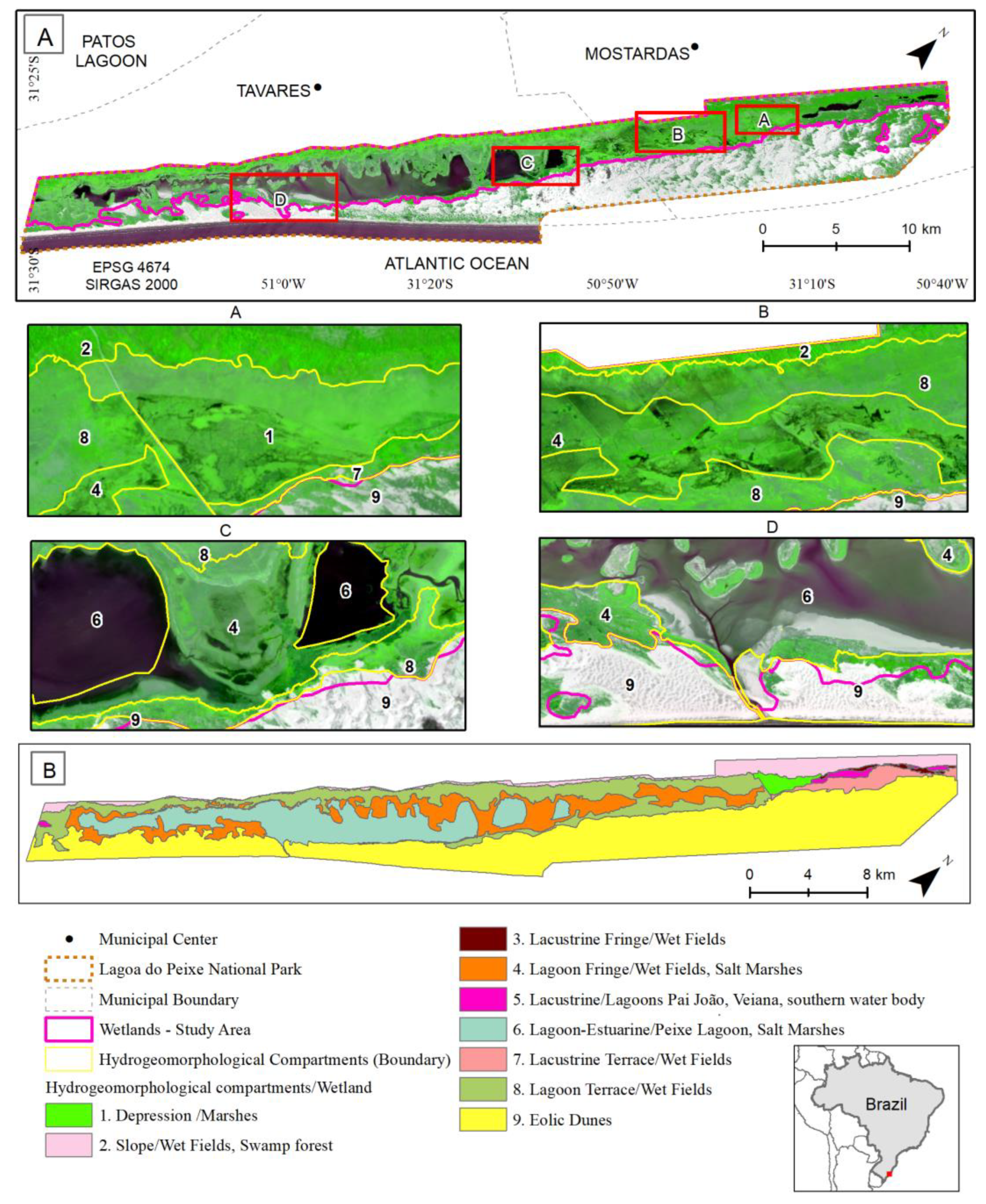
2.1. Study Area

In Brazil, coastal wetlands are distributed along the entire coastline, encompassing both the tropical and subtropical zones. They include a wide variety of ecosystems, such as dunes, restingas, sandy beaches, rocky shores, lagoons, estuaries, salt marshes, mangroves, and coral reefs [47].
In the extreme south of Brazil, the Coastal Plain of the state of Rio Grande do Sul (PCRS) has recorded four episodes of transgression and regression during the Quaternary period, which led to the formation of four depositional systems known as the Laguna-Barreira System: three from the Pleistocene epoch (I, II, and III) and one from the Holocene (IV) [48,49,50]. Due to its morphogenesis, the PCRS harbors the highest concentration of coastal wetlands [51]. However, between 1985 and 2021, changes in land use and land cover revealed extensive suppression of wetland areas, impacting the extent and dynamics of these ecosystems [52].
The Lagoa do Peixe National Park (PNLP) is located in the middle section of the Coastal Plain of Rio Grande do Sul (PCRS), between the Patos Lagoon and the Atlantic Ocean, within the municipalities of Tavares and Mostardas (Figure 1). It is a fully protected Conservation Unit, established in 1986. Due to its importance for the conservation of coastal ecosystems and migratory bird habitats, it was designated as a Ramsar Site in 1993. Currently, the park is part of the Atlantic Forest Biosphere Reserve and the Western Hemisphere Shorebird Reserve Network [53,54]. Coastal wetlands cover approximately 47% of the Park’s area, and Lagoa do Peixe, the main water body, periodically connects with the ocean [44].
Five geological-geomorphological features occur within the park: the Paleocliff of Barrier III, Colluvial Deposits of Barrier III, Lagoon Terrace I, Lagoon Terrace II, and Eolic Dunes of Barrier [41]. The highest elevations are found in the Paleocliff of Barrier III and the Eolic Dunes of Barrier IV [17,22]. The overall morphology consists of an extensive sandy plain, with flat topography and low elevation relative to sea level (Figure 2A). Wetlands occupy the interdune spaces, the areas between the lagoon terraces, and parts of the colluvial deposits of Barrier III. They are present across all hydrogeomorphological compartments, except in the Eolic Dunes, where wind conditions do not favor their formation and persistence. These areas are highly susceptible to flooding pulses associated with extreme precipitation events.
Nine hydrogeomorphological compartments occur in the area (Figure 1B): Eolic Dunes, Lagoon Fringe, Lacustrine Fringe, Lacustrine, Lagoon-Estuarine, Lacustrine Terrace, Lagoon Terrace, Depression, and Slope [17]. The dominant soil type is Melanic Gleysol, a hydromorphic soil developed from recent, unconsolidated Holocene sediments, with clayey, clay-sandy, and sandy textures [57].
The vegetation cover consists of Pioneer Formations or Restinga [50], influenced by both marine and lacustrine conditions. The area features wet grasslands, swamp forests, marshes, tidal flats, and lagoonal water bodies (Figure 2B–D). Additionally, areas of Pinus spp. plantations, considered an invasive species, are spreading over the Park’s sandy terrains [58], affecting the natural stability of the dunes and causing wetland siltation [59].
Annual rainfall in the region ranges between 1200 and 1500 mm, with higher totals occurring during winter and spring, occasionally exceeding the historical average. Precipitation is mainly driven by frontal rainfall resulting from the interaction between Tropical Maritime (mT) and Polar Maritime (mP) air masses, as well as by anomalies associated with large-scale climate phenomena such as the El Niño-Southern Oscillation (ENSO) and the Southern Annular Mode (SAM) [44,60]. El Niño events typically cause above-average rainfall, while La Niña events lead to negative anomalies, significantly reducing water levels in Lagoa do Peixe [42,61,62,63].

2.2. Data and Procedures

This study adopted the following cartographic bases: (a) geomorphological compartments [41]; hydrogeomorphological compartments [17]; (c) wetland mapping by the Zoobotanical Foundation of Rio Grande do Sul [51]; precipitation data from the Climate Hazards Group InfraRed Precipitation with Stations (CHIRPS) product, using Java Script based code structures in the Google Earth Engine (GEE) Code Editor platform; (e) evapotranspiration data from the Terra Moderate Resolution Imaging Spectroradiometer (MODIS) product, MOD16A2GF, accessed via the GEE platform.
Multispectral images from the Sentinel-2 satellite (MSI—Multispectral Instrument) were used, covering the period from 2019 to 2024, with a spatial resolution of 10 m, obtained through Google Earth Engine. One image per month was selected for each year of the time series, encompassing the four climatic seasons and different phases of the El Niño–Southern Oscillation (ENSO) variability (El Niño, La Niña, and Neutral).
Spectral indices related to hydrogeomorphological attributes were calculated on the GEE platform (Table 1): the Normalized Difference Vegetation Index (NDVI) for vegetation, the Modified Normalized Difference Water Index (MNDWI) for water, and the Second Brightness Index (BI2) for soil. The time series consisted of 72 images for each index.

2.3. Principal Component Analysis (PCA)

The characterization of the spatial and temporal patterns of hydrogeomorphological attributes was carried out through the decomposition of the time series of spectral indices (2019–2024) using Principal Component Analysis (PCA), normalized and non-centered, with orientations in both T-mode (temporal) and S-mode (spatial). Based on remote sensing data, this technique enables the exploration of spatial and temporal variability in multitemporal image series [29].
The methodology consists of transforming the original data matrix into a new set of orthogonal variables (principal components), ordered according to the explained variance. This transformation allows the identification of dominant patterns of variation with a reduced number of components. The first component (PC1) represents the predominant pattern of the series, while the subsequent components describe secondary patterns or noise. Generally, the analysis is performed in S-mode, where the temporal mean of each pixel is subtracted before decomposition, or in T-mode, where the spatial mean of each image is removed. This approach reduces data dimensionality and facilitates the interpretation of complex environmental processes, such as seasonal changes, disturbances, or anomalies [29].
In T-mode, the variables are temporal samples, allowing the identification of spatial patterns recurring over time. In S-mode, the variables are spatial samples, enabling the identification of temporal patterns recurring across space [30,36,67].
PCA was performed using the TerrSet Libera GIS software [29], version 2024 Earth Trends Modeler (ETM) Module, generating images of the principal components, variance, eigenvalues, and loadings for each component in T-mode; in S-mode, the variance, loading images, and score profiles were obtained. Four principal components were extracted: C1, C2, C3, and C4.
In order to understand and highlight the variability of hydrogeomorphological attributes (vegetation, water, and soil), we chose to analyze only Principal Components 2, 3, and 4 of the PCA, since Principal Component 1 (C1) represents the predominant pattern. The temporal and spatial variations of interest in this study are better represented by the secondary components, which capture contrasts and heterogeneities not explained by C1.
To assess the dependency relationship between hydrogeomorphological attributes, Simple Linear Regression was applied to the loading values of Component 2 (C2) in T-mode and to the scores in S-mode for each spectral index. The model construction involved correlation analysis using the Pearson Correlation Coefficient. Data normality was assessed using the Kolmogorov-Smirnov test, with p-values > 0.05 indicating the null hypothesis, meaning the data follow a normal distribution.
Acceptance limits for the linear regression results were defined with a 95% confidence interval. The estimated coefficients were obtained using the least squares method, aiming to minimize the model residuals. The F-test was applied to assess statistical significance, with p > 0.05 established as the relevance criterion. All statistical analyses were performed using PASW Statistics 18 software.
Figure 3 illustrates the methodological framework of the study.

3. Results

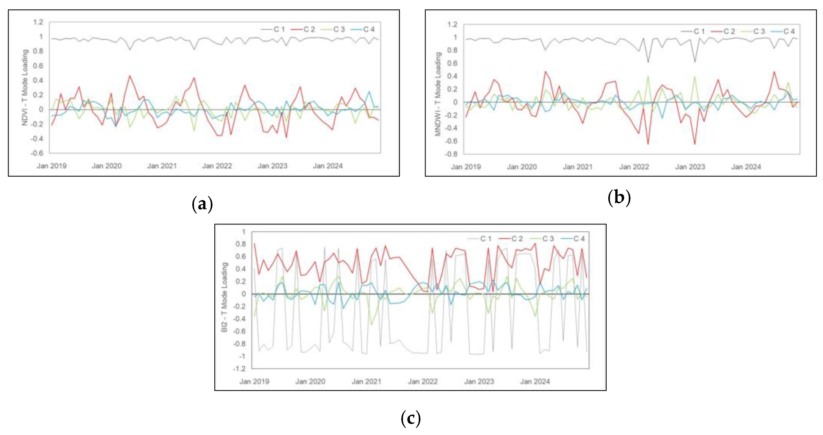
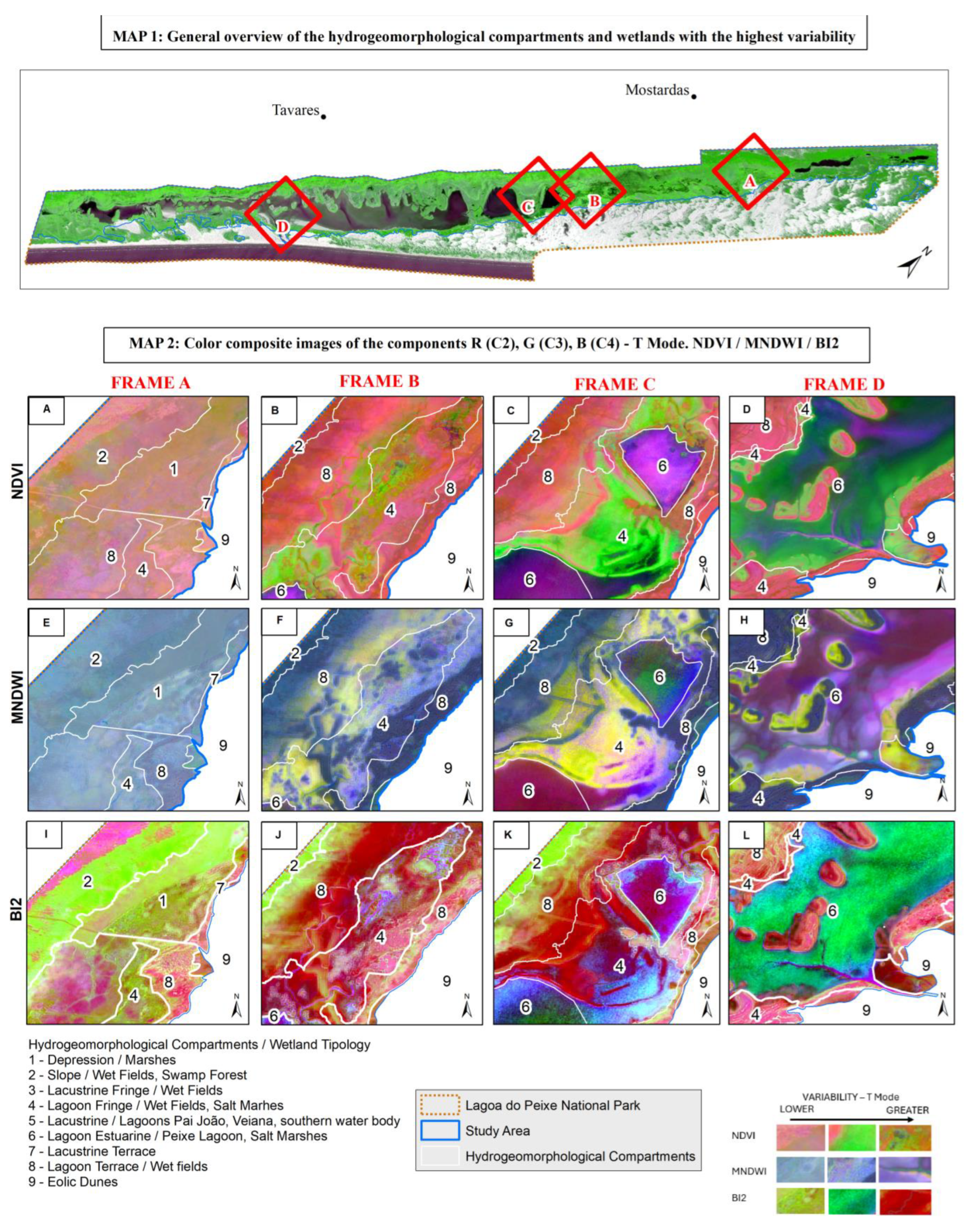
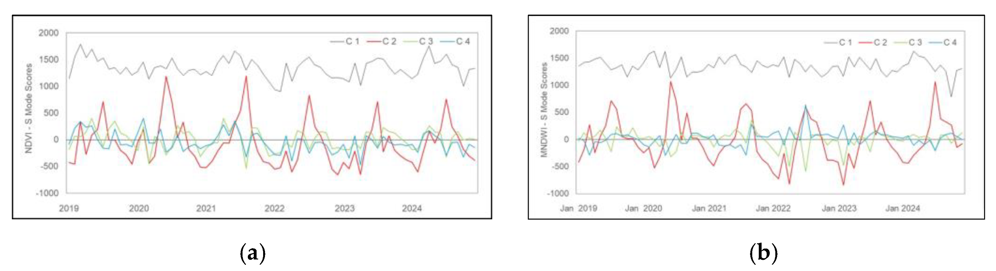
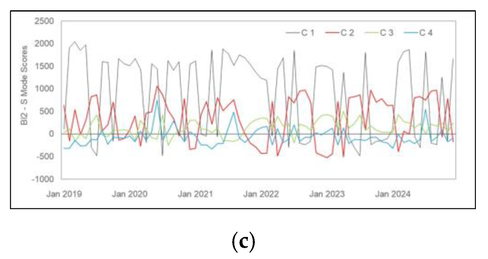
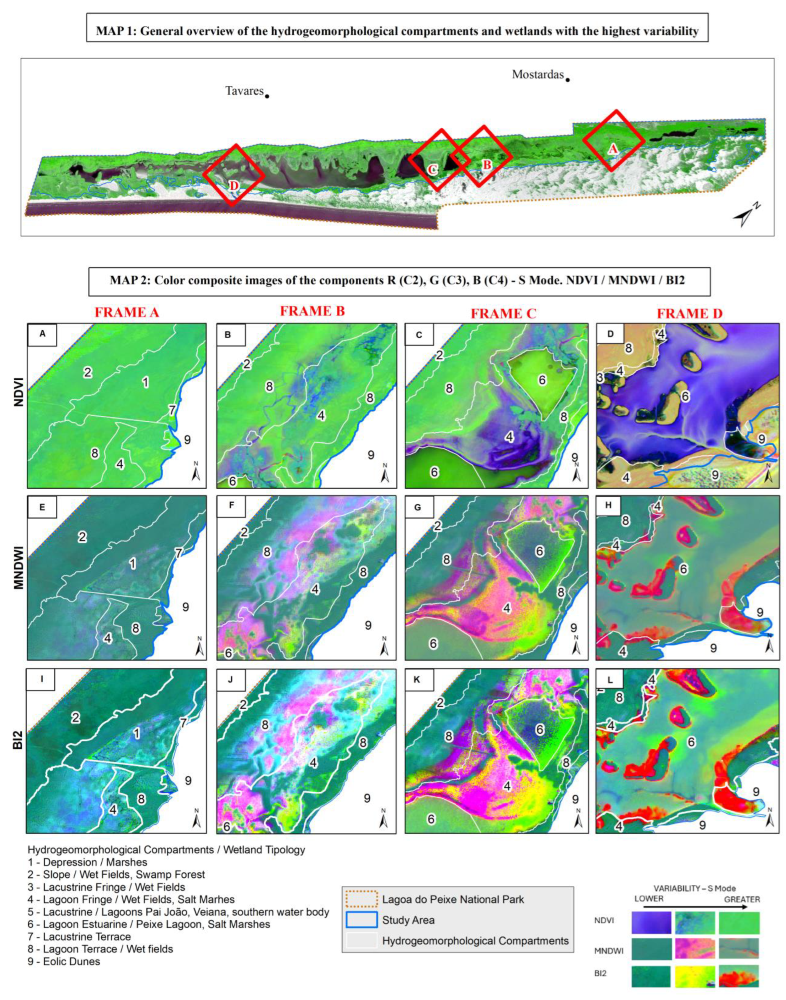
3.1. Temporal and Spatial Variability

The PCA results in T-mode highlight spatial patterns of hydrogeomorphological attributes of coastal wetlands recurring over time. The percentage of variance and eigenvalues (Figure 4) show that the first component (C1) is dominant across all indices, contributing 91.79%, 89.25%, and 62.56% of the variation in NDVI, MNDWI, and BI2, respectively, with high loading values (Figure 5). NDVI and MNDWI exhibit a variance structure concentrated in C1, while BI2 shows a broader distribution with C2, and the loading profile is distributed between C1 and C2 (Figure 5), indicating a temporal dynamics with greater variability.
The loading profiles (Figure 5a–c), obtained from the T-mode analysis, show variations across the historical time series (2019–2024) and highlight distinct behaviors of vegetation cover (NDVI), hydrological regime (MNDWI), and soil characteristics (BI2). NDVI’s Component 2 (C2) stands out with positive peaks during winter (June to August) and negative peaks during summer (December to March). Components 3 (C3) and 4 (C4) display smaller amplitudes, with loading values ranging between −0.2 and 0.2.
The loading profile of MNDWI (Figure 5b) highlights hydrological variations. Although C2 represents less than 10% of the variance, it registers significant oscillations between −0.65 (February 2023) and 0.47 (June 2020). Positive peaks predominate in winter and spring (June to September), while negative peaks occur in summer and autumn. C3 and C4 exhibit more discrete variations, indicating intermediate hydrological patterns in areas with lower flooding frequency, with a water balance regulated by processes such as infiltration, evapotranspiration, and subsurface storage.
The loading profile of BI2 (Figure 5c) highlights patterns in the interaction between soil reflectance, moisture, land cover, and the hydrogeomorphological dynamics of the Coastal wetland. In T-mode, C1 records negative values for most of the time series. C2 presents positive loading values ranging from 0.81 (January 2019) to 0.03 (April 2023). Associated with higher positive loadings, C2 is related to areas of exposed soil and lower surface moisture. C3 and C4, with subtler fluctuations, represent intermediate patterns of moisture and soil exposure, associated with compartments with lower seasonal fluctuations. BI2 proves sensitive to soil moisture dynamics and substrate exposure, differentiating areas of exposed soil from areas with greater water variation.
The color composite images of components C2, C3, and C4 (Figure 6) show recurring spatial patterns over time. In NDVI, C2 highlights areas of greater variability in vegetation, with distinct patterns in the wetlands of the Lacustrine Fringe and the Lagoon Fringe, indicating the differentiated response of vegetation to water influence. C3 and C4 emphasize secondary variations associated with seasonal patterns, with a focus on transition areas between wet fields and lacustrine environments.
In MNDWI, C2 shows greater variability in areas of lagoons and marshes, which are wetlands more sensitive to hydrological variations. In BI2, C2 emphasizes regions with higher soil reflectance, while C3 and C4 display hybrid patterns that highlight the complex spectral response of areas susceptible to temporary flooding and seasonal soil exposure.
The results of the PCA in S-mode highlight temporal patterns of the hydrogeomorphological attributes of the Coastal wetland recurring in space. The percentage of variance and eigenvalues show that C1 represents the dominant spatial pattern in all attributes, contributing 84.70%, 84.98%, and 73.41% of the variation in NDVI, MNDWI, and BI2, respectively, with proportionally high scores (Figure 7).
In NDVI and MNDWI, C2, C3, and C4 capture smaller variations. C2 stands out as the second largest variability, especially in BI2 (16.01%), contrasting with vegetation (NDVI 8.34%) and water (MNDWI 7.82%). The high score value of C2 in BI2 (302.584.66) reinforces its relevance in discriminating secondary temporal patterns recurring in space. Components C3 and C4 represent less than 2% variance in all attributes.
The scores (Figure 8) in S-Mode indicate that C1 exhibits a predominant and stable trend throughout the temporal series for the three indices, reflecting the dominant spatial structure and being less susceptible to seasonal variations. C3 and C4 show variations of smaller amplitude compared to C1 and C2. The scores of these secondary components suggest short-term variations in vegetation cover and less intense spectral response in vegetation.
C2 of NDVI (Figure 8a) shows significant oscillations, with notable positive peaks in the winter months (June to August), with the highest recorded value being 1190.41 (August 2021), corresponding to areas of higher vegetative vigor. In autumn and summer, recurrent negative scores indicate that C2 captures disturbances in vegetation that are not apparent in C1. C3 and C4 show less pronounced variations, reflecting short-duration processes and local changes, with opposing fluctuations in the historical series.
The C2 of the MNDWI (Figure 8b) displays score oscillations reflecting the influence of hydrological events such as floods and droughts. The highest C2 scores occur during winter in all years, while the negative peaks appear in summer, in autumn (2020, 2021, and 2022), and in spring (2022).
The BI2 score profile stood out for presenting a distinct pattern, characterized by oscillations in C1, seasonal variations in C2, stability in C3, and negative values in C4, suggesting a differentiated soil dynamic. The C1 of BI2 (Figure 8c) shows positive score values in 60% of the time series, differing from the T-Mode, which showed negative values. Negative peaks occur throughout the year, mainly concentrated in certain months of summer, autumn, and spring. C2 displays less intense oscillations, with a maximum peak of 1063.18 (June 2020) and the lowest recorded value of −522.32 (January 2023). C3 shows loading values close to zero and predominantly positive, while C4 is mostly negative.
The recurrent temporal patterns of hydrogeomorphological attributes of the coastal wetlands, in the false-color composites C2, C3, and C4 in S-Mode (Figure 9), reveal differences between hydrogeomorphological compartments and wetland typologies. In the NDVI, C2 highlights areas of greater contrast corresponding to wet fields and marshes in the Lagoon Terrace and Lagoon Fringe, as well as palustrine vegetation in the Slope compartment—typologies with higher scores throughout the time series.
The MNDWI color composite highlights flooded areas and water bodies within the Estuarine Lagoon and Lacustrine compartments. C2 enhances the contrast between permanently flooded areas and those that are temporarily saturated. C3 and C4 reveal the influence of seasonal processes, such as water expansion and contraction, as well as the effects of suspended material, particularly in Lagoa do Peixe.
BI2, an indicator of soil moisture and exposed soil presence, shows distinct sensitivity to hydrological and geomorphological variations, with contrasts observed in the Lagoon Fringe, Depression, and parts of the Lagoon Terrace and their corresponding wetlands. The C2 of BI2 emphasizes transitions between wetlands and dry areas, capturing fluctuations in water availability. C3 reflects patterns associated with depositional processes related to flood events and water level retraction.

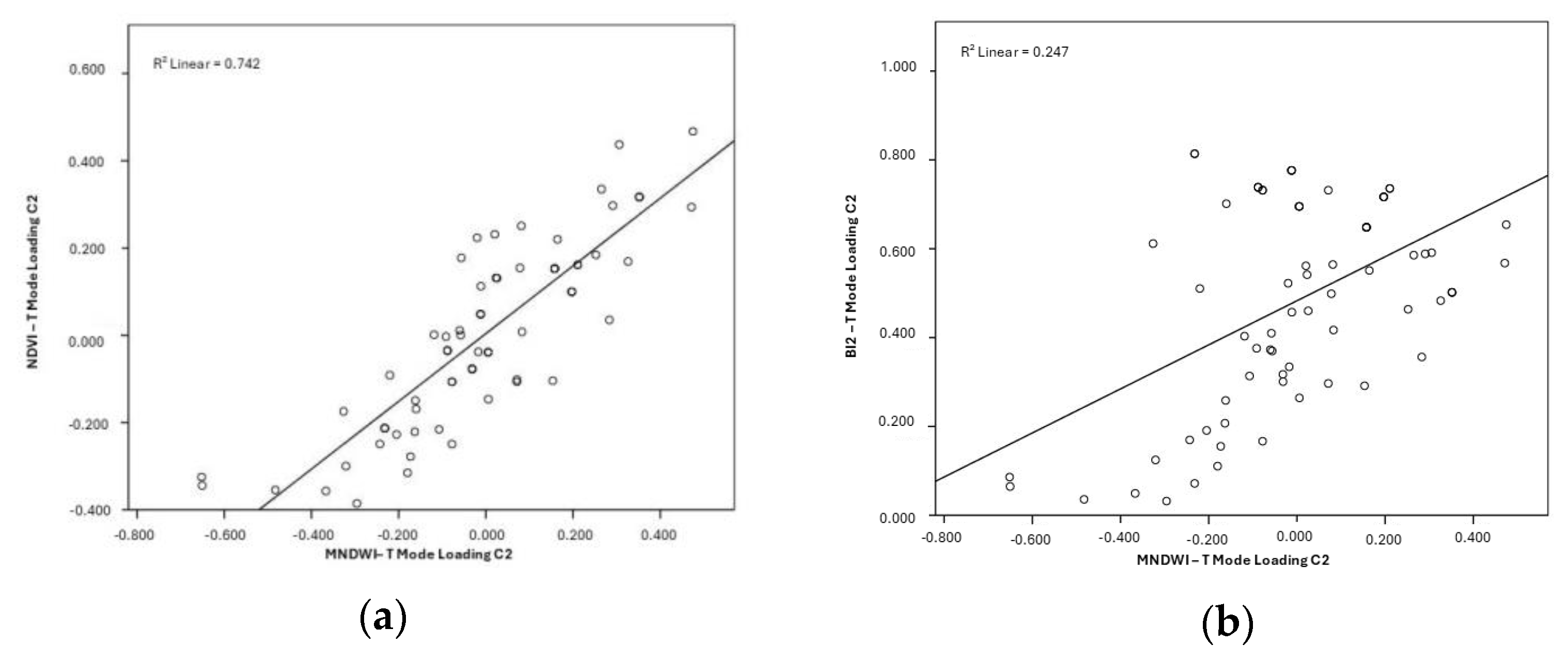
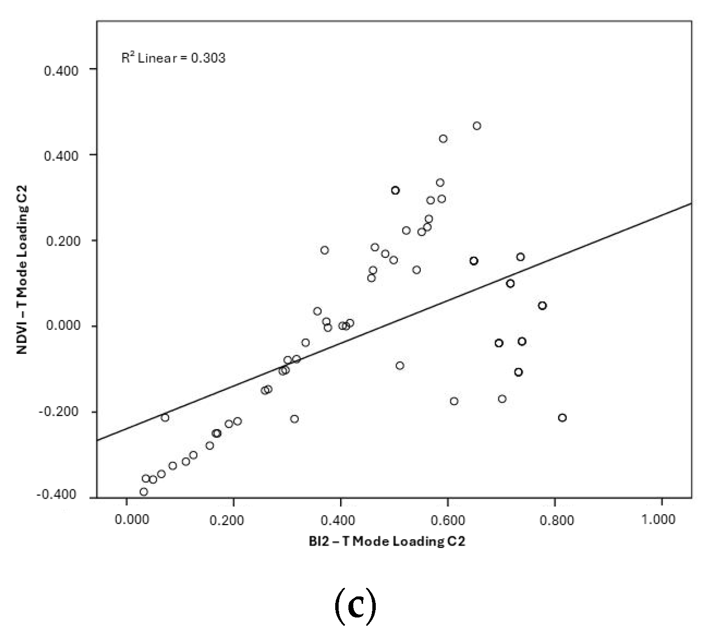
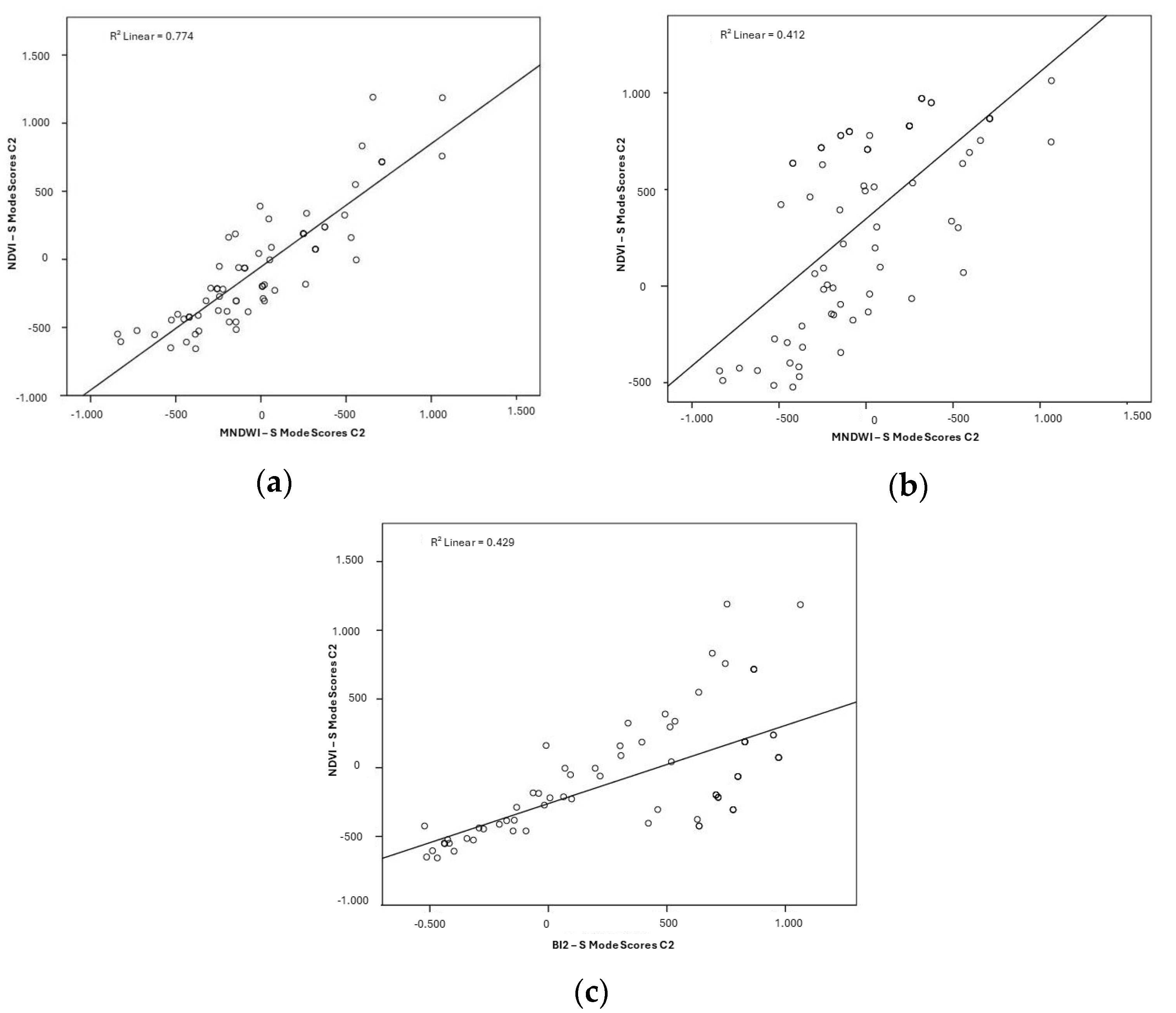
3.2. Relationship Between Hydrogeomorphological Attributes

The Pearson correlation coefficients of the loading values of C2, T-Mode, and the scores, S-Mode, demonstrate statistically significant associations (p < 0.001) between all analyzed combinations (Table 2 and Table 3).
The correlation between NDVI and MNDWI in T-Mode (p = 0.862) and S-Mode (p = 0.880) was strong and positive, indicating an association between vegetation and water surface variability in the compartments. The correlations between NDVI and BI2 (p = 0.550; 0.655) and between MNDWI and BI2 (p = 0.497; 0.642) were moderate and positive, suggesting that soil brightness (BI2) also shares part of the temporal and spatial variability.
The regression lines displayed positive linear trends between the analyzed variables (Figure 10 and Figure 11). Figure 10a shows that 74.2% of the NDVI variability can be explained by MNDWI variations in T-Mode, and 77.4% in S-Mode (Figure 10a). In Figure 10b, in the regression between BI2 and MNDWI, only 24.7% of the BI2 variability is explained by MNDWI changes in T-Mode, and 41.2% in S-Mode (Figure 11b). Between NDVI and BI2 (Figure 10c), 30.3% of the temporal variability of NDVI can be explained by the corresponding variations of BI2 in T-Mode, and 42.9% in S-Mode (Figure 11c).

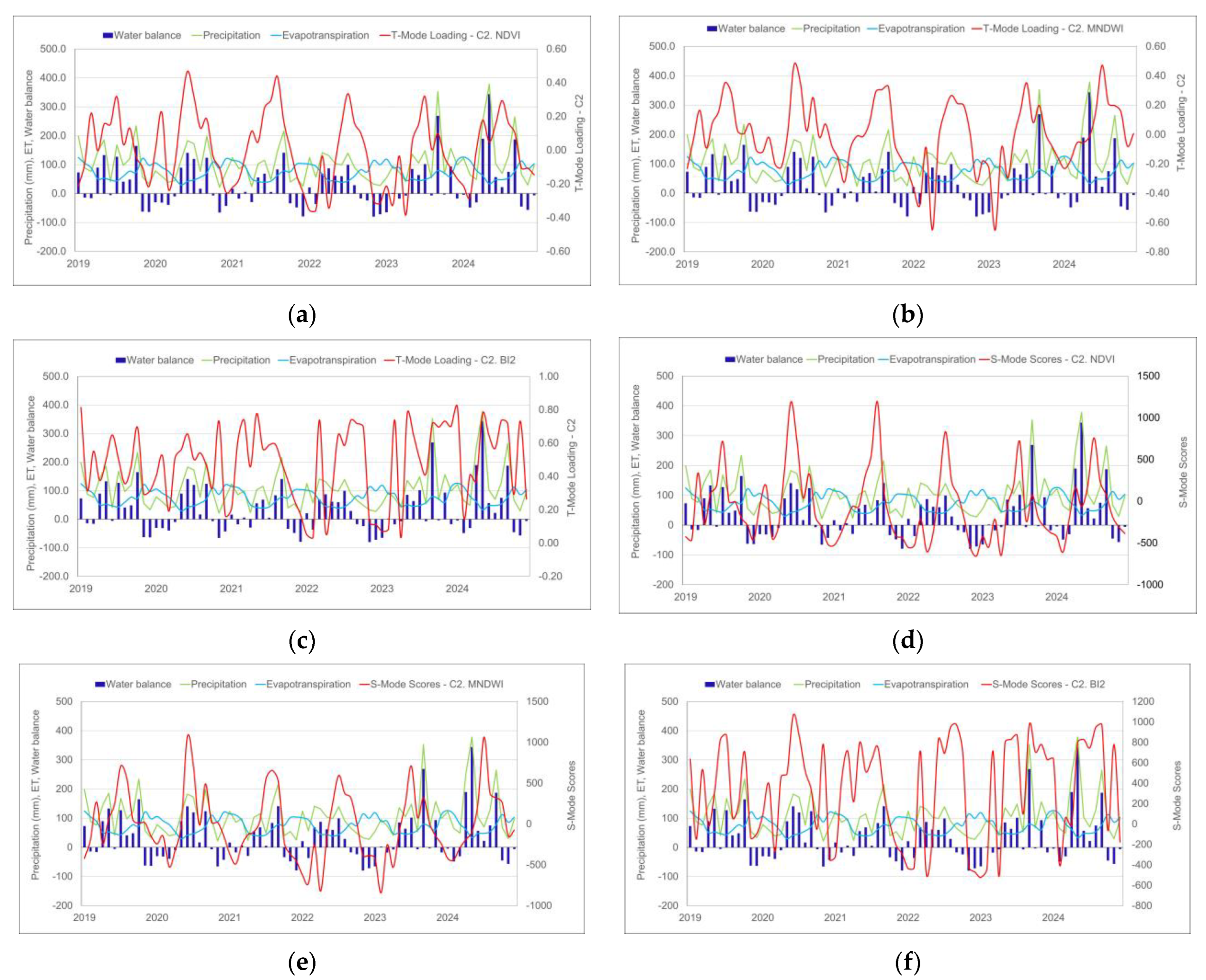
3.3. Hydrogeomorphological Attributes and Water Balance

In the time series (2019–2024), precipitation and evapotranspiration exhibited distinct seasonal patterns (Figure 12a,f), influenced by an extended La Niña period (2020–2023), characterized by water deficit. While precipitation showed greater variations associated with the influence of La Niña and El Niño, evapotranspiration remained relatively stable, with moderate fluctuations. An inverse relationship is observed, with stabilization or reduction of evapotranspiration during periods of higher precipitation, and reduction or constancy during periods of lower precipitation. This dynamic reflects the influence of the water balance in regulating water fluxes in the analyzed system.
The positive and negative peaks of the loading weights (T-Mode) and the scores of C2 (S-Mode) for each attribute follow the variations in the hydrological regime (Figure 12a,f). The highest values occur during periods of higher precipitation and positive water balance, while negative values are related to phases of water deficit. It is noteworthy that the oscillatory behavior of C2 of BI2 (Figure 12c,f) differs from the others, showing a delay in response to the water balance. C2 appears to directly reflect water variations, suggesting a dynamic interaction between vegetation, water availability, and soil structural conditions.

4. Discussion

The characterization of the temporal and spatial variability of hydrogeomorphological attributes (vegetation, water, and soils) in the wetlands of the PNLP allowed the identification of persistent patterns over time, distinguishing them spatially, as well as seasonal or episodic fluctuations. Understanding spatial and temporal behavior is essential for comprehending the hydrogeomorphological dynamics and for guiding conservation strategies aimed at maintaining the environmental health of these systems. The wetlands of the park occupy interdune areas between Barrier III and IV [17,41]. This compartment is characterized by low altimetric variation [22] and is exposed, along with the wetlands, to coastal dynamics, extreme climatic events [44], and anthropogenic impacts.
In this configuration, variability is predominantly determined by biophysical factors. Thus, the method adopted in this analysis was aimed at characterizing and understanding the mechanisms that regulate this variability.
Our study employed multitemporal decomposition in both T-mode (temporal) and S-mode (spatial), combined with the use of spectral indices. In component formation, the T-mode PCA prioritized components that stood out over time, while the S-mode PCA emphasized spatially dominant patterns. These two approaches provided complementary information on the temporal and spatial variability present in the series [67]. Radiometric indices of vegetation, water, and soil are predictive variables that help explain the association among these attributes and the variability of coastal wetlands [68]. Compared to the study conducted in the Pantanal [31], the use of PCA in both T- and S-modes, applied to vegetation radiometric indices, proved effective in investigating the temporal and spatial variability of wetlands.

4.1. Temporal and Spatial Variability

In both T-mode and S-mode, vegetation, water, and soil in the PNLP wetlands exhibited positive linear associations, with high and moderate correlation values. The evidence of temporal variability (T-mode) across space is linked to hydrological events such as floods (El Niño) and droughts (La Niña), which directly affect the vigor and distribution of vegetation cover.
In S-mode, differences between hydrogeomorphological compartments and wetland typologies were identified, with notable contrasts observed among sectors of the Lagoon Terrace, the Lagoon Fringe, and the marsh vegetation areas (located in the Slope compartment).
The interaction between patterns of hydrological variability and the spectral response of vegetation reinforces the importance of spectral indices in monitoring the PNLP wetlands. Seasonal fluctuations in water levels alter vegetation reflectance due to the physiological adjustment of species to water availability [24,69]. The spatial heterogeneity observed in S-Mode suggests that factors such as soil texture, drainage, and hydrological regime influence not only vegetation distribution but also its spectral response over time, directly affecting the ecological stability of these ecosystems [17,25].
Furthermore, the relationship between extreme events, such as El Niño and La Niña, and variability in vegetation cover highlights the sensitivity of wetlands to global climate variations. In similar contexts, research has shown that periods of drought and prolonged flooding are key drivers of hydrogeomorphological variability in wetlands [31,34].

4.2. Hydrogeomorphological Interactions

The strong linear association observed between NDVI and MNDWI reinforces the functional interdependence between vegetation and the presence of surface water in the Lagoa do Peixe National Park wetlands. This pattern highlights that variations in moisture levels directly affect the vigor and distribution of vegetation cover, both temporally and spatially.
On the other hand, the moderate correlations involving BI2 suggest that, although soil brightness is related to hydroecological processes, its behavior is influenced by other environmental factors beyond water availability or vegetation dynamics. The lower predictive capacity of the regressions involving BI2 indicates a more complex and heterogeneous soil response to hydrological processes.
In the interdune area of the study area, corresponding to Lagoon Terraces 1 and 2, hydromorphic sandy-clayey soils predominate [17]. Under natural conditions, hydromorphic soils remain saturated with water, either continuously or during specific periods of the year. These soils have limited drainage, with characteristics resulting from the influence of excessive moisture—either permanent or temporary—caused by the proximity of the water table to the surface during certain times of the year [70].
The relationship between the water balance, loading values, and the scores of hydrogeomorphological attributes revealed well-defined seasonal patterns between precipitation and evapotranspiration, modulated by climatic events associated with the prolonged La Niña period (2020–2022). In contrast, the year 2019, under El Niño influence, was marked by regular rainfall, which contributed to the stability of evapotranspiration observed during the following dry period.
Evapotranspiration in wetlands can remain stable even during periods of water deficit due to a combination of ecohydrological factors, physiological adaptations of vegetation, groundwater storage, or soil moisture [71,72]. Coastal dynamics elements, such as winds and tides, also modulate evapotranspiration behavior, as observed in the coastal wetlands of Chongming Island, China [73], where coastal wind and tidal dynamics introduced complex patterns into evapotranspiration behavior.
The oscillation of loading values (T-mode) and scores (S-mode) found in our study is consistent with research that highlights the direct influence of water availability on wetland dynamics [18,31,46,74,75,76,77,78], and the modulation of hydrogeomorphological processes [35,79,80,81,82,83].
In our study area, this oscillation is clearly expressed in the hydrogeomorphological compartments of Lagoon Terraces 1 and 2, where the interaction between seasonal hydrological dynamics and flat geomorphology intensifies the response of hydrogeomorphological attributes. In the images in color composite (Figure 6 and Figure 9), these evidences reveal spatial and temporal variations associated with hydric dynamics and sedimentary patterns. Characterized by hydromorphic soils and low slope, the Lagoon Terraces show high sensitivity to fluctuations in the water table and to flood pulses, which explains the high loading values of Component 2 (C2) in T-mode, associated with extreme events, as well as the contrasting S-mode scores that distinguish permanently flooded areas from temporarily flooded ones.
This spatial compartmentalization highlights the role of geological characteristics in modulating wetland resilience, with the Lagoon Terraces acting as critical transition zones between lacustrine and palustrine environments. Small hydrological variations in these systems result in significant impacts on vegetation and soil exposure, as indicated by BI2 loadings and scores.
The differentiated response of BI2, in mode T and mode S, suggests the existence of resilience mechanisms or a delay in vegetation response. These mechanisms may be associated with factors such as root system depth, soil water storage capacity, or physiological adaptations [71,72,81]. The spectral behavior of sandy and fine-textured soils, as found in the study area, is another factor that explains this temporal and spatial variability. Sandy soils and those with finer texture have a greater capacity to retain moisture during precipitation events, increasing the absorption of radiant energy and reducing surface reflectance. This pattern is particularly evident in sandy soils with sparse vegetation cover, as occurs in the Laguna Terraces 1 and 2 of the PNLP.
Furthermore, the influence of the soil’s structural conditions can explain variations in the temporal response. Soil texture and porosity affect water retention and redistribution during extreme precipitation events [31,83,84]; this condition of higher soil moisture can modify the vegetation’s response.

5. Conclusions

Given the lack of studies on the Coastal Wetlands system of the PNLP, the characterization of the temporal and spatial variability of hydrogeomorphological attributes (vegetation, water, and soil) has advanced the understanding of the dynamics of the ecosystems in this globally important Ramsar site.
The methodological approach, based on multitemporal analysis of spectral indices (NDVI, MNDWI, and BI2) and Principal Component Analysis (PCA) decomposition in T (temporal) and S (spatial) modes, showed satisfactory results in identifying recurrent patterns and seasonal fluctuations, highlighting contrasts among the hydrogeomorphological compartments. Furthermore, it proved to be a useful tool by revealing previously unknown variabilities of the Coastal Wetlands in the Park. This information is relevant in complex ecosystems where in situ data are scarce and accessibility is limited.
The main contribution of the T-mode analysis was to emphasize that temporal variability responds to climatic extremes, with implications for the conservation of these ecosystems, while in the spatial (S) mode, it is modulated by geomorphology.
The results showed that vegetation (NDVI) and water (MNDWI) present a strong positive correlation, reinforcing the functional interdependence between these attributes. Vegetation cover dynamics respond directly to water variations, with peaks of vegetative vigor associated with periods of higher precipitation and favorable water balance. On the other hand, the soil response (BI2) exhibited greater complexity, indicating influence not only from moisture but also from factors such as texture, surface exposure, and depositional processes. This heterogeneity highlights the importance of integrated analyses to understand the resilience of these ecosystems facing climatic extremes.
The influence of El Niño and La Niña events stood out in modulating hydrogeo-morphological variability, with water deficit periods (La Niña) accentuating temporal and spatial contrasts. Nevertheless, evapotranspiration remained relatively stable, suggesting adaptive vegetation mechanisms and soil water retention. This behavior reinforces the self-regulating capacity of wetlands, although more intense climate changes may challenge their long-term resilience.
From a spatial perspective, the study concludes that the Lagoon Fringe, Lagoon Terrace, and Slope areas showed the greatest variations, reflecting geomorphological differences and hydrological connectivity. These sectors are particularly sensitive to changes in precipitation regimes and extreme coastal events, requiring attention in conservation strategies.

Implications for Conservation and Future Research

The findings of this study highlight the need for the following:
  • Continuous monitoring of coastal wetlands, integrating remote sensing and hydrological data to anticipate responses to climate change;
  • Differentiated protection by compartment, considering the higher sensitivity of areas such as the Lagoon Fringe to hydrological variations;
  • Investigation of subsurface processes, such as water storage and exchanges with the water table, to better understand soil and vegetation resilience.
In summary, the identified variability reflects the complexity and interdependence of hydrogeomorphological attributes in the Lagoa do Peixe National Park, reinforcing its role as a dynamic and sensitive ecosystem. The approach employed can be adapted to other Ramsar sites, contributing to the sustainable management of coastal wetlands facing increasing climatic and anthropogenic pressures.

Author Contributions

C.C.K.: conception, research, methodology, mapping, validation, data preparation, investigation, analysis, and writing of the article; L.A.G.: supervision, research, validation, review, analysis, and writing of the article; H.H.: review, supervision in the TerrSet Libera GIS software; T.F.B.: review, analysis, and writing of the article; C.S.C.: review. All authors have read and agreed to the published version of the manuscript.

Funding

Research funded by the Coordination for the Improvement of Higher Education Personnel (CAPES) through doctoral scholarships, process numbers 88887.645451/2021-00, 88887.488339/2020-00, and 88887.801261/2023-00; CNPq PQ scholarship—process number 301822/2022-0; Foundation for Research Support of the State of Rio Grande do Sul (FAPERGS)—Gaúcho Researcher Program, FAPERGS Public Notice 07/2021.

Institutional Review Board Statement

Not applicable.

Informed Consent Statement

Not applicable.

Data Availability Statement

All data generated or analyzed during this study are included in this published article. More detailed data can be provided upon request to the corresponding author.

Acknowledgments

To the Postgraduate Program in Remote Sensing of the State Center for Research in Remote Sensing and Meteorology/UFRGS; to CAPES and FAPERGS for their financial support. To ICMBio for the authorization for activities for scientific purposes.

Conflicts of Interest

The authors declare no conflicts of interest.

References

  1. Mitsch, W.J.; Bernal, B.; Nahlik, A.M.; Mander, Ü.; Zhang, L.; Anderson, C.J.; Jørgensen, S.E.; Brix, H. Wetlands, Carbon, and Climate Change. Landsc. Ecol. 2013, 28, 583–597. [Google Scholar] [CrossRef]
  2. Simioni, J.P.D. Métodos de Classificação de Imagens de Satélite Para Delineamento de Banhados. Tese de Doutorado, Programa de Pós-Graduação em Sensoriamento Remoto, Universidade Federal do Rio Grande do Sul: Porto Alegre. 2021. Available online: https://lume.ufrgs.br/bitstream/handle/10183/222604/001127156.pdf?sequence=1&isAllowed=y (accessed on 5 January 2025).
  3. Aitali, R.; Snoussi, M.; Kolker, A.S.; Oujidi, B.; Mhammdi, N. Effects of Land Use/Land Cover Changes on Carbon Storage in North African Coastal Wetlands. J. Mar. Sci. Eng. 2022, 10, 364. [Google Scholar] [CrossRef]
  4. Erwin, K.L. Wetlands and Global Climate Change: The Role of Wetland Restoration in a Changing World. Wetl. Ecol Manag. 2009, 17, 71–84. [Google Scholar] [CrossRef]
  5. Ilyas, S.; Xu, X.; Jia, G.; Zhang, A. Interannual Variability of Global Wetlands in Response to El Niño Southern Oscillations (ENSO) and Land-Use. Front. Earth Sci. 2019, 7, 289. [Google Scholar] [CrossRef]
  6. Zhang, Z.; Jiang, W.; Peng, K.; Wu, Z.; Ling, Z.; Li, Z. Assessment of the Impact of Wetland Changes on Carbon Storage in Coastal Urban Agglomerations from 1990 to 2035 in Support of SDG15.1. Sci. Total Environ. 2023, 877, 162824. [Google Scholar] [CrossRef]
  7. Saunois, M.; Jackson, R.B.; Bousquet, P.; Poulter, B.; Canadell, J.G. The Growing Role of Methane in Anthropogenic Climate Change. Environ. Res. Lett. 2016, 11, 120207. [Google Scholar] [CrossRef]
  8. IPBE. The IPBES Regional Assessment Report on Biodiversity and Ecosystem Services for the Americas; Zenodo: Geneva, Switzerland, 2018. [Google Scholar]
  9. Kuenzer, C.; Bluemel, A.; Gebhardt, S.; Quoc, T.V.; Dech, S. Remote Sensing of Mangrove Ecosystems: A Review. Remote Sens. 2011, 3, 878–928. [Google Scholar] [CrossRef]
  10. Mcleod, E.; Chmura, G.L.; Bouillon, S.; Salm, R.; Björk, M.; Duarte, C.M.; Lovelock, C.E.; Schlesinger, W.H.; Silliman, B.R. A Blueprint for Blue Carbon: Toward an Improved Understanding of the Role of Vegetated Coastal Habitats in Sequestering CO2. Front. Ecol. Environ. 2011, 9, 552–560. [Google Scholar] [CrossRef]
  11. Kirwan, M.L.; Megonigal, J.P. Tidal Wetland Stability in the Face of Human Impacts and Sea-Level Rise. Nature 2013, 504, 53–60. [Google Scholar] [CrossRef]
  12. Fluet-Chouinard, E.; Stocker, B.D.; Zhang, Z.; Malhotra, A.; Melton, J.R.; Poulter, B.; Kaplan, J.O.; Goldewijk, K.K.; Siebert, S.; Minayeva, T.; et al. Extensive Global Wetland Loss over the Past Three Centuries. Nature 2023, 614, 281–286. [Google Scholar] [CrossRef]
  13. Xi, Y.; Peng, S.; Ciais, P.; Chen, Y. Future impacts of climate change on inland Ramsar wetlands. Nat. Clim. Change 2021, 11, 45–51. [Google Scholar] [CrossRef]
  14. Hu, S.; Niu, Z.; Chen, Y. Global Wetland Datasets: A Review. Wetlands 2017, 37, 807–817. [Google Scholar] [CrossRef]
  15. Yu, H.; Li, S.; Liang, Z.; Xu, S.; Yang, X.; Li, X. Multi-Source Remote Sensing Data for Wetland Information Extraction: A Case Study of the Nanweng River National Wetland Reserve. Sensors 2024, 24, 6664. [Google Scholar] [CrossRef]
  16. Doughty, C.L.; Ambrose, R.F.; Okin, G.S.; Cavanaugh, K.C. Characterizing Spatial Variability in Coastal Wetland Biomass across Multiple Scales Using UAV and Satellite Imagery. Remote Sens. Ecol. Conserv. 2021, 7, 411–429. [Google Scholar] [CrossRef]
  17. Korb, C.C.; Guasselli, L.A.; Belloli, T.F.; Cunha, C.S.; Bauer, A.L.; dos Santos Brückmann, C. Hydrogeomorphological compartmentalization in coastal wetlands—Lagoa do Peixe National Park, Brazil. Rev. Bras. Geomorfol. 2024, 25, 1–30. [Google Scholar] [CrossRef]
  18. Brinson, M.M. A Hydrogeomorphic Classification for Wetlands; U.S. Army Corps of Engineers: Washington, DC, USA, 1993; Volume 1. [Google Scholar]
  19. Simioni, J.P.D.; Guasselli, L.A.; Etchelar, C.B. Connectivity among Wetlands of EPA of Banhado Grande, RS. RBRH 2017, 22, e15. [Google Scholar] [CrossRef]
  20. Harrison, I.; Abell, R.; Darwall, W.; Thieme, M.L.; Thickner, D.; Timboe, I. The Freshwater Biodiversity Crisis. Science 2018, 362, 1369. [Google Scholar]
  21. Li, Z.; Sun, W.; Chen, H.; Xue, B.; Yu, J.; Tian, Z. Interannual and Seasonal Variations of Hydrological Connectivity in a Large Shallow Wetland of North China Estimated from Landsat 8 Images. Remote Sens. 2021, 13, 1214. [Google Scholar] [CrossRef]
  22. Tagliani, C.R.; Hartmann, C.; Calliari, L.J.; Griep, G.H. Geologia e Geomorfologia da Porção Sul do Parque Nacional da Lagoa do Peixe, RS, Brasil. In Congresso Brasileiro de Geologia, 37; Anais: São Paulo, Brazil, 1992; pp. 292–294. Available online: https://www.sbgeo.org.br/home/pages/44 (accessed on 20 February 2025).
  23. Li, L.; Chen, Y.; Xu, T.; Liu, R.; Shi, K.; Huang, C. Super-Resolution Mapping of Wetland Inundation from Remote Sensing Imagery Based on Integration of Back-Propagation Neural Network and Genetic Algorithm. Remote Sens. Environ. 2015, 164, 142–154. [Google Scholar] [CrossRef]
  24. Rapinel, S.; Mony, C.; Lecoq, L.; Clément, B.; Thomas, A.; Hubert-Moy, L. Evaluation of Sentinel-2 Time-Series for Mapping Floodplain Grassland Plant Communities. Remote Sens. Environ. 2019, 223, 115–129. [Google Scholar] [CrossRef]
  25. Kandus, P.; Minotti, P.G.; Morandeira, N.S.; Grimson, R.; González Trilla, G.; González, E.B.; San Martín, L.; Gayol, M.P. Remote Sensing of Wetlands in South America: Status and Challenges. Int. J. Remote Sens. 2018, 39, 993–1016. [Google Scholar] [CrossRef]
  26. Simioni, J.P.D.; Guasselli, L.A. Dual-Season Comparison of OBIA and Pixel-Based Approaches for Coastal Wetland Classification. RBRH 2024, 29, e5. [Google Scholar] [CrossRef]
  27. Lu, D.; Zheng, Y.; Liu, X.; Chang, J. Changes in Wetland Landscape and Inundation Patterns in the Middle and Lower Reaches of the Yangtze River Basin from 1990 to 2020. Ecol. Indic. 2024, 161, 111992. [Google Scholar] [CrossRef]
  28. Pronk, M.; Hooijer, A.; Eilander, D.; Haag, A.; de Jong, T.; Vousdoukas, M.; Vernimmen, R.; Ledoux, H.; Eleveld, M. DeltaDTM: A Global Coastal Digital Terrain Model. Sci. Data 2024, 11, 273. [Google Scholar] [CrossRef]
  29. Eastman, J.R. TerrSet Libera GIS. Eospatial Monitoring and Modeling System; Tutorial; Version 2024; Clark University: Worcester, MA, USA, 2024. [Google Scholar]
  30. Neeti, N.; Ronald Eastman, J. Novel Approaches in Extended Principal Component Analysis to Compare Spatio-Temporal Patterns among Multiple Image Time Series. Remote Sens. Environ. 2014, 148, 84–96. [Google Scholar] [CrossRef]
  31. de Almeida, T.I.R.; Penatti, N.C.; Ferreira, L.G.; Arantes, A.E.; do Amaral, C.H. Principal Component Analysis Applied to a Time Series of MODIS Images: The Spatio-Temporal Variability of the Pantanal Wetland, Brazil. Wetl. Ecol. Manag. 2015, 23, 737–748. [Google Scholar] [CrossRef]
  32. Pereira, L.E.; Noveli, R.A.P.; Filho, A.C.P. Uso de Análise de Componentes Principais (PCA) para Caracterização das Sub-Regiões do Megaleque do Taquari—Pantanal. Rev. GeoPantanal. 2023, 18, 114–126. [Google Scholar] [CrossRef]
  33. Munyati, C. Use of Principal Component Analysis (PCA) of Remote Sensing Images in Wetland Change Detection on the Kafue Flats, Zambia. Geocarto Int. 2004, 19, 11–22. [Google Scholar] [CrossRef]
  34. Mattson, M.; Sousa, D.; Quandt, A.; Ganster, P.; Biggs, T. Mapping Multi-Decadal Wetland Loss: Comparative Analysis of Linear and Nonlinear Spatiotemporal Characterization. Remote Sens. Environ. 2024, 302, 113969. [Google Scholar] [CrossRef]
  35. Berlanga-Robles, C.A. Trends in Mangrove Canopy and Cover in the Teacapan-Agua Brava Lagoon System (Marismas Nacionales) in Mexico: An Approach Using Open-Access Geospatial Data. Wetlands 2024, 45, 1. [Google Scholar] [CrossRef]
  36. Nepita-Villanueva, M.R.; Berlanga-Robles, C.A.; Ruiz-Luna, A.; Morales Barcenas, J.H. Spatio-Temporal Mangrove Canopy Variation (2001–2016) Assessed Using the MODIS Enhanced Vegetation Index (EVI). J. Coast Conserv. 2019, 23, 589–597. [Google Scholar] [CrossRef]
  37. Zhang, X.; Wang, G.; Xue, B.; Zhang, M.; Tan, Z. Dynamic Landscapes and the Driving Forces in the Yellow River Delta Wetland Region in the Past Four Decades. Sci. Total Environ. 2021, 787, 147644. [Google Scholar] [CrossRef]
  38. Rolon, A.S. Diversidade de Macrófitas Aquáticas Em Áreas Úmidas Do Parque Nacional Da Lagoa Do Peixe, Rio Grande Do Sul. Ph.D. Thesis, Universidade Federal de São Carlos, Sao Carlos, Brazil, 2011. Available online: https://repositorio.ufscar.br/handle/20.500.14289/1740 (accessed on 27 December 2024).
  39. Costa, J.C.; Pereira, G.; Siqueira, M.E.; Cardozo, F.d.S.; da Silva, V.V. Validação dos Dados de Precipitação Estimados pelo CHIRPS para o Brasil. Rev. Bras. Climatol. 2019, 24, 228–243. [Google Scholar] [CrossRef]
  40. Garcia, A.; Winemiller, K.; Hoeinghaus, D.; Claudino, M.; Bastos, R.; Correa, F.; Huckembeck, S.; Vieira, J.; Loebmann, D.; Abreu, P.; et al. Hydrologic Pulsing Promotes Spatial Connectivity and Food Web Subsidies in a Subtropical Coastal Ecosystem. Mar. Ecol. Prog. Ser. 2017, 567, 17–28. [Google Scholar] [CrossRef]
  41. Arejano, T.B. Geologia e Evolução Holocênica do Sistema Lagunar da Lagoa do Peixe, Litoral Médio do Rio Grande Do Sul, Brasil. Ph.D. Thesis, Programa de Pós-Graduação em Geociências, Universidade Federal do Rio Grande do Sul, Porto Alegre, Brazil, 2006. Available online: https://lume.ufrgs.br/handle/10183/8527 (accessed on 26 December 2024).
  42. Sbruzzi, J.B. Análise da Dinâmica da Embocadura da Lagoa do Peixe—RS Utilizando Dados de Sensoriamento Remoto Orbital. Master’s Thesis, Programa de Pós-Graduação em Sensoriamento Remoto, Universidade Federal do Rio Grande do Sul, Porto Alegre, Brazil, 2015. Available online: https://lume.ufrgs.br/bitstream/handle/10183/130851/000979924.pdf?sequence=1&isAllowed=y (accessed on 21 December 2024).
  43. Schossler, V. Morfodinâmica da Embocadura da Lagoa do Peixe e da Linha de Praia Adjacente. Master’s Thesis, Programa de Pós-Graduação em Geociências, Universidade Federal do Rio Grande do Sul, Porto Alegre, Brazil, 2011. Available online: https://lume.ufrgs.br/bitstream/handle/10183/32663/000786858.pdf?sequence=1&isAllowed=y (accessed on 27 December 2024).
  44. Schossler, V. Influência das Mudanças Climáticas em Geoindicadores na Costa Sul do Brasil. Ph.D. Thesis, Programa de Pós-Graduação em Geociências, Universidade Federal do Rio Grande do Sul, Porto Alegre, 2016. Available online: https://lume.ufrgs.br/bitstream/handle/10183/149450/001006590.pdf?sequence=1&isAllowed=y (accessed on 28 December 2024).
  45. Manzolli, R.P.; Portz, L.C.; Fontán-Bouzas, A.; Bitencourt, V.J.B.; Alcántara-Carrió, J. Contribution of Reverse Dune Migration to Stabilization of a Transgressive Coastal Dune Field at Lagoa do Peixe National Park Dune Field (South of Brazil). Remote Sens. 2023, 15, 3470. [Google Scholar] [CrossRef]
  46. Korb, C.C.; Guasselli, L.A.; Belloli, T.F.; Cunha, C.S. Dinâmica espaço-temporal de pulsos de inundações nas Áreas Úmidas do Parque Nacional da Lagoa do Peixe, sul do Brasil. Investig. Geogr. Una Mirada Desde El Sur 2023, 1, 32–47. [Google Scholar] [CrossRef]
  47. Junk, W.J. Definição, Delineamento e Classificação Brasileira das Áreas Úmidas. In Inventário das Áreas Úmidas Brasileiras: Distribuição, Ecologia, Manejo, Ameaças e Lacunas de Conhecimento; Carlini & Caniato Editorial: Cuiabá, Brazil, 2024; pp. 29–42. ISBN 978-85-8009-353-7. Available online: https://inau.org.br/site/images/e-book/c_c_inventario_das_areas_umidas_brasileiras_inau_e-book.pdf (accessed on 20 December 2024).
  48. Villwock, J.A.; Tomazelli, L.J.; Loss, E.L.; Dehnhardt, E.A.; Bachi, F.A.; Dehnhardt, B.A. Quaternary of South America and Antarctic Peninsula. Geol. Rio Gd. Do Sul Coast. Prov. 1986, 4, 79–97. [Google Scholar]
  49. Tomazelli, L.J.; Villwock, J.A. O Cenozóico do Rio Grande do Sul: Geologia da Planície Costeira. In Geologia do Rio Grande do Sul; Holz, F., DeRos, L.F., Eds.; UFRGS: Porto Alegre, Brazil, 2000; p. 444. [Google Scholar]
  50. Schäffer, A.; Lanzer, R.; Scur, L. Atlas Socioambiental Dos Municípios de Cidreira, Balneário Pinhal, Palmares Do Sul; Editora da Universidade de Caxias do Sul: Caxias do Sul, Brazil, 2013; Available online: https://www.ucs.br/educs/livro/atlas-socioambiental-dos-municipios-de-cideira-balneario-pinhal-e-palmares-do-sul-projeto-lagoas-costeiras-ii/ (accessed on 26 December 2024).
  51. Ramos, R.A.; Pasqualeto, A.I.; Balbueno, R.A.; Das Neves, D.D.; De Quadros, E.L.L. Mapeamento e Diagnóstico de Áreas Úmidas No Rio Grande Do Sul, Com o Uso de Ferramentas de Geoprocessamento. In Proceedings of the Anais, Porto Alegre, Brazil, 2014; pp. 17–21. [Google Scholar]
  52. Belloli, T.F.; Guasselli, L.A.; Cunha, C.S.; Korb, C.C. Mudanças e Transição da Cobertura e Uso da Terra nas Áreas Úmidas da Região Geomorfológica Planície Costeira—RS. Geo UERJ 2024, 1, 1–24. [Google Scholar] [CrossRef]
  53. Moraes, V.L. Uso do Solo e Conservação Ambiental no Parque Nacional da Lagoa do Peixe e Entorno (RS). Master’s Thesis, Programa de Pós-Graduação em Geografia, Universidade Federal do Rio Grande do Sul, Porto Alegre, Brazil, 2009. Available online: https://lume.ufrgs.br/bitstream/handle/10183/23706/000738097.pdf?sequence=1&isAllowed=y (accessed on 19 December 2024).
  54. Portz, L.C.; Guasselli, L.A.; Corrêa, I.C.S. Variação Espacial e Temporal de NDVI na Lagoa do Peixe, RS. Rev. Bras. Geogr. Física 2011, 5, 897–908. [Google Scholar]
  55. IBGE. Banco de Dados e Informações Ambientais (BDIA). Mapeamento de Recursos Naturais (MRN), Escala 1:250 000. 2023. Available online: https://www.ibge.gov.br/pt/inicio.html (accessed on 1 December 2024).
  56. ICMBio. Limites Oficiais de Unidades de Conservação Federais. 2024. Available online: https://www.gov.br/icmbio/pt-br/assuntos/dados_geoespaciais/mapa-tematico-e-dados-geoestatisticos-das-unidades-de-conservacao-federais. (accessed on 1 December 2024).
  57. Streck, E.V.; Kämpf, N.; Dalmolin, R.S.D.; Klamt, E.; Nascimento, P.C.; Scheneider, P.; Giasson, E.; Pinto, L.F.S. Solos Do Rio Grande Do Sul, 2nd ed.; Emater-Ascar: Porto Alegre, Brazil, 2008. [Google Scholar]
  58. Signori, L.M. Mapeamento espaço temporal da exótica invasora Pinus spp. na área norte do Parque Nacional da Lagoa do Peixe. Master’s Thesis, Programa de Pós-Graduação em Sensoriamento Remoto, Universidade Federal do Rio Grande do Sul, Porto Alegre, Brazil, 2018. Available online: https://lume.ufrgs.br/bitstream/handle/10183/179643/001069723.pdf?sequence=1&isAllowed=y (accessed on 1 December 2024).
  59. Portz, L.; Manzolli, R.P.; Alcántara-Carrió, J.; Rockett, G.C.; Barboza, E.G. Degradation of a Transgressive Coastal Dunefield by Pines Plantation and Strategies for Recuperation (Lagoa Do Peixe National Park, Southern Brazil). Estuar. Coast. Shelf Sci. 2021, 259, 107483. [Google Scholar] [CrossRef]
  60. Reboita, M.S.; Ambrizzi, T.; da Rocha, R.P. Relationship between the Southern Annular Mode and Southern Hemisphere Atmospheric Systems Relação Entre o Modo Anular Sul e os Sistemas Atmosféricos no Hemisfério Sul. Rev. Bras. Meteorol. 2009, 24, 48–55. [Google Scholar] [CrossRef]
  61. Fontana, D.C.; Berlato, M.A. Influência do El Niño Oscilação Sul sobre a precipitação do Estado do Rio Grande do Sul. Rev. Bras. Agrometeorol. 1997, 5, 127–132. Available online: https://revistas.ufpr.br/revistaabclima/article/view/25408 (accessed on 2 January 2025).
  62. Britto, F.P.; Barletta, R.; Mendonça, M. Variabilidade Espacial e Temporal da Precipitação Pluvial no Rio Grande Do Sul: Influência do fenômeno El Niño Oscilação Sul. Rev. Bras. Climatol. 2008, 3, 37–48. [Google Scholar] [CrossRef]
  63. Rodrigues, B.D. Comportamento Dos Sistemas Frontais No Estado Do Rio Grande Do Sul Durante Os Episódios ENOS. Master’s Thesis, Programa de Pós-Graduação em Sensoriamento Remoto, Universidade Federal do Rio Grande do Sul, Porto Alegre, Brazil, 2015. Available online: https://lume.ufrgs.br/bitstream/handle/10183/139305/000989919.pdf?sequence=1&isAllowed=y (accessed on 2 January 2025).
  64. Rouse, J.W.; Haas, R.H.; Schell, J.A.; Deering, D.W. Monitoring Vegetation Systems in the Great Plains with ERTS (Earth Resources Technology Satellite); Greenbelt: Austin, TX, USA, 1973; pp. 309–317. [Google Scholar]
  65. Xu, H. Modification of Normalised Difference Water Index (NDWI) to Enhance Open Water Features in Remotely Sensed Imagery. Int. J. Remote Sens. 2006, 27, 3025–3033. [Google Scholar] [CrossRef]
  66. Escadafal, R. Remote Sensing of Arid Soil Surface Color with Landsat Thematic Mapper. Adv. Space Res. 1989, 9, 159–163. [Google Scholar] [CrossRef]
  67. Machado-Machado, E.A.; Neeti, N.; Eastman, J.R.; Chen, H. Implications of Space-Time Orientation for Principal Components Analysis of Earth Observation Image Time Series. Earth Sci. Inf. 2011, 4, 117–124. [Google Scholar] [CrossRef]
  68. Ramsar Convention Secretariat. Wetland Inventory: A Ramsar Framework for Wetland Inventory and Ecological Character Description, 4th ed.; Ramsar Convention Secretariat: Gland, Switzerland, 2010; Volume 15. [Google Scholar]
  69. Jensen, J.R. Sensoriamenro Remoto Do Ambiente: Uma Perspectiva Em Recursos Terrestre; Parêntese: Sao Jose dos Campos, Brazil, 2009. [Google Scholar]
  70. Empresa Brasileira de Pesquisa Agropecuária. Sistema Brasileiro de Classificação de Solos, 2nd ed.; Embrapa Solos: Rio de Janeiro, Brazil, 2006. [Google Scholar]
  71. Giardina, F.; Gentine, P.; Konings, A.G.; Seneviratne, S.I.; Stocker, B.D. Diagnosing Evapotranspiration Responses to Water Deficit across Biomes Using Deep Learning. New Phytol. 2023, 240, 968–983. [Google Scholar] [CrossRef] [PubMed]
  72. Stocker, B.D.; Tumber-Dávila, S.J.; Konings, A.G.; Anderson, M.C.; Hain, C.; Jackson, R.B. Global Patterns of Water Storage in the Rooting Zones of Vegetation. Nat. Geosci. 2023, 16, 250–256. [Google Scholar] [CrossRef]
  73. Huang, Y.; Guo, H.; Chen, X.; Chen, Z.; van der Tol, C.; Zhou, Y.; Tang, J. Meteorological Controls on Evapotranspiration over a Coastal Salt Marsh Ecosystem under Tidal Influence. Agric. For. Meteorol. 2019, 279, 107755. [Google Scholar] [CrossRef]
  74. Dronova, I.; Gong, P.; Wang, L.; Zhong, L. Mapping Dynamic Cover Types in a Large Seasonally Flooded Wetland Using Extended Principal Component Analysis and Object-Based Classification. Remote Sens. Environ. 2015, 158, 193–206. [Google Scholar] [CrossRef]
  75. Rioja-Nieto, R.; Barrera-Falcón, E.; Torres-Irineo, E.; Mendoza-González, G.; Cuervo-Robayo, A.P. Environmental Drivers of Decadal Change of a Mangrove Forest in the North Coast of the Yucatan Peninsula, Mexico. J. Coast Conserv. 2017, 21, 167–175. [Google Scholar] [CrossRef]
  76. Penatti, N.C.; de Almeida, T.I.R.; Ferreira, L.G.; Arantes, A.E.; Coe, M.T. Satellite-Based Hydrological Dynamics of the World’s Largest Continuous Wetland. Remote Sens. Environ. 2015, 170, 1–13. [Google Scholar] [CrossRef]
  77. Junk, W.J.; Bayley, P.B.; Sparks, R.E. Flood Pulse Concept in River—Floodplain-Systems. Can. J. Fish. Aquat. Sci. 1989, 106, 110–127. [Google Scholar]
  78. Wei, S.; Han, G.; Chu, X.; Sun, B.; Song, W.; He, W.; Wang, X.; Li, P.; Yu, D. Prolonged Impacts of Extreme Precipitation Events Weakened Annual Ecosystem CO2 Sink Strength in a Coastal Wetland. Agric. For. Meteorol. 2021, 310, 108655. [Google Scholar] [CrossRef]
  79. Ablat, X.; Liu, G.; Liu, Q.; Huang, C. Using MODIS-NDVI Time Series to Quantify the Vegetation Responses to River Hydro-Geomorphology in the Wandering River Floodplain in an Arid Region. Water 2021, 13, 2269. [Google Scholar] [CrossRef]
  80. Daly, E.; Porporato, A. Impact of Hydroclimatic Fluctuations on the Soil Water Balance. Water Resour. Res. 2006, 42, W06401. [Google Scholar] [CrossRef]
  81. Singh, M.; Sinha, R. Hydrogeomorphic Indicators of Wetland Health Inferred from Multi-Temporal Remote Sensing Data for a New Ramsar Site (Kaabar Tal), India. Ecol. Indic. 2021, 127, 107739. [Google Scholar] [CrossRef]
  82. Lee, O.; Kim, H.S.; Kim, S. Hydrological Simple Water Balance Modeling for Increasing Geographically Isolated Doline Wetland Functions and Its Application to Climate Change. Ecol. Eng. 2020, 149, 105812. [Google Scholar] [CrossRef]
  83. Penatti, N.C.; de Almeida, T.I.R. Subdvision of Pantanal Quaternary Wetlands: MODIS NDVI Time Series in the Indirect Detection of Sediments Granulometry. Int. Arch. Photogramm. Remote Sens. Spat. Inf. Sci. 2012, 39, 311–316. [Google Scholar] [CrossRef]
  84. Narváez-Salcedo, S.; Hoyos, N.; Aldana-Domínguez, J. Spatial and Temporal Trend of EVI in Mangrove Forests of Coastal Lagoons in the Colombian Caribbean; Universidad del Norte: Barranquilla, Colombia, 2022. [Google Scholar]
Figure 1. (A) Study area location; (A, B, C, D) Highlighted hydrogeomorphological compartments. (B) Hydrogeomorphological compartments. Sources: colored composition R3G8B4 Sentinel 2; [17,55,56].
Coasts 05 00023 g001
Figure 2. Coastal wetlands of the study area. (A) Peixe Lagoon, salt marshes; (B) wet fields swamp forest; (C) marshes; (D) wet fields. Photos: by the authors.
Coasts 05 00023 g002
Figure 3. Methodological framework of the study. Sources: Geomorphological compartments [41]; Hydrogeomorphological compartments [17]; Mapping WET [51].
Coasts 05 00023 g003
Figure 4. Percentage of variance and eigenvalues associated with each Principal Component and hydrogeomorphological attribute, T-Mode.
Coasts 05 00023 g004
Figure 5. Loading profiles by hydrogeomorphological attribute, T-Mode. The black, red, green, and blue lines correspond to the temporal variation (C1, C2, C3, and C4), respectively; and loading profiles (a) of NDVI, (b) MNDWI, and (c) BI2.
Coasts 05 00023 g005
Figure 6. MAP 1: Location of hydrogeomorphological compartments with the highest variability. Sentinel-2 image in false-color composition (R3G8B4); A, B, C, D represent highlighted hydrogeomorphological compartments. MAP 2: T-Mode analysis of wetland typologies within the hydrogeomorphological compartments. Color composite images of components R (C2), G (C3), and B (C4), for the variables NDVI (AD), MNDWI (EH) and BI2 (IL).
Coasts 05 00023 g006
Figure 7. Percentage of variance and eigenvalues associated with each Principal Component and hydrogeomorphological attribute, S-Mode.
Coasts 05 00023 g007
Figure 8. Score profiles, S-Mode by hydrogeomorphological attribute in the 2019–2024 time series. The black, red, green, and blue lines represent C1, C2, C3, and C4, respectively, and loading profiles of (a) NDVI, (b) MNDWI, and (c) BI2.
Coasts 05 00023 g008aCoasts 05 00023 g008b
Figure 9. MAP 1: Location of hydrogeomorphological compartments with the highest variability. Sentinel-2 image in false-color composition (R3G8B4); A, B, C, D represent highlighted hydrogeomorphological compartments. MAP 2: S-Mode analysis of wetland typologies within the hydrogeomorphological compartments. Color composite images of components R (C2), G (C3), and B (C4), for the variables NDVI (AD), MNDWI (EH) and BI2 (IL).
Coasts 05 00023 g009
Figure 10. Scatter diagrams of the hydrogeomorphological attributes, C2, T-Mode. (a): NDVI (dependent variable) and MNDWI (predictor variable); (b) BI2 (dependent variable) and MNDWI (predictor variable); (c) NDVI (dependent variable) and BI2 (predictor variable).
Coasts 05 00023 g010aCoasts 05 00023 g010b
Figure 11. Scatter diagrams of the hydrogeomorphological attributes, C2, S-Mode. (a): NDVI (dependent variable) and MNDWI (predictor variable); (b) BI2 (dependent variable) and MNDWI (predictor variable); (c) NDVI (dependent variable) and BI2 (predictor variable).
Coasts 05 00023 g011
Figure 12. Estimated values of precipitation, evapotranspiration, and water balance from 2019 to 2024. Component 2 (C2) loadings and scores by hydrogeomorphological attribute, presented for both T-Mode and S-Mode analyses. NDVI (a,d), MNDWI (b,e), and BI2 (c,f).
Coasts 05 00023 g012
Table 1. Indices espectrais utilizados no estudo.
Hydrogeomorphological Attribute/VariableFormulaReference
Normalized Difference Vegetation Index (NDVI) ( N I R r e d ) ( N I R + r e d ) [64]
Modified Normalized Difference Water Index (MNDWI) ( g r e e n S W I R 1 ) ( g r e e n + S W I R 1 ) [65]
Second Brightness Index (BI2) r e d 2 + g r e e n 2 + N I R 2 3 [66]
Table 2. Pearson Correlation Matrix—C2, T-Mode.
NDVIMNDWIBI2
NDVIPearson Correlation---
p value---
MNDWIPearson Correlation0.862--
p valuep < 0.001--
BI2Pearson Correlation0.5500.497-
p valuep < 0.001p < 0.001-
Table 3. Pearson Correlation Matrix—C2, S-Mode.
NDVIMNDWIBI2
NDVIPearson Correlation---
p value---
MNDWIPearson Correlation0.880--
p valuep < 0.001--
BI2Pearson Correlation0.6550.642-
p valuep < 0.001p < 0.001-
Disclaimer/Publisher’s Note: The statements, opinions and data contained in all publications are solely those of the individual author(s) and contributor(s) and not of MDPI and/or the editor(s). MDPI and/or the editor(s) disclaim responsibility for any injury to people or property resulting from any ideas, methods, instructions or products referred to in the content.

