1. Introduction
In regions like western Norway, western Canada, and Chilean Patagonia, above 45 degrees latitude, characterized by prominent fjord environments, recurrent glaciations during the Pleistocene epoch have resulted in steep slopes, creating conditions favorable for landslide-triggered tsunamis. These mountainous environments are prone to rock falls, slides, and avalanches, which can trigger tsunami waves [
1].
The destructive power of subaerial landslide-triggered tsunamis is evident in a small number of well-documented events. These waves can produce run-up heights exceeding hundreds of meters, significantly higher than those typically generated by earthquakes. For instance, the 1948 Lituya Bay (USA) event witnessed a staggering 524 m run-up, while the 1963 Vajont Valley (Italy) and 1980 Spirit Lake (USA) events saw run-ups of 250 and 260 m, respectively [
1]. Another noteworthy characteristic of landslide-generated tsunamis is their recurrence rate. Ref. [
2] documented historical run-up events in Lituya Bay, including 120 m in 1853–1854, 24 m in 1874, 60 m in 1899, and 150 m in 1936 [
3].
Tsunamigenic geohazards in southern Chile, particularly south of the triple junction, have been poorly studied due to the inaccessibility of the terrain and the scarcity of geophysical data. The Patagonian fjord region, one of the most extensive in the world, has a high potential for generating tsunamis due to earthquakes, landslides, and ice calving. Chile, with over half of the western margin of the South American subduction zone and where Patagonian fjords account for more than 42% of the country’s continental coastline, offers a unique case study.
Despite limited historical and instrumental data in Chile’s southern Liquiñe-Ofqui Fault zone (LOFZ), evidence suggests recurring seismic swarms along the fault (see
Figure 1). Seismic swarms can trigger landslide-generated tsunamis. Historical seismic activity includes a magnitude 7.1 earthquake on 21 November 1927, approximately 100 km north of the Aysén Fjord [
4]. Other notable events are the 21 April 2007, Aysén earthquake [
5], and the 2008 Chaitén eruption [
6]. Between 23 January and mid-June 2007, a local seismic network recorded more than 7200 seismic events [
7]. Then, the Aysén swarms and main earthquake represent a great opportunity to study the seismotectonic structure, due to the low seismic activity of the region, the Chilean Patagonia [
8].
On 21 April 2007, a magnitude 6.2 earthquake struck the Aysén region in southern Chile, triggering massive landslides that caused a devastating tsunami in the Aysén Fjord. This event is significant as it represents the first instrumentally recorded case of a landslide-generated tsunami in Chile.
Tragically, this event resulted in 10 fatalities and the destruction of several salmon farms along the fjord [
9]. Extensive seismic activity induced fear, panic, and other psychological impacts on the populations of Chacabuco Port and Aysén Port, as well as salmon farm workers [
5,
10].
Historically, shallow-water theory has been widely used to model tsunamis, assuming that the tsunami wavelength significantly exceeds the water depth. For these long waves, wave dispersion (ref. [
11] defines it as a phenomenon where different wave components within a wave train propagate at varying speeds due to their differing wavelengths, resulting in energy wave spreading as wave travels) can be neglected as the phase velocity depends solely on water depth. However, landslide-generated waves are often classified as intermediate or deep-water waves. Given their relatively short wavelengths, dispersion becomes a significant factor in their propagation, as the phase velocity is influenced by both water depth and wavelength [
12].
Modeling landslide-generated tsunamis presents a challenge due to the computational cost and the need to accurately represent the nonlinear and dispersive behavior of the generated waves. Given the substantial influence of dispersion on landslide-generated tsunamis, which are characteristically prevalent in intermediate and deep-water wave domains, researchers are compelled to employ higher-order Boussinesq-type wave equations (BWEs) in place of shallow-water equations (SWEs) when developing two-layer models [
13].
Various studies have addressed the modeling of landslide-generated tsunamis in fjords or lakes, each contributing valuable insights. Ref. [
14] demonstrated the effectiveness of Lagrangian nonlinear models in predicting inundation, highlighting the importance of constructive interference in wave amplification. Ref. [
15] developed a tsunami early warning system specifically for the island of Crete (in the Eastern Mediterranean Basin—EMB), based on the assimilation of data from a network of 12 strategically located offshore bottom pressure gauges (OBPGs) around the island. This system utilizes data assimilation to generate accurate forecasts and is applicable to tsunamis generated by both earthquakes and landslides in the Eastern Mediterranean region. Their results demonstrate the capability of OBPG data assimilation to satisfactorily predict the amplitudes and arrival times of tsunamis in the EMB. Ref. [
16] explored the influence of idealized bathymetries using SWASH, developing predictive methods with neural networks and regressions. Ref. [
17] introduced a three-dimensional granular model, validated with Lake Askja data, simulating the complete event chain. Collectively, these studies underscore the need for tailored models and high-quality data to enhance the prediction and understanding of these complex phenomena. Ref. [
18] used the Cornell multi-grid coupled Tsunami model (COMCOT) to simulate the Aysén tsunami of 21 April 2007, incorporating the landslides north of Mentirosa Island and at Punta Cola. Ref. [
18] found that their model reproduced run-up heights well compared to field measurements near the landslide–fjord contact zones. However, the model results diverged from measurements by a factor of 2–3 in areas farther away. This discrepancy can be attributed to several factors, including the use of coarse spatial discretization (50 m × 50 m) in the model setup. However, the most significant factor is the inability of the long wave-based models to properly represent frequency dispersion, a phenomenon characteristic of tsunamis generated by submarine and subaerial landslides.
This study aims to investigate the mechanisms behind the landslide-generated tsunami of 21 April 2007, focusing on the generation, propagation, and run-up phases. To simulate this event, we employ the NHWAVE and FUNWAVE-TVD models to simulate the 2007 Aysén tsunami, focusing on the landslides at Punta Cola and north of Mentirosa Island. Two modeling approaches are employed: a viscous fluid model and a solid (rigid) model. The selection of these landslides, based on their volume and location, and the data availability for the tsunami-triggering landslides, is justified by the arguments presented by [
19], who identify them as the primary generators of the tsunami. Additionally, the availability of detailed data on these landslides allows for the rigorous validation of the numerical models. While other smaller landslides also contributed to the event, the selected ones provide a solid foundation for understanding the generation and propagation mechanisms of the 2007 Aysén tsunami. One of the objectives of this study is also to corroborate whether the parameters reported by various authors (for example, [
5]) are capable of explaining the phenomenon, both in terms of reported run-up heights and inundation zones. Finally, the benchmark for evaluating the behavior of our simulations is the tide gauge located in Chacabuco Port (the only tide gauge that recorded the tsunami).
In
Section 2, we present a brief description of the geological context of the Aysén region, Chile.
Section 3 presents a comprehensive overview of the methodology utilized.
Section 4 presents the results. Discussion is addressed in
Section 5. Finally, the conclusions are presented in
Section 6.
2. Geological and Seismotectonic Context of the Aysén Region, Chile
Chile is one of the most seismically active countries in the world. It experiences major earthquakes, exceeding a magnitude of 8, roughly every ten years. Between 1962 and 1997 alone, over 4000 earthquakes greater than 5 were recorded. Notably, seismic activity is not uniformly distributed throughout the country [
20].
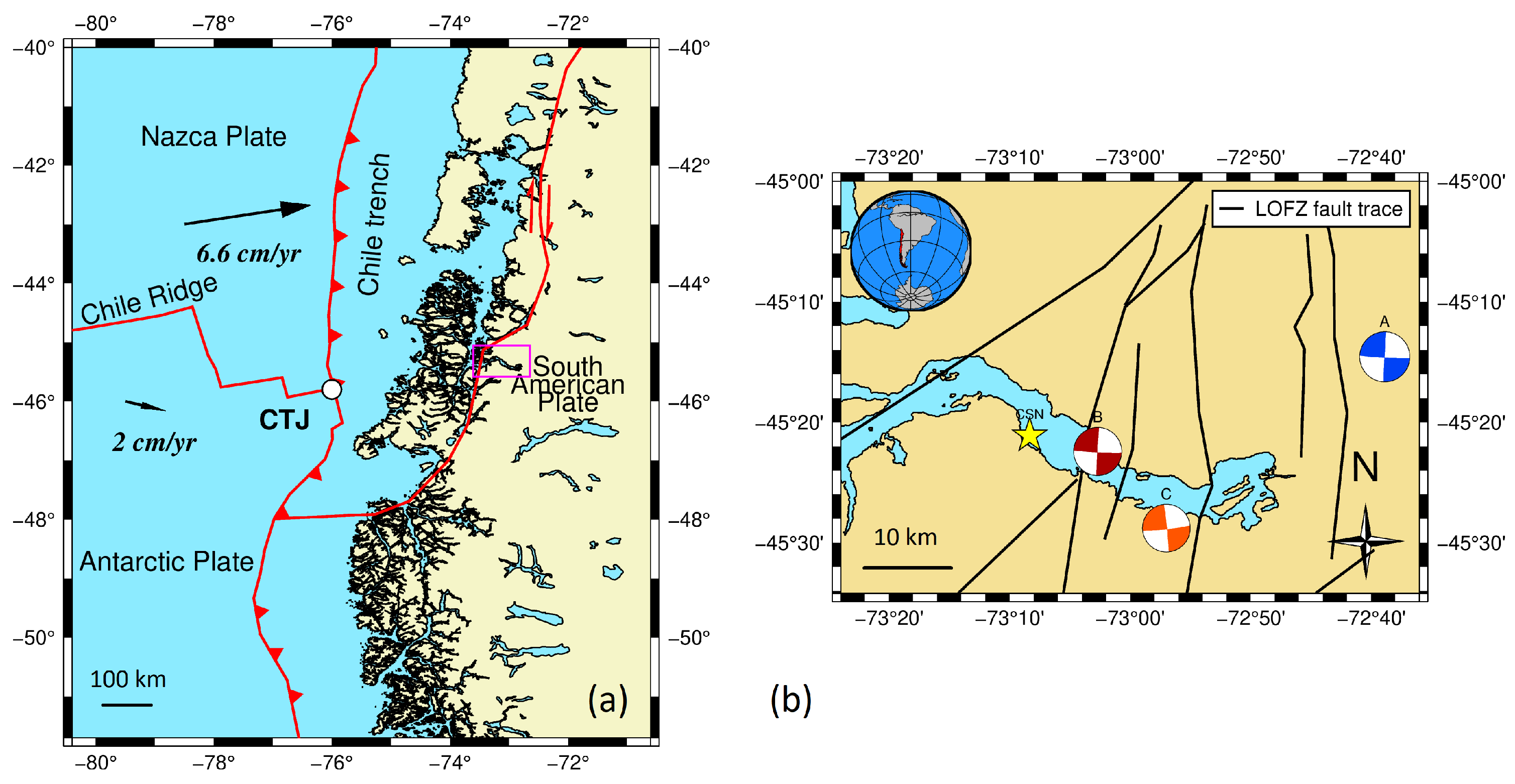
Oceanic and continental tectonic plates move at different speeds. For example, the Nazca plate subducts under the South American plate move at a much faster rate (see
Figure 2a), 6.6 cm/year [
21], compared to the 2 cm/year rate of the Antarctic plate (south of the Taitao Peninsula) [
22]. The angle of convergence between the Nazca and South American plates is about 18° [
7,
21]. The Chilean triple junction (CTJ) region undergoes a complex deformation process characterized by both brittle, seismic events, and ductile, aseismic strain. This duality contributes to significant uncertainties in the region’s tectonic behavior.
The North Patagonian Batholith (NPB) is the dominant geological feature of Chilean Patagonia, and is composed of three belts: the easternmost dominated by mid-Cretaceous monzogranites and granites, the central belt featuring Miocene granodiorite-diorite with minor granites, and the westernmost boasting granodiorites spanning the Jurassic to Cretaceous period. The NPB is accompanied by various formations and units, including the Cretaceous Traiguén Formation (composed of metasedimentary and metavolcanic rocks), a Paleozoic metamorphic basement, and Pleistocene-Holocene volcanic units [
23].
The Aysén Fjord, our area of interest, showcases a more varied geological composition. Here, foliated gabbros, diorites, quartz diorites, granodiorites, and tonalites coexist alongside dike groupings, gneissic bands, and volcanic deposits of the Macá-Cay complex [
19].
2.1. The 2007 Aysén Earthquake
The dominant tectonic feature of the study region is the LOFZ. This fault system is a dextral strike-slip fault system exceeding 1000 km in length and trending NNE (
Figure 2a). Among the master faults there are 4 NE-trending échelon faults consisting of a strike-slip duplex [
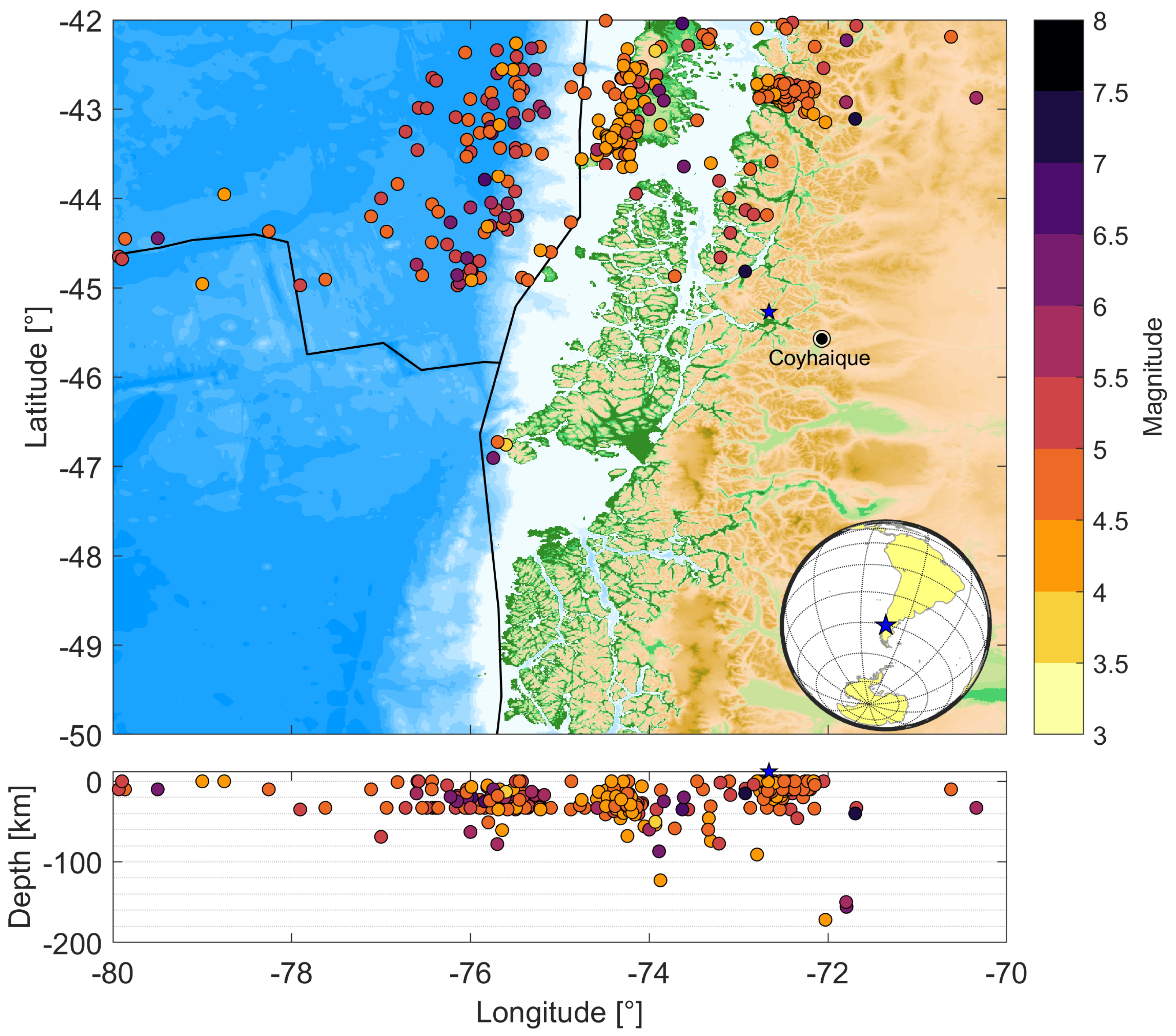
8]. The figure presented below illustrates the seismicity of the Aysén region, representing the location of seismic events using latitude and longitude coordinates, in addition to their depth.
Figure 1 shows global seismicity from 1964 until 2024. The catalog was obtained from the National Seismological Center (CSN, in Spanish), upon request (
www.csn.uchile.cl (accessed on 9 May 2025)). The whole catalog was normalized and equalized to moment magnitude Mw. Seismicity confirms a remarkable drop-off in the seismicity rate from the triple joint (around 45S–46S), which responds to the different tectonic setting due to the velocity convergence of the Nazca plate versus the Antarctic plate. Also, the station coverage in the southern part of Chile and Argentina is low and there are some natural biases in the catalog analysis. In the
Supplementary Materials (S5), a complementary analysis of the seismicity data was conducted to derive a local Gutenberg–Richter law (G–R law).
Figure 1.
Historical seismicity in the studied region. Black lines represent the boundaries of the tectonic plates. Blue star denotes the 2007 Aysen earthquake.
Figure 1.
Historical seismicity in the studied region. Black lines represent the boundaries of the tectonic plates. Blue star denotes the 2007 Aysen earthquake.
Aysén Fjord began experiencing a seismic cluster on 10 January with a minor quake (magnitude less than 3). Aftershocks followed, culminating in a 5.2 magnitude earthquake on 23 January, triggering a surge of over 20 events per hour. The origin, debated as volcanic (see [
24]) or tectonic (see [
25]), was followed by five larger earthquakes exceeding a magnitude of 5 throughout the year, as can be seen in the NEIC catalog [
8].
The mainshock of moment magnitude (M
w) 6.2 occurred at 17:53 local time on 21 April 2007. According to the NEIC-USGS catalog, the focal mechanism of the mainshock indicates dextral strike-slip faulting along a NNE-trending fault of the LOFZ [
8]. Ref. [
7] determined the focal mechanism to have the following failure plane parameters: dip = 84°/354°, strike = 86°/88°, and rake = 2°/176°.
Ref. [
7] relocated the main earthquake epicenter to −45.374° latitude and −73.045° longitude, also adjusting the hypocenter depth to 4 km (previously estimated at 12 km by the GCMT catalog). Subsequently, ref. [
8], using the initial parameters from the USGS catalog, the hypocenter depth was relocated, obtaining a value of 8 km (initially estimated at 36.7 km).
Figure 2.
(
a) Tectonic setting of the Aysén Region, Chile. The magenta rectangle is the zoom of the right panel; (
b) Epicenters of the 21 April 2007 Aysén earthquake in Chilean Patagonia. The blue beach ball (A) represents the NEIC solution, the red beach ball (B) indicates the focal mechanism solution from [
7], the orange beach ball (C) corresponds to the GCMT solution, and the yellow star marks the hypocenter as determined by the CSN. The black solid line marks the trace of the LOFZ.
Due to the limited instrumentation in the study area, the hypocenter’s location is uncertain. In contrast to models that directly couple the seismic fault with tsunami generation, and despite the potential influence of this uncertainty on such models, our study focuses on the hydrodynamic response to the multiple landslides that were the primary cause of the tsunami.
Figure 2b illustrates the Aysén Fjord alongside the focal mechanism of the Mw 6.2 mainshock (red beach ball) determined by [
7], with a hypocentral depth of 4 km. Ref. [
26] provides details on the trace of the Liquiñe-Ofqui Fault zone (LOFZ).
Table 1 summarizes the geographic coordinates of the hypocenter of the mainshock that occurred in Aysén on 21 April 2007. It provides the latitude, longitude, and depth of the earthquake.
The 21 April 2007 earthquake triggered 541 mass wasting events, classified as rock slides/avalanches, rock falls, shallow soil/soil–rock slides, and debris flows, identified through remote sensing analysis and field observations [
19].
2.2. Main Landslides
Two major landslides were reported during the earthquake. One originated on the northern side of the fjord, directly opposite Mentirosa Island (MI), and the other, the Punta Cola landslide (PC), originated in a lateral glacial valley. Both landslides reached the fjord, generating tsunami waves [
18].
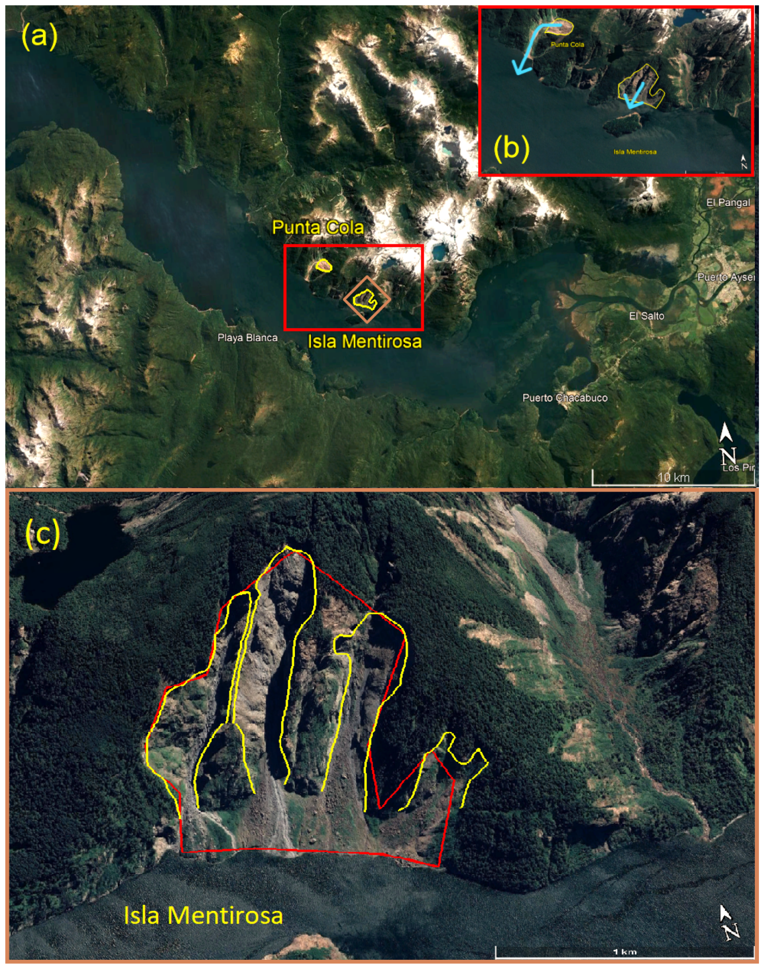
Ref. [
19] classified the Punta Cola landslide as a rockslide and avalanche. The centroid of the main landslide is located at (656844, 4972725) in the WGS84 coordinate system, specifically UTM–18S, at an elevation of 565 m above sea level (see
Figure 3b). The landslide originated from the NPB, with a maximum thickness of 135 m, which fragmented and traveled down the slope, reaching a maximum run-up of 180 m on the opposite bank [
27].
As [
29] describes, the Punta Cola landslide is a complex mass movement of eight individual landslides that contributed to the event. The largest of these was a rock avalanche, accompanied by seven smaller, secondary landslides. Ref. [
19] classified the overall movement as rockslides and avalanches. The landslide traveled a distance of 1.5 km before reaching the fjord and generating tsunami waves.
One of the first investigations into the 2007 Aysén tsunami was conducted by [
30], who classified the landslide on the north side of Mentirosa Island as a rockslide. Ref. [
28] provided a detailed visual description of this landslide, noting it consists of four soil-rock slides (see
Figure 3c). The centroid of the landslide is located at (659097, 4970580) in the WGS84 coordinate system, specifically UTM–18S, at an altitude of 390 m (see
Figure 3b).
Ref. [
31] observed the topographic amplification of seismic waves at the landslide site, as all the individual slides originated near the mountain peak. This suggests that after, the initial movement and fragmentation, each soil-rock slide may have transformed into a rock avalanche or debris flow before reaching the water surface. Additionally, ref. [
28] also noted inverse grading at the base of the largest landslide, where larger boulders accumulated at the top of the debris fan (farthest from the water).
2.3. Landslide Tsunami
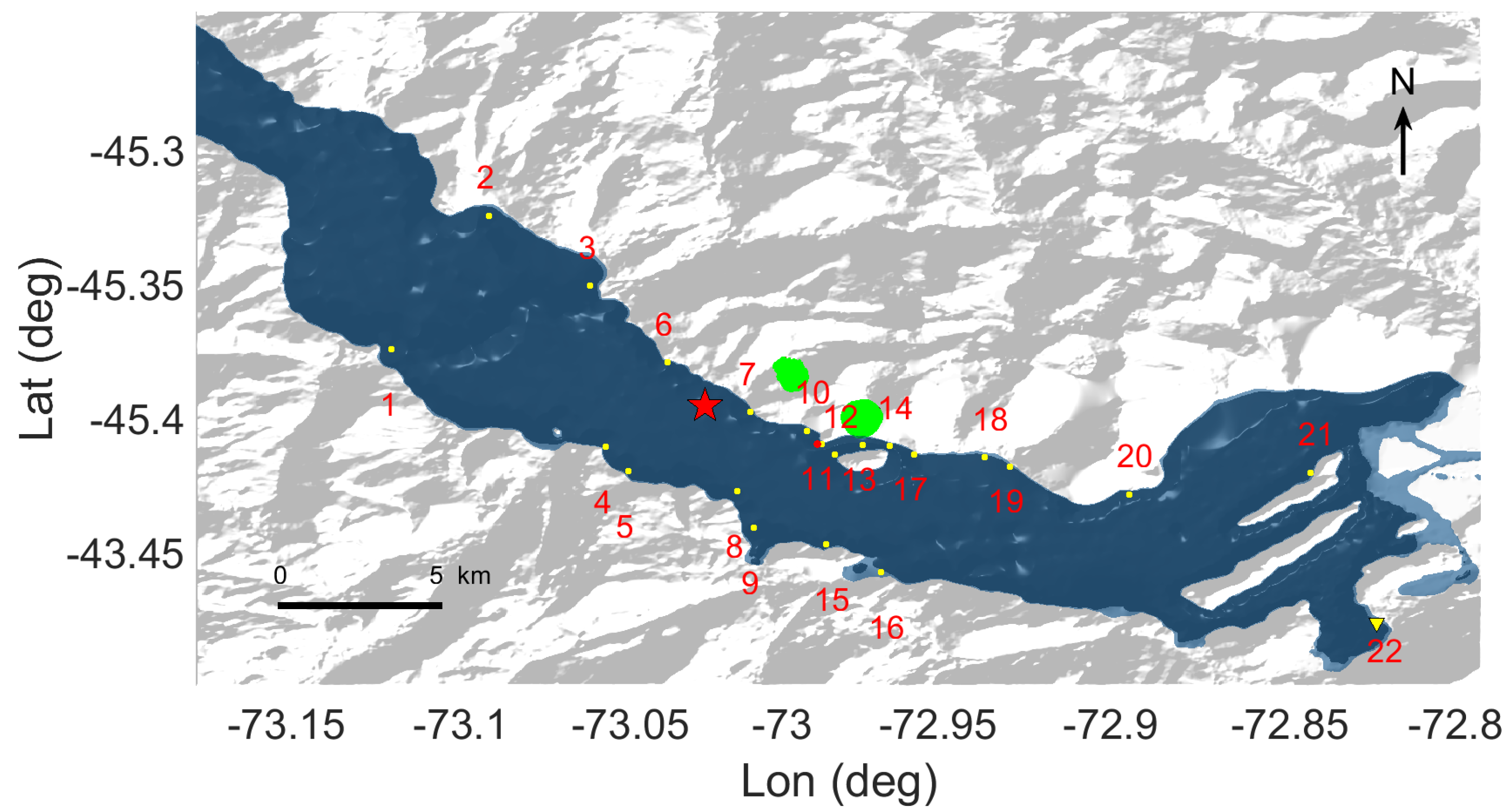
Large volumes of rock and debris entered the Aysén Fjord from landslides north of Mentirosa Island (point 13,
Figure 4), Quebrada Sin Nombre (point 7,
Figure 4), and east of Aguas Calientes (point 8,
Figure 4). According to [
5], the failures occurred almost simultaneously and within less than a minute after the main earthquake. The set of landslides triggered a sequence of tsunami waves within the fjord. The Aysén incident highlighted the substantial influence that subaerial landslides can exert on the fjord [
32].
The landslide generated a series of large waves near Mentirosa Island, with maximum run-up reaching approximately 50 m [
18,
33]. The forceful impact of the displaced water on the northern flank of Mentirosa Island destabilized soil and vegetation, leaving impact marks up to several tens of meters high [
5].
Figure 4 shows the location (yellow points) of run-up heights measured by National Geology and Mining Service (SERNAGEOMIN, in Spanish). However, no tide correction was informed and no specific time and date for the measurement was included in the data [
33]. These points are the places of run-up heights data that we will use to compare with our synthetic data. SERNAGEOMIN measured all data points in
Figure 4, except for the Chacabuco tide gauge (Point 22,
Figure 4).
The sole tide gauge in the Aysén Fjord, situated in Chacabuco Port, is used to validate and constrain the synthetic time series generated by our simulations.
3. Methodology
To understand the generation and propagation mechanisms of the landslide-generated tsunami that occurred in the Aysén Fjord on 21 April 2007, a numerical modeling approach using NHWAVE and FUNWAVE-TVD models has been adopted. This study aims to simulate the PC and MI landslides, in order to assess their contribution to the observed tsunami, considering factors such as arrival time in Chacabuco Port, run-up heights, and inundation zones. To capture the complex dynamics of the Aysén tsunami, we employ the FUNWAVE-TVD and NHWAVE models. FUNWAVE-TVD is a fully nonlinear dispersive Boussinesq long-wave model [
34]. FUNWAVE-TVD was run using the NHWAVE output at
s on a 30 m pixel size grid to prevent computational instabilities. Given its significantly faster computational speed compared to NHWAVE, FUNWAVE-TVD enabled a substantial reduction in computation time when using a larger computational grid. The NHWAVE output at
s, containing the water surface elevation,
x direction velocity, and
y direction velocity, is transferred as the initial condition for the FUNWAVE-TVD simulation. Once this transfer is complete, FUNWAVE-TVD can be run with different input parameters and for a significantly longer duration than NHWAVE. The final step involves the manual coupling of the time series generated by both NHWAVE and FUNWAVE-TVD.
NHWAVE is a publicly available, open source software that solves the incompressible Navier–Stokes equation using a small number of vertical, boundary fitted,
-layers. This allows for a more realistic simulation compared to simpler depth-averaged models, as NHWAVE can incorporate multiple vertical levels [
35]. Both NHWAVE and FUNWAVE-TVD have been validated through scientific publications and are used by various research groups [
34]. NHWAVE’s complete treatment of non-hydrostatic wave dispersion allows for a more accurate representation of frequency dispersion than traditional nonlinear shallow-water equation (NLSWE) models [
36].
Regarding data acquisition, landslide-generated tsunami modeling requires various high-resolution data sources, such as topography and bathymetry, to accurately represent the real-world surface. To describe the source of the tsunami, it requires the geometry, centroid coordinates, rheology, and kinematics of the landslide. It is important to note that the landslides are modeled independently of the earthquake (no earthquake coupling). To model the 2007 Aysén tsunami, we used bathymetry data provided by the Hydrographic and Oceanographic Service of the Chilean Navy (SHOA, in Spanish) and topography data from the USGS EarthExplorer (
https://earthexplorer.usgs.gov/ (accessed on 19 January 2024)). The source bathymetry data exhibit varying point density, while the topography data maintains a consistent resolution of 1 arc second. Using these datasets, we constructed the joint surface representing the intersection of topography and bathymetry, i.e., a digital elevation model (DEM). Note that the discretization of the topography directly determines the grid size of the bathymetric-topographic surface, as reflected in the values of
and
in
Table 2.
3.1. Modeling of the 2007 Aysén Landslide Tsunami
Given the rheological characteristics of the study area, we designed six modeling scenarios to explore the potential impacts of different landslide types on tsunami generation. To address the reported landslide volumes (see
Table 3 and
Table 4), we modeled two distinct rheologies: viscous and solid with Coulomb friction angle. Additionally, we explored an extreme case by assuming landslides with no basal friction. This resulted in a total of six numerical simulations.
These six modeling scenarios, labeled E1–E6, were designed to investigate the influence of landslide rheology on simulation outcomes, with a focus on the geological conditions of the Aysén fjord. Two landslides are modeled as viscous (semi-ellipsoidal shape), while the others have a solid, slab geometry (see
Figure 5). Input data for all landslides are provided in
Table 3 and
Table 4. Both the Mentirosa Island (MI) and Punta Cola (PC) landslides can be simulated with either viscous or solid properties. For the solid case, we consider two scenarios: (1) a Coulomb friction angle (
) based on Aysén fjord rock type, and (2) a no basal friction scenario (
). Landslide dimensions are derived from their volume and plan area. NHWAVE software calculates landslide velocity during simulations, but we use initial velocities from [
5]. In all simulations (E1–E6), both landslides are assumed to initiate simultaneously.
Table 2 shows that the computational domain extends over an area of 41.4 km by 25.2 km, encompassing the study region (see
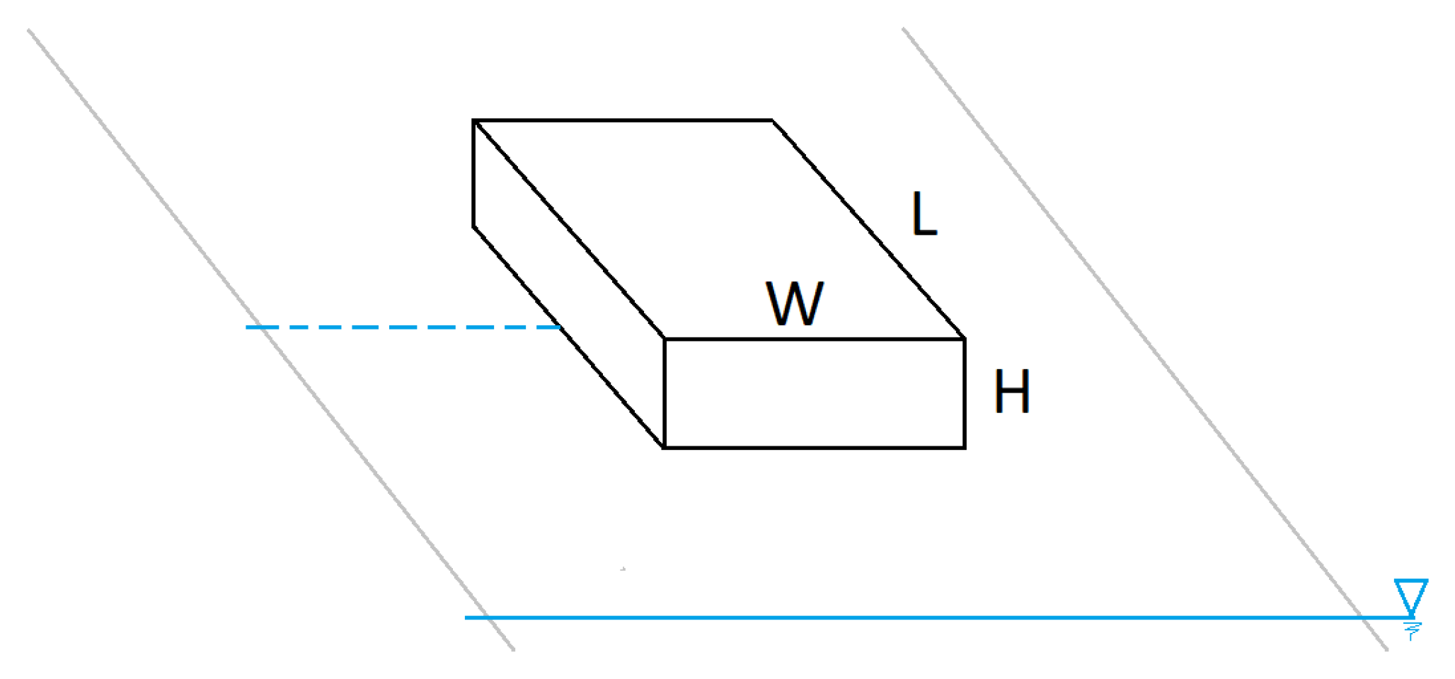
Figure 3). The topographic data employed have a spatial resolution of 30 m, corresponding to the most detailed scale obtainable from public sources. The simulation, with a duration of 1 h, accounts for the stages of generation, propagation, and run-up of tsunami waves. This ensures the analysis of run-up heights, arrival times, and inundation zones. The following figure schematizes the subaerial landslide that will be modeled.
Figure 5 illustrates the shape of the representative landslide to be modeled in the NHWAVE, along with its respective geometric variables. The modeling of the landslide is based on the distance between its centroid (indicated by a segmented line) and the sea level (marked with a triangular symbol). The gray line represents the slope on which the landslide moves.
3.1.1. Viscous Landslides Model
This case simulates the 2007 Aysén tsunami using viscous fluids to model the PC and MI landslides. Two simulations, E1 and E2, were conducted with the objective of modeling the 2007 Aysén tsunami with deformable landslides to determine the generated wave pattern, inundation zone, and arrival time series at Chacabuco Port. The details of the simulation input are presented in
Table 3. To prevent potential numerical instabilities during the simulation, a smooth, continuous semi-ellipsoidal geometry was selected for the viscous landslide model.
From
Table 3,
, where
is the viscosity of the landslide. The sensitivity analysis of the viscosity in mass movements revealed a rock avalanche viscosity of
(Pa·s) (see
Supplemental Materials).
3.1.2. Solid Landslides Model
In this case, for the MI and PC landslides, we employed a solid slide, incorporating basal friction. These simulations are designated as E3 and E4. The specific input details for this experiment are provided in
Table 4. Although using a solid slab geometry oversimplifies the complex rheological and kinematic behavior of real slides, we considered a rigid landslide model because the characteristics of landslide-generated tsunamis are generally overestimated by such models. Furthermore, given the inherent uncertainty due to the lack of high-resolution data for our specific study area, we opted for rigid body simulations as a robust approach to explore potential tsunami generation and propagation patterns.
The primary difference between E3 and E4 lies in the source of the landslide volume data (see
Table 4). E3 uses data from [
5,
31], while E4 relies on data from [
18,
37].
3.1.3. Solid Landslide Without Friction Basal Model
Experiments E5 and E6 replicate the 2007 Aysén tsunami using the same input parameters as E3 and E4 (see
Table 4), except for the Coulomb friction angle, which is set to zero,
(see [
40,
41,
42]). We revisit the analyses presented in
Section 3.1.1 and
Section 3.1.2, but here we focus on the extreme scenario of a solid landslide tsunami without friction.
4. Results
Simulation results were analyzed considering wave propagation, energetic aspects, time series, and inundation zones.
We begin by presenting the tsunami waves generated by Tests E1 and E3, showcasing their propagation along the Aysén Fjord. Next, we examine the maximum positive amplitudes captured in all simulations. Then, we analyze the time series recorded. Subsequently, a comparison of the time series recorded at Chacabuco Port for Tests E1 to E6 is presented. Finally, we conclude by illustrating the inundation zones for each test.
4.1. Propagation of Tsunami Waves
This section compares the propagation patterns of tsunami waves generated by Events E1 and E3. These events used contrasting input parameters detailed in
Table 3 and
Table 4, respectively. The key difference lies in how the landslide was modeled: a viscous fluid for E1 and a solid with a Coulomb friction angle for E3. This comparison aims to elucidate the influence of landslide behavior on wave propagation. The results of the remaining simulations can be found in the
Supplementary Materials.
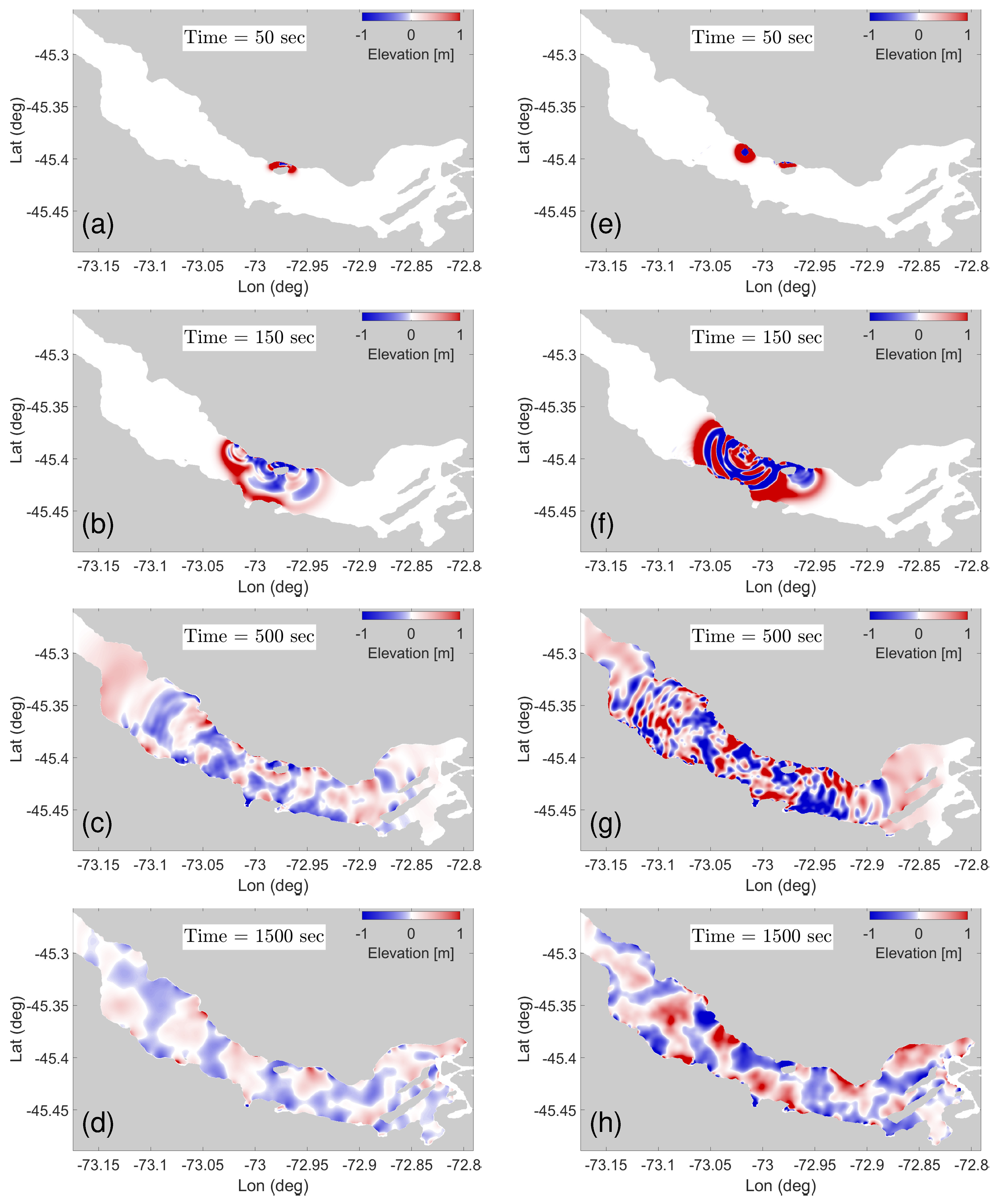
Figure 6 depicts the simulated tsunami wave propagation for the Aysén 2007 event, considering two models: (E1) a viscous fluid landslide and (E3) a solid landslide. A key distinction lies in the timing of the landslides. In the E3 model, both landslides enter the fjord simultaneously, unlike the staggered entry in E1. Furthermore, the E3 model exhibits larger tsunami wave amplitudes due to the non-deformable nature of the landslide (constant thickness throughout entry). This allows for a greater volume of material to enter the fjord, leading to higher waves. Additionally, a higher-frequency component is evident in the wave pattern generated by the E3 model (see
Figure 6g).
4.2. Maximum Water Elevation
This subsection analyzes the tsunami’s impact based on the maximum positive water surface displacement observed across all experiments E1–E6. This comparison aims to reveal how the different landslide types influence tsunamis.
Figure 7 reveals a significant difference in the maximum positive water surface tsunami between viscous and solid landslides. The impact generated for E1 and E2 are highly localized, whereas larger landslide volumes (
Figure 7e,f) naturally lead to higher free surface elevations compared to
Figure 7b,c. Additionally, comparing landslides with and without basal friction (e.g., E3–E4 and E5–E6) demonstrates that scenarios lacking basal friction exhibit a greater impact of the tsunami, reaching higher maximum elevations.
4.3. Run-Up Heights
This study presents a comparison between in situ measured run-up heights and those computed using numerical simulations (scenarios E1–E6). Complete run-up height results for all 21 observation points are available in
Section S2 of the Supplementary Materials. In this section, only the results corresponding to four selected observation points along the Aysén fjord are presented.
The analysis of
Table 5 reveals that scenarios E4 and E6 provide the most accurate representations of the observed data. Although E4 overestimates run-up heights in the vicinity of the PC and MI landslides, E6 aligns closely with the reference values. Scenarios E3 and E5 yield intermediate outcomes. It is significant that only scenario E4 slightly exceeds the maximum run-up measured by SERNAGEOMIN at Point 13, while underestimating the value relative to the observations reported by [
18,
33].
On the other hand, scenarios E1 and E2 show significant discrepancies with the reference data, especially E1. These underestimate run-up heights at most observation points, although overestimating some (e.g., Point 11 in E2). These differences could be attributed to local topographic effects, proximity to the simulated landslides, numerical model resolution, the parameterization of physical processes, and uncertainties inherent in field measurements.
4.4. Time Series
This subsection presents time series data for 6 of the 22 virtual tide gauges simulated along the Aysén fjord. For further reference, the remaining time series are included as
Supplementary Materials. We then focus on comparisons of simulated waveforms at the Chacabuco Port tide gauge, as it holds the unique distinction of capturing the 2007 Aysén tsunami. This analysis aims to estimate the landslide trigger time—determining the lag between the mainshock and the subsequent landslides.
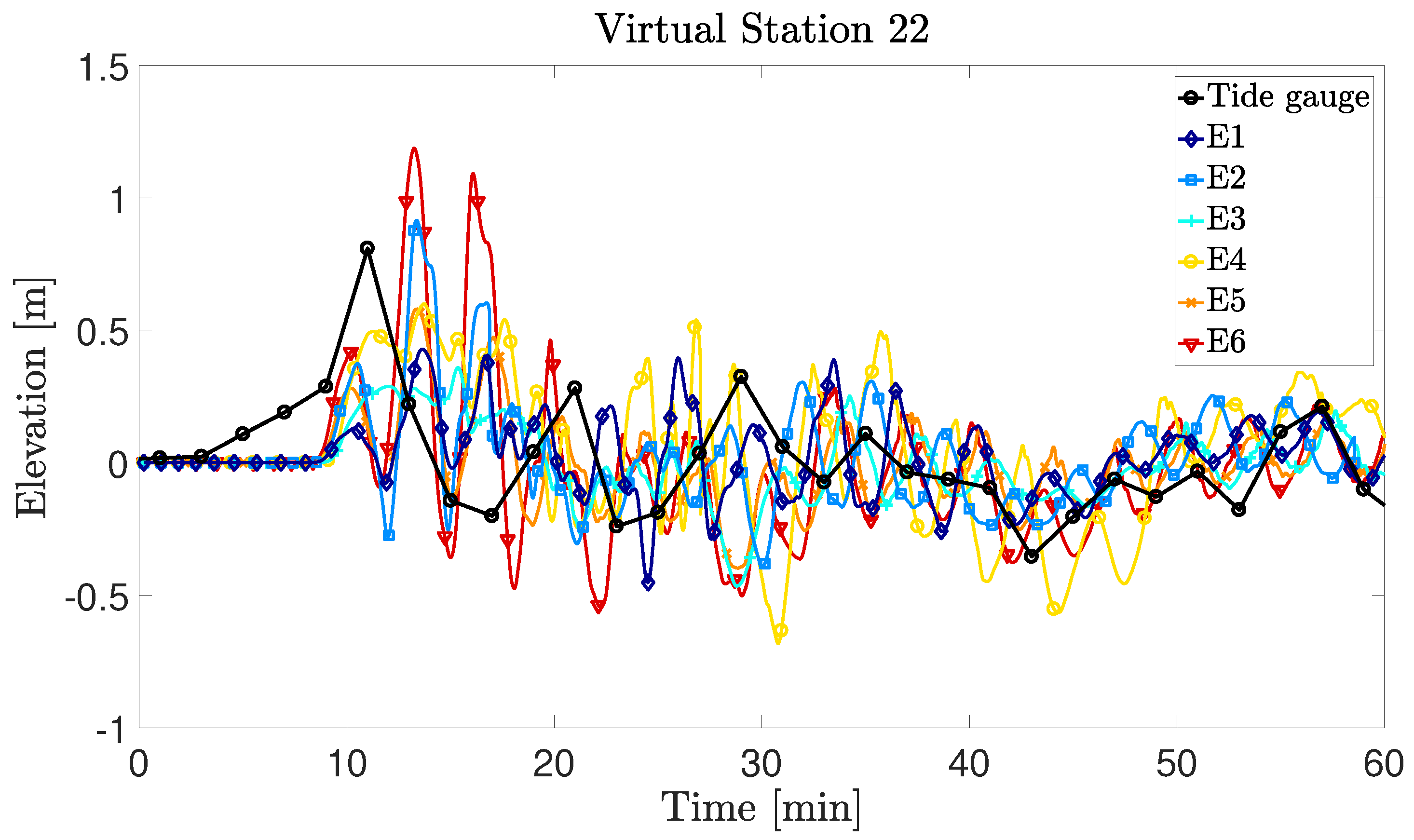
Figure 8b–d reveal a rapid decline in the absolute water surface amplitude. This behavior is characteristic of near-field tsunami waves, which are highly localized events. In contrast, far-field tsunamis exhibit smaller amplitude waves that travel in packets with a wider range of frequencies (frequency dispersion). Another interesting observation from
Figure 8 is the difference in arrival times (approximately 3 min) between Stations 1 and 22, despite their similar distances with respect to Station 13. This can be attributed to the presence of two islands in front of Chacabuco Port. These islands act as barriers, hindering the free movement of the waves and causing a delay in their arrival at the station.
Figure 9 presents a comparison between the time series simulated by experiments E1 to E6 and the recorded tsunami waveform at Chacabuco Port tide gauge. The 120 s sampling rate of the Chacabuco Port tide gauge limits a detailed comparison of the recorded waveform with the simulated signals from experiments E1–E6. While all models exhibit differences in amplitude, the most notable discrepancy lies in the initial 20 min of E3 and E4. These models show only positive amplitudes during this time window. This behavior can be attributed to the large distance between the source and the gauge. At such distances, the waves generated by subaerial landslides can undergo constructive interference, causing them to accumulate and manifest as a prolonged period of positive pressure.
To determine the time lag between the onset of the mainshock and the triggering of the PC and MI landslides, we conducted an additional experiment. To achieve this, we performed a cross-correlation analysis between the synthetic seismic signal at point 22 and the tide gauge record at Chacabuco Port (
Figure 9). However, the results obtained were counterintuitive, suggesting that the landslides were initiated before the main shock. While this apparent paradox could be attributed to uncertainties in the bathymetry used in the simulation or the high pre-existing stress levels in the fjord slopes, the available evidence does not support this hypothesis (see [
30]). The main limitation of this analysis was that the low sampling rate of the tide gauge (2 min) hindered the precise identification of the occurrence time of both events and led to a wide uncertainty window in the estimation of the time lag.
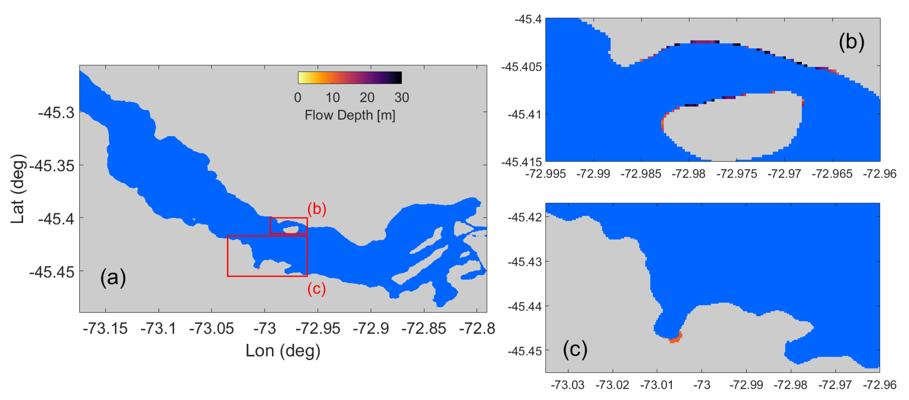
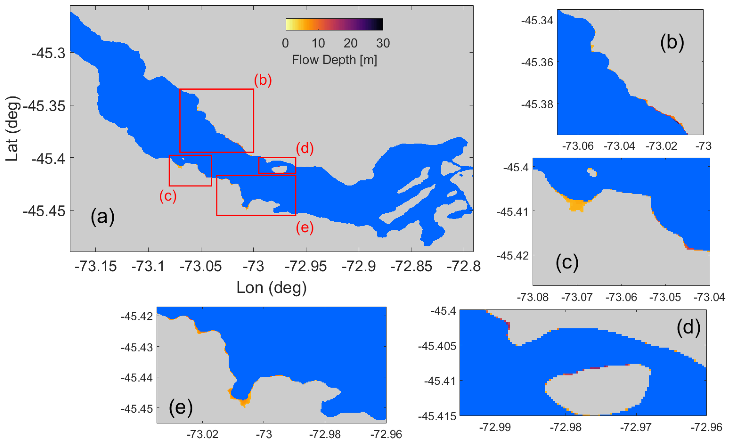
4.5. Inundation Zones
This final experiment presents the inundation areas in the Aysen Fjord produced by each of the six scenarios (E1–E6). The objective of this study is to analyze how the volume and rheological properties (viscosity or solid with Coulomb friction angle) of landslides affect the extent and location of inundated areas (see
Figure 10,
Figure 11,
Figure 12,
Figure 13,
Figure 14 and
Figure 15).
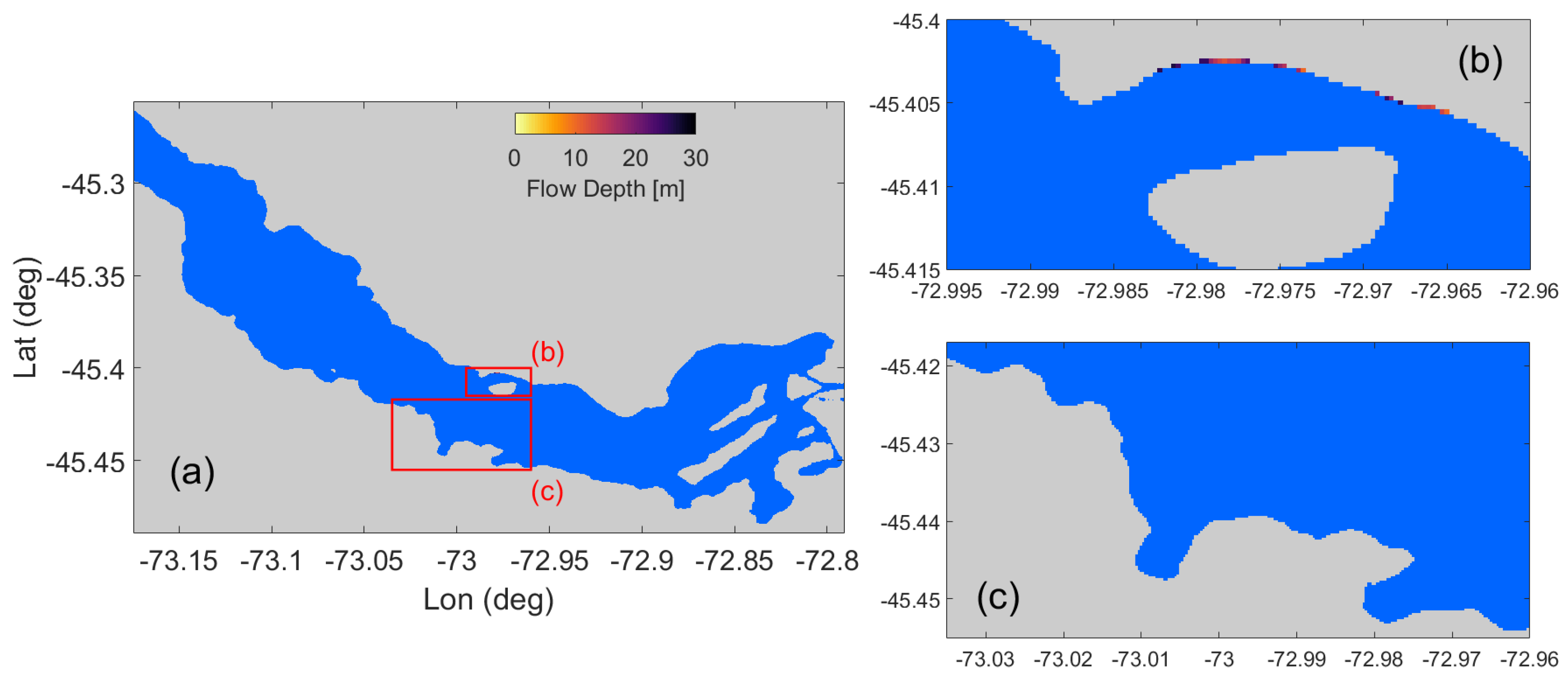
Figure 10,
Figure 11,
Figure 12,
Figure 13,
Figure 14 and
Figure 15 present the inundation zones resulting from the simulated tests. Red boxes highlight the areas of greatest interest in each figure. E1 proves to be the least destructive event, with a single inundation zone north of Mentirosa Island and a maximum estimated height of 10 m. As the magnitude of the volume landslide increases (E4 and E6), a significant increase in the extent and height of the inundations is observed. In these scenarios, wave heights greater than 30 m are recorded north of Mentirosa Island and close to 7 m south. In addition, a concentration of flooded zones is identified near the area enclosing points of observation 4 to 19, and outside this area, flood heights are less than 5 m (except for scenarios E4 and E6). These results demonstrate the strong influence of the volume of the granular landslide on the extent and severity of the inundations.
5. Discussion
Our simulations show a radial propagation of tsunami waves, following the same direction as the entry of the landslides into the Aysén Fjord. Since both landslides share the same entry direction, constructive interference occurs, amplifying the amplitudes of the generated waves. Furthermore, our results confirm the highly localized nature of these events, as the waves lose a significant portion of their amplitude in areas such as Puerto Chacabuco.
The impact of the tsunami associated with the landslides significantly depends on the rheology. Solid slides with a Coulomb friction angle generate a greater impact of the tsunamis compared to those with a viscous rheology (
Figure 7). This difference is attributed to a greater transfer of momentum from the solid slide with Coulomb friction angle to the water body, resulting in a more intense disturbance.
A distinctive pattern in all time series, especially at virtual stations located near the source, is a rapid decrease in the absolute value of the water surface elevation. This shows that the area near the source experienced a strong impact from the tsunami. While the water elevation in distant areas is lower, the interaction with the coast (reflection, for example) prolongs the wave propagation for several minutes. In addition, our simulations indicate that the arrival time of tsunami waves at the Chacabuco Port tide gauge is approximately 10 min, with scenarios E3 and E4 showing the best agreement with the tide gauge records (
Figure 9). The absence of detailed bathymetry and topography is a significant limitation. Our primary point of reference for assessing the impact of this data scarcity is the tide gauge record at Chacabuco Port (point 22,
Figure 3). The consistent failure of our six simulation tests to accurately reproduce the maximum water height and tsunami arrival time recorded at this gauge strongly suggests a crucial role for the lack of high-resolution bathymetry and topography in these discrepancies. However, isolating the specific contribution of each data limitation to the model inaccuracies remains a challenge without more detailed information.
The areas most vulnerable to inundation are located near the PC and MI landslides. Our analysis shows that the extent of these zones largely depends on the landslide type and the volume of material involved. Scenarios E5 and E6 exhibit the most extensive inundation zones. The results suggest that the landslide volume plays a crucial role in determining the magnitude of the inundation, although other factors such as the basal friction angle may also influence it.
Studies such as [
18] modeled the 2007 Aysén tsunami using COMCOT. However, by relying on the shallow-water equation, COMCOT is unable to capture the full spectrum of wavelengths present in this complex phenomenon, especially those associated with tsunamis generated by subaerial landslides. Unlike these studies, our model, which considers solid with Coulomb friction angle and viscous landslides, allows for a more realistic simulation of tsunami propagation and captures higher wave heights. When comparing our results to those of [
18], we notice an overall similarity in the maximum sea surface elevation. However, the use of granular landslides in our simulations produces higher maximum wave heights, unlike the results obtained when considering viscous landslides. A novel contribution of our work is the generation of the synthetic time series for Chacabuco Port, enabling a more detailed comparison with future observations. Additionally, our model allows us to analyze how the rheology of the landslide influences the energy transmitted to the Aysén fjord.
While our model, the first to simulate the 2007 Aysén tsunami without using codes based on the shallow-water equations, presents several limitations, such as the lack of detailed bathymetry and topography, the assumption of a solid slide with a slab geometry, and the simulation’s initiation independent of the earthquake, offers an initial approximation to understand the areas affected by the tsunami in the Aysén Fjord. Additionally, modeling the landslides with a uniform rheology and the limitation of NHWAVE to three vertical grids impose significant computational constraints. Despite these limitations, which can be addressed in future research, our results provide a solid foundation for more detailed studies on landslide-generated tsunamis in the fjords of southern Chile.
While research since 2013 has consistently shown that solid block landslides tend to overestimate wave characteristics and generate larger waves than deformable landslides, ref. [
43] offered a notable exception [
13]. Ref. [
43] proposed that block slide may generate larger, identical, or even smaller waves than granular slides based on comparing landslide-generated waves characteristics estimated by their formulations, developed based on 144 experiments on rigid blocks, and the published equations of [
44] for granular slides. This finding underscores the importance of considering landslide deformability, as, despite our results aligning with those obtained by most investigations, the opposite case remains a possibility.
6. Conclusions
In this study, we used the NHWAVE and FUNWAVE-TVD numerical models to simulate the 2007 Aysén tsunami. We focused on the landslides at Punta Cola and north of Mentirosa Island, considered the primary triggers of the event. We assume a co-occurrence of PC and MI landslides and model them under two approaches: as viscous fluids (deformable) and as granular solids (undeformable). We employed a rigid slab geometry model to simulate the Aysén tsunami under two main scenarios. In the first scenario, we incorporated rheological parameters specific to the Aysén fjord or Chilean Patagonia to represent local conditions. In the second scenario, we explored an extreme case with no basal friction, similar to conditions that have been investigated in other studies (see [
40]). With the viscous model, we aim to approximate the real-world conditions of the event, modeling the landslide as a debris flow, using in situ rheological parameters.
NHWAVE proved to be ideal for modeling the generation and propagation of landslide-generated tsunamis due to its reliance on the Navier–Stokes equation. This equation imposes no restrictions on wavelength, allowing for an accurate representation of dispersion phenomena and other second-order effects. On the other hand, FUNWAVE-TVD, while significantly reducing computational time, is limited to modeling the propagation of the tsunami once generated.
Both landslide volume and Coulomb internal friction angle significantly influence the amplitude of the generated waves, according to our results. These findings are consistent with previous studies, such as [
36] and highlight the importance of considering both parameters in modeling landslide-generated tsunamis. Uncertainty in landslide volume estimation represents a significant challenge in tsunami modeling. As demonstrated by the different values reported for the Aysén event in the literature (
Table 3 and
Table 4), variability in these estimates can lead to very different results in numerical simulations. This underscores the importance of having detailed geophysical data and accurate estimation methods to assess the risk of landslide-generated tsunamis.
The 2007 Aysén tsunami marked a milestone in the understanding of coastal risks in Chile. This event demonstrated conclusively that subaerial landslides are capable of generating devastating tsunamis, thereby expanding the spectrum of coastal threats beyond traditional earthquakes. The Aysén experience raised greater awareness of the need to consider this type of event in risk assessments and in the planning of civil protection measures, especially in regions with rugged topography and high susceptibility to landslides.
In the future, this methodology will enable a more accurate assessment of the disaster risk associated with tsunamis generated by subaerial landslides in fjord, coastal, or lacustrine environments. This will facilitate the implementation of more effective mitigation measures to protect the areas exposed to these types of events.


