Article

Coastal Dynamics Analysis Based on Orbital Remote Sensing Big Data and Multivariate Statistical Models

by
Anderson Targino da Silva Ferreira
1,2,3,4,*,
Regina Célia de Oliveira
3,
Maria Carolina Hernandez Ribeiro
5,
Carlos Henrique Grohmann
6 and
Eduardo Siegle
4
1
Department of Geoenvironmental Analyses, University of Guarulhos, Guarulhos 07023-070, Brazil
2
Technology in Environment and Water Resources, São Paulo State Technological College of Jahu, Jaú 17212-599, Brazil
3
Department of Geography, Institute of Geosciences, State University of Campinas, Campinas 13083-855, Brazil
4
Oceanographic Institute, University of São Paulo, São Paulo 05508-120, Brazil
5
School of Arts, Sciences and Humanities, University of São Paulo, São Paulo 03828-000, Brazil
6
Institute of Energy and Environment, University of São Paulo, São Paulo 05508-010, Brazil
*
Author to whom correspondence should be addressed.
Coasts 2023, 3(3), 160-174; https://doi.org/10.3390/coasts3030010
Submission received: 1 May 2023 / Revised: 19 June 2023 / Accepted: 26 June 2023 / Published: 29 June 2023
(This article belongs to the Special Issue Measuring Shoreline Variability and Understanding It's Local Impacts)

Abstract

:
As the interface between land and water, coastlines are highly dynamic and intricately tied to the sediment budget. These regions have a high functional diversity and require enlightened management to preserve their value for the future. In this study we assess changes to the São Paulo State (SE Brazil) coastline over the last 36 years. The study innovatively employs big data remote sensing techniques and multivariate statistical models to evaluate and generate erosion/accretion rates (1985–2021) relative to beach orientation and slope. Shoreline change rates have been obtained for sandy beaches at 485 one-kilometer-spaced transects. Our findings capture the complexity and heterogeneity of the analyzed coastline, at a regional and local scale. No association was found between shoreline changes and beach face orientation. Nonetheless, a dependency relationship was found between dissipative beaches with moderate to high accretion. Beaches facing south, with relative stability, were prone to sediment accumulation. Locations with slow accretion, like sandy spits and tombolo-protected beaches, were associated with dissipative beaches with moderate to high accretion. The southeast-oriented beaches are more prone to erosion due to storm waves from the south. Results provide a broad, fast, and relatively low-cost methodology that can be used in any sandy beach context, bringing essential information for coastal management and decision-making related to the use and occupation of the coastal zones.

1. Introduction

Climate change refers to the alteration (cooling or heating) of Earth’s atmospheric temperature and its ensuing implications (i.e., extreme events). These shifts can occur due to natural forcings such as variations in solar activity, alterations in the Earth’s orbital characteristics (Milankovitch Cycles), and volcanic eruptions (which cause a reflection of solar radiation followed by subsequent cooling). Anthropogenic, or human-caused changes, can excessively introduce greenhouse gases (GHGs) into the atmosphere. These gases contribute to global warming by blocking the escape of radiated heat and causing, among other issues, polar ice melt, changes in atmospheric circulation, oceanic circulation, and the hydrological cycle [1,2,3,4].
In coastal zones, these changes increase the Mean Sea Level (MSL), currently at 3.55 mm/year [5,6,7]. According to projections from the International Panel on Climate Change (IPCC), this could reach up to 1.2 m by 2100 under the most pessimistic scenario (SSP5—8.5) [2,3]. The rise in MSL, along with the impact of waves, currents, and tides, add to the erosion rates of the Shoreline (SL), which are amplified by these extreme events [3,8,9,10,11]. This process exerts synergistic/chaotic effects on the environment and human activities in the coastal zone, primarily by destroying infrastructure and natural areas. Consequently, it affects the safety of populations living near the coast and economic activities such as tourism and damages biodiversity and coastal ecosystems [7,12,13,14,15].
This projection makes adapting to climate change and its impacts increasingly urgent. This underscores the importance of developing methodologies for obtaining precise, large-scale data as quickly as possible to assess populations’ exposure to these risks [16]. In this context, orbital remote sensing (RS) and machine learning-based techniques can support large-scale coastal ecosystem modeling at a relatively low cost and with spatial and temporal resolution suitable for main applications in coastal zones [17,18,19,20], such as rapid update monitoring. This stands in contrast to classic surveys using water level hoses, geometric leveling, and polygonation [17,18,19]; global navigation satellite systems [20,21,22]; and aerial photogrammetry or laser scanning with light detection and ranging on land platforms, as well as in manned or remotely piloted operations [23,24,25].
Previous works have brought advances in studying coastal dynamics [26,27] and beach slopes [28] based on satellite images. However, the present research is innovative by providing an integrated assessment of parameters such as erosion/accretion rate; orientation, and beach slope, derived from the combination of different orbital sensors and multivariate statistical models, which are unsupervised and applicable in any context of sandy beaches. This is accomplished through free, open-access computational platforms (e.g., Google Earth Engine—GEE).

2. Materials and Methods
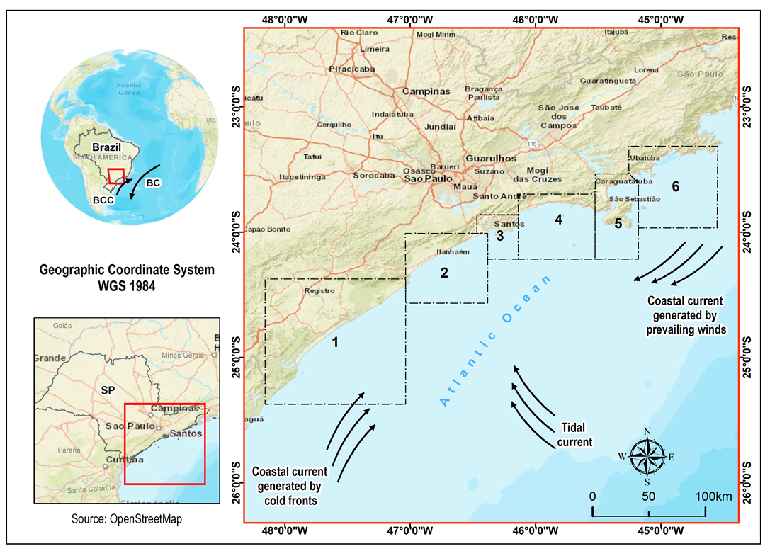
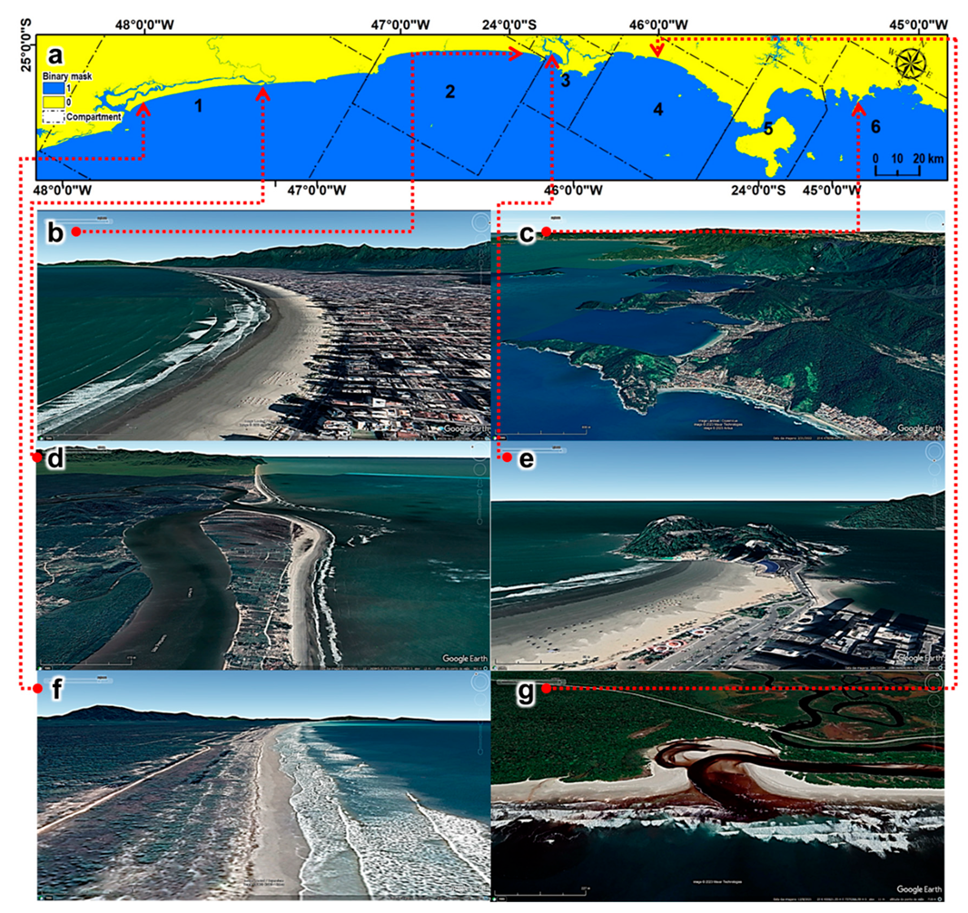
2.1. Study Area

The ~600 km long coast of São Paulo State (SE Brazil) is divided into six compartments, which are: (1) Ilha do Cardoso–Serra do Itatins; (2) Peruíbe–Praia Grande; (3) Santos–Bertioga; (4) Bertioga–Toque-Toque; (5) Toque-Toque–Tabatinga; and (6) Tabatinga–Picinguaba (Figure 1), according to Tessler et al. [29]. Its physiography presents a variety of geomorphological features, such as beaches, rocky shores, sandbars, and mangroves. It is marked by a complex interaction between geological, geomorphological, climatic, and anthropogenic processes.
Some of these features (i.e., vegetated areas, mangroves, sandy beaches, and rocky shores) are common on the southern part of the coastline. The flatter topography includes ecologically essential areas, such as the Juréia-Itatins and Itinguçu State Park [29,30]. In this portion of the coastline, the Serra do Mar escarpment appears farther from the coast (10 km–70 km), creating room for a broad coastal plain with long, straight beaches and some islands [29,31].
From the central portion to the northernmost part, the Serra do Mar Mountain chain range gradually approaches the coast, generating a narrow coastal plain and smaller hydrographic basins, when compared to those in the southern portion of the São Paulo coast. This part of the coast is geomorphologically more irregular, with smaller and more sheltered beaches in the form of coves, separated by pre-Cambrian rocky promontories such as those observed at Itaguaré, Massaguaçu, and Praia Vermelha do Norte [29,31]. This region is home to important cities such as Santos, which has the largest port in Latin America [32]. While the northern coast has sandy beaches in pockets between rocky outcrops and presents a more rugged topography, with the presence of the Serra do Mar and dozens of islands near the coast [33].
The circulation of the Brazilian continental margin is dominated by the Brazil Current (BC), which flows southwards in deep waters. Meanwhile, the Brazil Coastal Current (BCC) moves from the south-southeast to the northeast on the continental shelf during spring and winter [34,35,36] (Figure 1). The prevailing winds are from the east-northeast, generating currents parallel to the northeast-southwest coastline. However, under the influence of cold fronts, frequent during winter, winds from the south-southeast generate more intense currents and waves coming mainly from the southern quadrant [22,37,38,39,40] (Figure 1). Urban occupation and the construction of coastal infrastructure also significantly impacts the coastal physiography and dynamics, which can result in erosion and progradation processes [41,42].
Figure 1. Location of the compartments on the São Paulo coast: (1) Ilha do Cardoso–Serra do Itatins; (2) Peruíbe–Praia Grande; (3) Santos–Bertioga; (4) Bertioga–Toque-Toque; (5) Toque-Toque–Tabatinga; and (6) Tabatinga–Picinguaba. (BCC = Brazil Coastal Current, BC = Brazil Current). Source: modified from Ref [29,40].
Coasts 03 00010 g001

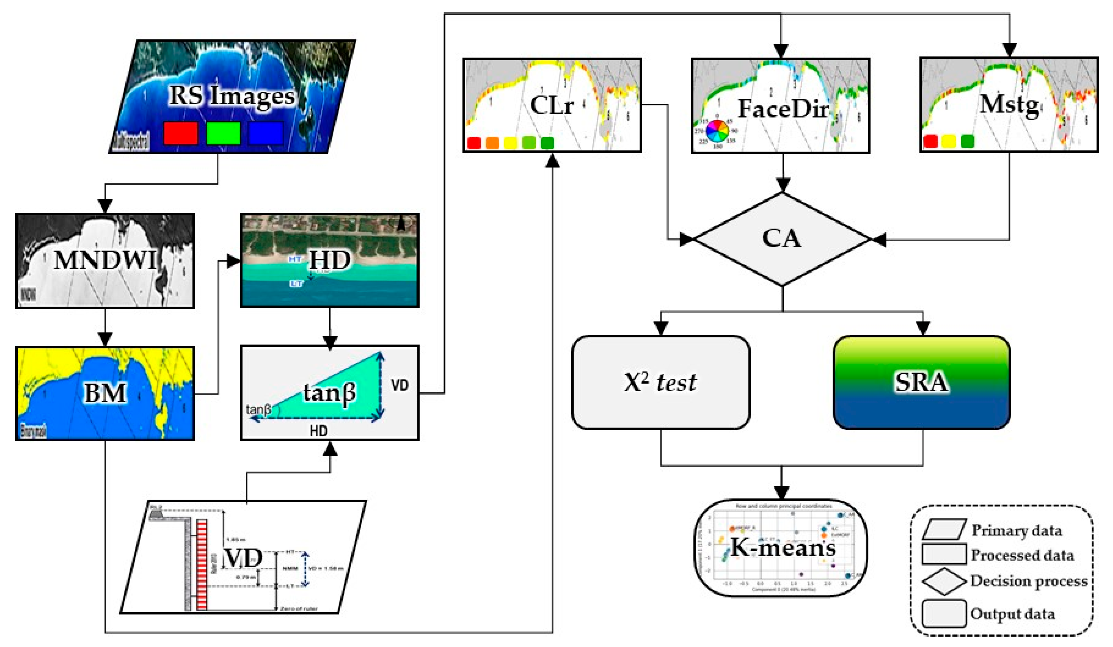
2.2. Processing Steps

The methodology of this research is divided into three steps: (1) acquisition of orbital remote sensing images for the generation of the modified normalized difference water index (MNDWI), binary mask (BM), and slope parameter (tanβ) derived from horizontal (HD) and vertical (VD) distances; (2) generation of maps of the annual erosion and accretion rate (CLr), beach face direction (FaceDir), and morphodynamic stage trend (Mstg); (3) analysis of associations, dependency relationships, and clusters by correspondence analysis (CA), chi-square test (X2), standardized residual analysis (SRA), and cluster (K-means) (Figure 2).

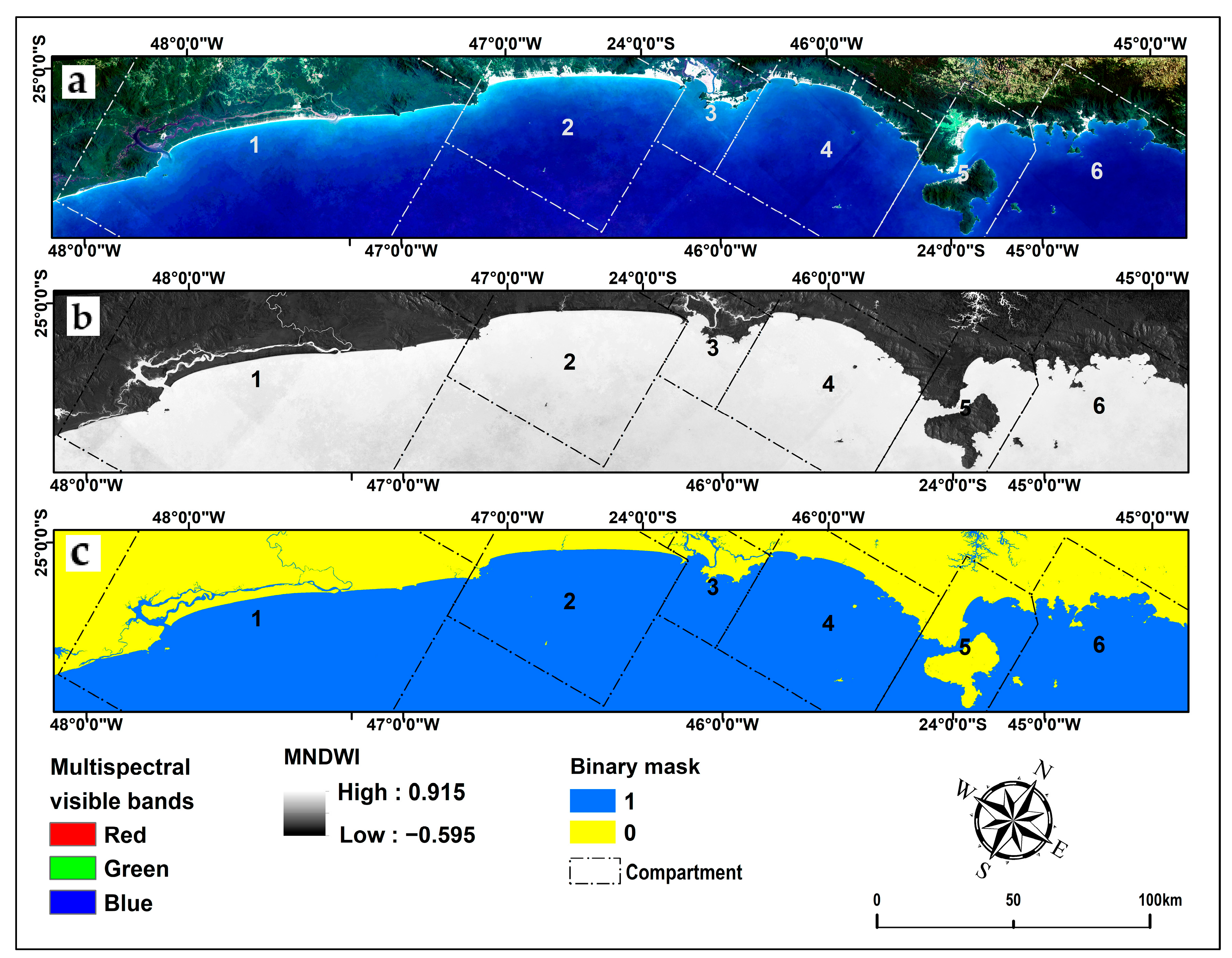
2.2.1. Orbital Remote Sensing Images
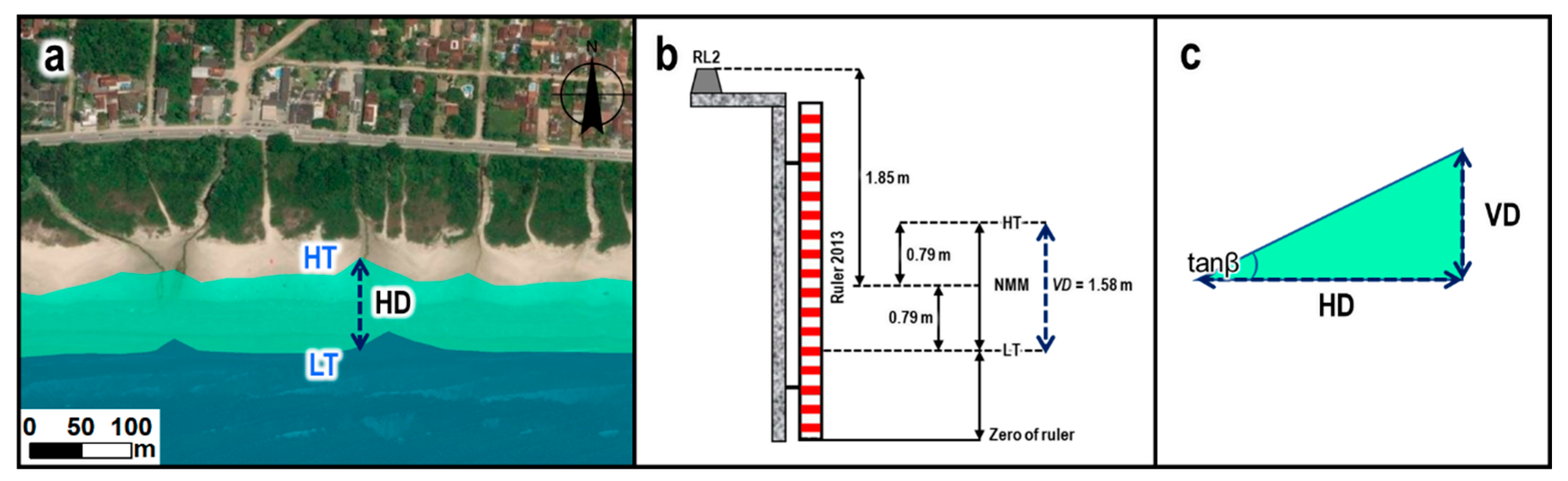
This study uses annual medians of Landsat 5/TM and Landsat 8/OLI multispectral satellite/sensor images for 1985 and 2021. These images have a spatial and temporal resolution of 30 m and 16 days respectively, with calibrated top-of-atmosphere (TOA) reflectance acquired by the Google Earth Engine (GEE) platform [43,44,45,46,47,48] (Figure 3a). The water/non-water (or land) interface was mapped using the Modified Normalized Difference Water Index (MNDWI) [49] (Figure 3b), calculated for each year using a binary mask (water “1” and non-water “0” classes) with a spatial mode filter to eliminate noise [50] (Figure 3c).
The assessment of the accuracy of the “water” and “non-water” area map classification was carried out using the analytical technique of global accuracy (GA) and global error (GE) indices, represented respectively by Equations 1 and 2. This was implemented based on the percentage of correctly classified samples from the total available samples, as well as the overall percentage error of the matrix [51].
G A = V T × 100
G E = 100 A G
V represents the correctly classified values, and T represents available samples.

2.2.2. Database

The coastal erosion and/or accretion rate (CLr) was derived from the difference between the reference year (1985) and the current analyzed year (2021) positions. This was achieved using binary masks and the intersection of equidistant transects (1 km × 1 km), with Landsat 5 and 8 satellites as the base reference [52]. Quantitative variables were transformed into qualitative ones and standardized according to the nature of the data.
Thus, according to Thieler and Hammar-Klose [53], the CLr values were transformed into the following intervals: high erosion—HEr (<−2.0 m); moderate erosion—MEr (−1.0 m–−2.0 m); stable—Stb (−1.0 m–1.0 m); average accretion—MAc (1.0 m–2.0 m); and high accretion—HAc (>2.0 m). The beach face direction (FaceDir) was determined by the transect direction relative to geographic north as follows: north—N (0°–22.5°); northeast—NE (22.5°–67.5°); east—E (67.5°–112.5°); southeast—SE (112.5°–157.5°); south—S (157.5°–202.5°); southwest—SW (202.5°–247.5°); west—W (247.5°–292.5°); northwest—NW (292.5°–337.5°); north—N (337.5°–360°) [54].
The slope model (tangβ in Equation (3)) was derived from the horizontal (HD) and vertical (VD) distances, respectively, between the differences between high and low tide coastlines (CL) (Figure 4a) and from the spring tide range. For example, near the Port of Santos (the central point of the study area), the average spring tide range is 1.58 m (Figure 4b), according to the Mean Sea Level (MSL) of the Imbituba/SC datum of the Brazilian Geodetic System (BGS) [22,55].
tanβ = atan(VD/HD)
HD was obtained from multispectral remote sensing (RS) harmonized between Landsat 8 and Sentinel-2 (HLS) images, resampled to 30 m spatial resolution (Figure 4a) for the years 2019 and 2021. This technique can improve temporal resolution by up to 7 scenes per month at the exact location [56]. The median HSL images were acquired synchronously between satellite pass time (~10:30 A.M.) and high and low spring tide stages, obtained through the WXTIDE32 software [57]. This resulted in two High Tide (HT) and Low Tide (LT) images from the median of 26 HT images and another of 27 LT images covering the entire study area. The satellite-derived slope information (Figure 4c) provides a rapid empirical assessment of the morphodynamic beach stage (Mstg) trend, which can be divided into: steeper—ST (0.12 < tanβ); intermediate—IN (0.05 < tanβ < 0.12), and sloping—SL (tanβ < 0.05) [28,58].
Figure 4. Shows three parameters: (a) the Horizontal Distance (HD) between the coastlines of Spring High Tide (HT) and Low Tide (LT), which was derived from satellite images; (b) The Vertical Distance (VD) of the tidal range near the port of Santos, São Paulo, Brazil [55,57] and (c) The slope (tanβ) of the right triangle formed by the horizontal and vertical distances.
Coasts 03 00010 g004

2.2.3. Multivariate Statistical Models

The satellite-derived slopes were statistically calibrated using 24 topographic profiles collected in situ through the positioning of the Global Navigation Satellite System (GNSS) and a Box-Cox transformation regression model, which maximizes the adherence of the new variable’s distribution to normality [22,28,59,60,61,62]. Correspondence analysis (CA) examined dependency relationships due to associations between categories of the variables of interest using the chi-square (X2) test. Meanwhile, standardized residual analysis (SRA) assessed the existence of interdependence relationships between these categories based on the reference critical value (+1.96≤) of the standard normal curve, with a significance level of 5%. Thus, if the adjusted standardized residual value in a cell is greater than 1.96, it is interpreted that there is a significant association between these categories [61,63,64].
Cluster analysis using the non-hierarchical K-means method employs the coordinates of the rows and columns of the contingency table, grouping their observations based on centroid proximity in a perceptual map. The advantage of this method is that it can be applied to samples with large amounts of data [61,62]. To this end, the Elbow method was employed to select the number of clusters [61,62,64,65,66].

3. Results

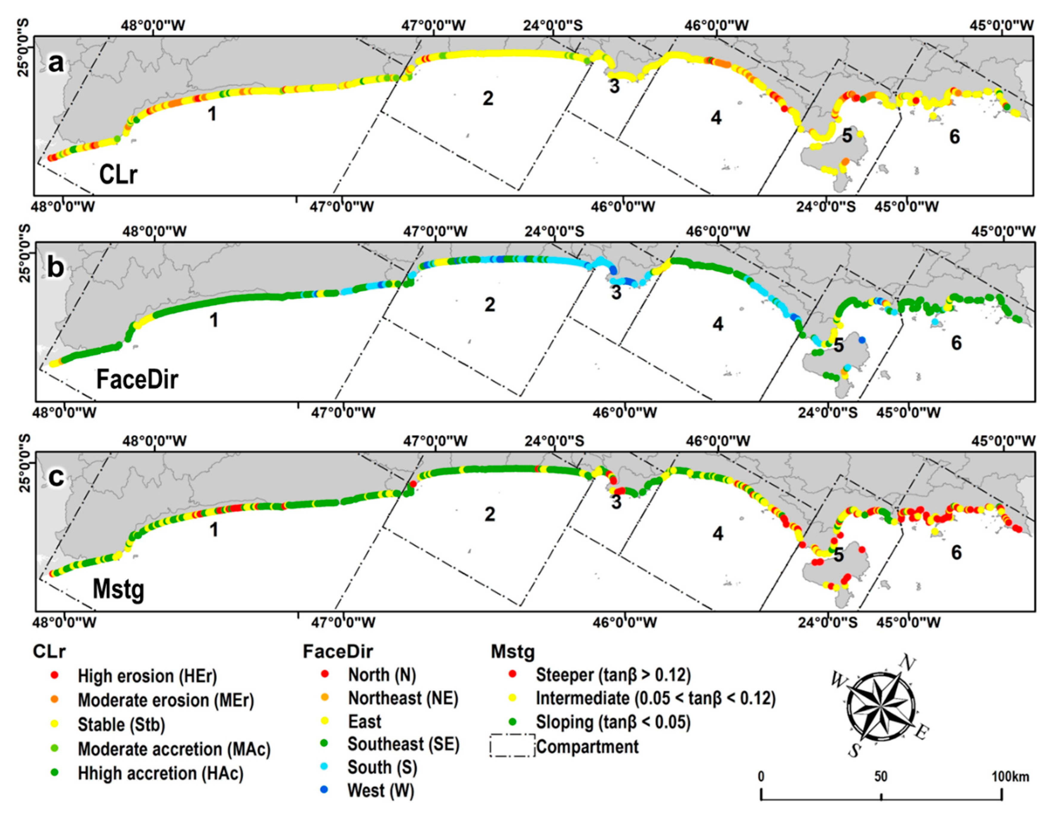
3.1. Description and Geographic Distribution

The calibration between the slope estimated by satellite and that measured in situ exhibited a coefficient of determination of 0.94 (R2) and a root-mean-square error of 0.18 (RMSE). This indicates that the slope values collected in the field explain approximately 94% of the variance in the satellite-derived data [67]. Furthermore, orbital imagery acquired between 1985 and 2021 demonstrated a global accuracy and global error in mapping the land/sea boundary of 99% and 1%, respectively. These results underscore that the classification is suitable for this type of study.
The 485 transects perpendicular to each kilometer of the unconsolidated coastline exhibited an average CLr of −0.17 m, with minimum and maximum values of −70.1 m and 103.4 m, respectively. The beach faces displayed an average direction of 148° (SE), with values ranging from 16° (N) to 264° (W). The slope of these faces was predominantly intermediate on average.
Table 1 shows the statistical summary for each compartment of the São Paulo coast. The first, Ilha do Cardoso–Serra de Itatins (C1), has a moderate and positive CLr, with more erosive areas in its central-southern portion and accretion in its northernmost portion (Figure 5a). In this compartment, as well as in the others, the direction of the beach face is predominantly SE. However, the average slope of C1 is less than 0.05, indicating a tendency towards a dissipative morphodynamic state. From the Peruíbe–Praia Grande compartment (C2) onwards, the scenario of the average CLr becomes negative and worsens in the Tabatinga–Picinguaba compartment (C6). While the average slope values remained below 0.05 until compartment C2, they gradually increased, becoming intermediate in compartments C3 and C4 (0.05 < tanβ < 0.12), as well as reflective in compartments C5 and C6 (tanβ > 0.12).
Transects with moderate and high erosion (MEr and HEr) were observed in greater proportion in compartments C1, C4, and C5. In contrast, they were observed in a smaller proportion in compartments C2 and C6. Compartment C3 did not exhibit erosive processes. In these compartments, southeast-facing (SE) beach faces predominate (Figure 5a). Beaches with faces oriented southward appear primarily in the northern portion of compartments C2 and C4 and throughout compartment C3 (Figure 5b). Beaches with a shore trend (ST) and indeterminate (IN) orientation predominate in compartments C1 through C4, with sloping profiles primarily occurring in compartments C5 and C6 (Figure 5c).

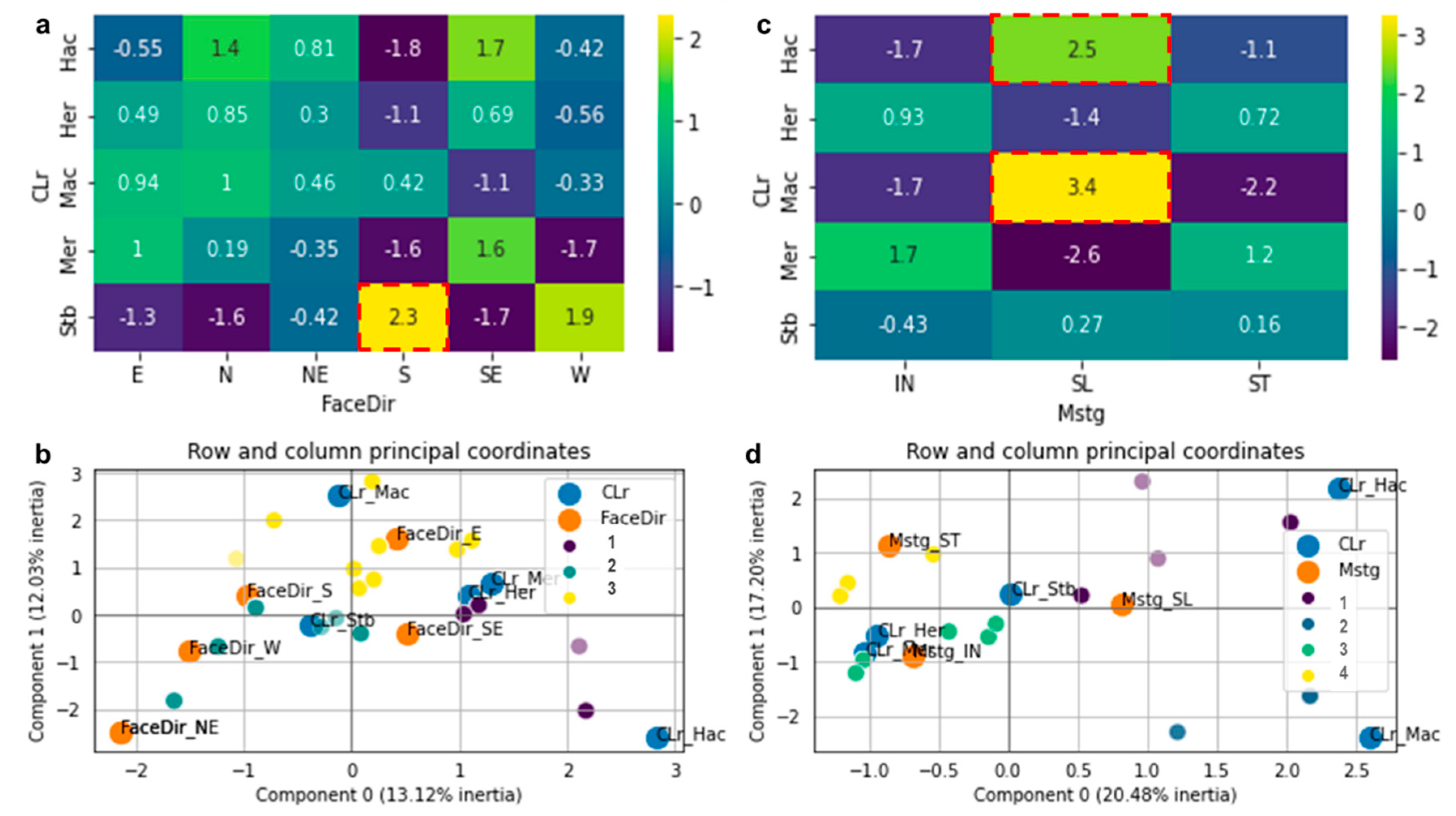
3.2. Associations, Dependency Relations, and Clusters

Through Correspondence Analysis (CA), the Chi-square (X2) test found a p-value of 0.4153, suggesting the hypothesis that there is no statistical significance (H0, p-value > 0.05) or association between the variables of the annual erosion and/or accretion rate (CLr) with the direction of the beach face (FaceDir). However, the adjusted standardized residuals (ASR) observed a dependency relationship between relatively stable beaches (Stb) with beach faces facing the S quadrant (1.96≤; red dashed cell in Figure 6a). The remaining cells in Figure 6a indicated random or statistically non-significant processes between CLr and FaceDir (values < 1.96). For the same variables (CLr and FaceDir), Figure 6b of the K-means Cluster analysis identified three different groupings. The first (cluster 1) observed SE-facing transects with beaches with moderate and high erosion (CLr_MEr and CLr_HEr). The second (cluster 2) indicated E-facing beach faces grouped with those having moderate accretion rates (CLr_MAc). Cluster 3 grouped stable transects (CLr_Stb) with beach faces facing S, W, and NE (Figure 6b).
For the variables of CLr and morphodynamic state (Mstg), the X2 test observed a statistically significant association with a p-value of 0.0017 (H1, p-value < 0.05). The analysis of the ASR values observed that beach faces with dissipative characteristics (ST) exhibited a dependency relationship (1.96≤) with transects of moderate and high accretion (MAc and HAc) (red dashed cells in Figure 6c). For the same variables (CLr and Mstg), Figure 6d of the K-means Cluster analysis found four different groupings. Transects with moderate and high accretion (CLr_MAc and CLr_HAc) appear grouped in clusters 1 and 2 close to beaches with a dissipative tendency (Mstg_ST). In Figure 6d, beaches with relative stability (CLr_Stb) appear grouped at the center of the perceptual map, orbiting with relative equidistance from the different Mstg categories. In the third cluster, transects with moderate and high erosion (CLr_MEr and CLr_HEr) appeared preferentially grouped with beaches having an intermediate morphodynamic tendency (Mstg_IN). Meanwhile, cluster 4 orbits beaches with a reflective tendency (Mstg_SL) closer to transects with moderate erosion (CLr_Mer), high erosion (CLr_HEr), and stability (CLr_Stb).

4. Discussion

Global-scale studies such as those by Luijendijk et al. [26] and Mentaschi et al. [27] can provide an overview of coastal erosion or accretion processes by identifying global trends and patterns. However, such global approaches cannot capture the complexity and heterogeneity of coastal environments at a regional or local scale.
In this context, along the São Paulo coast, beaches with relative stability oriented toward the southern quadrant displayed sectors that are more susceptible to accretion processes. This is due to the ~90° angle between storm waves formed by cold fronts coming from the same quadrant, which results in these beaches having their sediment transport almost nullified (Figure 7a), favoring sediment accumulation and, consequently, the formation of frontal dunes in these areas [22,38,68]. In addition, beaches with facies oriented towards E, W, and NE, impacted by lower-energy waves from ENE during summer or protected by oceanic islands, also favor sediment accumulation.
However, it is essential to note that along the São Paulo coast, these beaches (oriented towards E, W, and NE) are small and underdeveloped, primarily found in C5 and C6 (Figure 7c), where the proximity of the Serra do Mar Mountain chain provides a heavily indented coast with bays and inlets separated by rocky promontories (Figure 7b) [29,68]. This configuration may favor significant negative changes in sediment volume due to climate change-related global warming, which has increased wind speed and wave height [69,70], intensifying cyclonic and anticyclonic events in the Southern Hemisphere as well as their trajectories, intensity, and frequency during winter months [71,72]. Furthermore, particularly in C5 and C6, anticyclones may generate high-energy ENE waves, causing erosion on these similarly-oriented beaches [73].
Beaches with dissipative tendencies and moderate to high accretion are associated with locations characterized by slow accretion processes, such as sandy spits and areas protected by tombolos (Figure 7c,d), respectively, in compartments C1 and C3 [29,74,75,76]. Due to the São Paulo coast’s configuration (SW-NE), beach faces oriented toward SE are more susceptible to erosive processes, as the acute angle (~45°) of storm wave incidence from the same Southern quadrant can reach up to 4.0 m [20,22,38,40,77] during the austral autumn and winter (April to September), favoring maximum sediment transport capacity (e.g., [78,79]). This process is typical on straight beaches found in the south-central portion of compartment C1 (Figure 7e) and on those with intermediate and steeper tendencies in compartments C4, C5, and C6 of Figure 5c [74,80]. Meanwhile, dissipative beaches associated with moderate erosive processes are located near river mouths, estuaries, and tidal channels, naturally dynamic regions in Figure 7f [29].
These sites may undergo drastic changes, such as the disappearance of beaches due to rising sea levels, the intensification of extreme events, and human activities [81,82]. Such changes may induce regime shifts and collapse of social-ecological systems, with negative implications for biodiversity and ecosystem services [83,84,85]. However, Cooper et al. [86] caution that one should be wary of these projections, given that sandy beaches are highly resilient environments and, if space is available, they can adapt through sediment redistribution, such as those found in the central-northern portion of C1 (Figure 7d).
Nonetheless, not all beaches will be capable of adapting, making coastal conservation and management measures essential [86]. This is particularly true in urbanized areas, such as the easternmost portion of the beachfront in Santos near the eponymous canal and port (C3), which experiences frequent flooding due to storm surges [20,77]. This highlights the importance of integrated and collaborative approaches among governments, communities, and scientists to address coastal erosion and ensure the safety of coastal communities [87].
Lastly, this work may serve as background information for future studies on the deposition and accumulation of microplastics, given that naturally sediment-prone sites (i.e., accretion) along the São Paulo coast are described as susceptible to this pollutant’s accumulation, such as pellets [22]. This research contributes to the fulfilment of Sustainable Development Goal 14 (life below water), more specifically of targets 14.1—which aims to prevent and significantly reduce marine pollution of all types, in particular from land-based activities, including marine debris (indicator 14.1.1—density of plastic waste) by 2025—and 14.a, which aims, among others, to increase scientific knowledge, develop research capacities, and transfer technology to improve the health of the oceans [88].

5. Conclusions

The analysis of orbital images from the coast of São Paulo in 1985 and 2021 allowed the assessment of the annual rate of erosion and accretion along the 485 transects distributed perpendicularly to the coastline at each kilometer of sandy beaches. Therefore, the overall accuracy and global error of the land/sea boundary mapping were deemed suitable for the study. From compartments C1 to C6, a general trend of dissipative morphodynamic state was observed, except for compartment C2, where the intermediate state predominated. Furthermore, beaches oriented towards the southeast were most affected by erosive processes. In contrast, the beaches with dissipative tendencies and moderate to high accretion were associated with locations characterized by slow accretion processes. Furthermore, a dependency relationship was observed between relatively stable beaches facing the southern quadrant and transects with moderate to high accretion. Overall, the results provide essential information for coastal management and decision-making related to the use and occupation of the São Paulo coastline, especially about the accumulation of microplastics. This study contributes to the fulfilment of Sustainable Development Goal 14 (life below water), specifically of target 14.1 with respect to marine debris, scientific knowledge, and investigation. Lastly, it is recommended to include new parameters that may influence the variation of the coastline and aid in better understanding the coastline its behavior, such as the distance of transects to urbanized areas, rocky promontories, oceanic islands, and channels/estuaries.

Author Contributions

Conceptualization, A.T.d.S.F., R.C.d.O., M.C.H.R. and E.S.; methodology, A.T.d.S.F., R.C.d.O., C.H.G. and E.S.; validation, A.T.d.S.F., R.C.d.O., C.H.G., M.C.H.R. and E.S.; formal analysis, A.T.d.S.F., R.C.d.O., C.H.G., M.C.H.R. and E.S.; investigation, A.T.d.S.F., R.C.d.O. and E.S.; resources, A.T.d.S.F., R.C.d.O. and E.S.; data curation, A.T.d.S.F. and E.S.; writing—original draft preparation, A.T.d.S.F., R.C.d.O., C.H.G., M.C.H.R. and E.S.; writing—review and editing, A.T.d.S.F., R.C.d.O., C.H.G., M.C.H.R. and E.S.; supervision, A.T.d.S.F., R.C.d.O. and E.S.; project administration, A.T.d.S.F.; funding acquisition, A.T.d.S.F., R.C.d.O. and E.S. All authors have read and agreed to the published version of the manuscript.

Funding

This study was partially funded by the São Paulo Research Foundation (FAPESP grant #2020/12050-6). E.S. (#308229/2022-3), R.C.O. (#306931/2022-2), and C.H.G. (#311209/2021-1) are National Council for Scientific and Technological Development (CNPq) research fellows.

Institutional Review Board Statement

Not applicable.

Informed Consent Statement

Not applicable.

Data Availability Statement

Acknowledgments

The authors thank the Oceanographic Institute of the University of São Paulo, the Institute of Geosciences of the State University of Campinas, the Spatial Analysis and Modelling Lab (SPAMLab) hosted at the Institute of Energy and Environment of the University of São Paulo, and the University of Guarulhos.

Conflicts of Interest

The authors declare no conflict of interest.

References

  1. Ynoue, R.Y.; Reboita, M.S.; Ambrizzi, T.; da Silva, G.A.M. Meteorologia: Noções Básicas; Oficina de Textos: Sao Paolo, Brazil, 2017. [Google Scholar]
  2. Masson-Delmotte, V.; Zhai, P.; Pirani, A.; Connors, S.L.; Péan, C.; Berger, S.; Caud, N.; Chen, Y.; Goldfarb, L.; Gomis, M.I.; et al. IPCC, 2021: Climate Change 2021: The Physical Science Basis. Contribution of Working Group I to the Sixth Assessment Report of the Intergovernmental Panel on Climate Change; Cambridge University Press: Cambridge, UK, 2021. [Google Scholar]
  3. Clarke, B.; Otto, F.; Stuart-Smith, R.; Harrington, L. Extreme weather impacts of climate change: An attribution perspective. Environ. Res. Clim. 2022, 1, 012001. [Google Scholar] [CrossRef]
  4. Cai, W.; Jia, F.; Li, S.; Purich, A.; Wang, G.; Wu, L.; Gan, B.; Santoso, A.; Geng, T.; Ng, B.; et al. Antarctic shelf ocean warming and sea ice melt affected by projected El Niño changes. Nat. Clim. Chang. 2023, 13, 235–239. [Google Scholar] [CrossRef]
  5. Prandi, P.; Meyssignac, B.; Ablain, M.; Spada, G.; Ribes, A.; Benveniste, J. Local sea level trends, accelerations and uncertainties over 1993–2019. Sci. Data 2021, 8, 1. [Google Scholar] [CrossRef] [PubMed]
  6. Kirezci, E.; Young, I.R.; Ranasinghe, R.; Muis, S.; Nicholls, R.J.; Lincke, D.; Hinkel, J. Projections of global-scale extreme sea levels and resulting episodic coastal flooding over the 21st Century. Sci. Rep. 2020, 10, 11629. [Google Scholar] [CrossRef] [PubMed]
  7. Taherkhani, M.; Vitousek, S.; Barnard, P.L.; Frazer, N.; Anderson, T.R.; Fletcher, C.H. Sea-level rise exponentially increases coastal flood frequency. Sci. Rep. 2020, 10, 6466. [Google Scholar] [CrossRef] [Green Version]
  8. Crespo, N.M.; Silva, N.P.D.; Palmeira, R.M.D.J.; Cardoso, A.A.; Kaufmann, C.L.G.; Lima, J.A.M.; Andrioni, M.; de Camargo, R.; da Rocha, R.P. Western South Atlantic Climate Experiment (WeSACEx): Extreme winds and waves over the Southeastern Brazilian sedimentary basins. Clim. Dyn. 2023, 60, 571–588. [Google Scholar] [CrossRef]
  9. Da Silva, N.P.; Crespo, N.M.; Kaufmann, C.L.G.; Lima, J.A.M.; Andrioni, M.; de Camargo, R.; da Rocha, R.P. Adjustment of extreme wind speed in regional climate downscaling over southwestern South Atlantic. Int. J. Climatol. 2022, 42, 9994–10008. [Google Scholar] [CrossRef]
  10. Hsu, C.-E.; Serafin, K.; Yu, X.; Hegermiller, C.; Warner, J.C.; Olabarrieta, M. Total water levels along the South Atlantic Bight during three along-shelf propagating tropical cyclones: Relative contributions of storm surge and wave runup. Nat. Hazards Earth Syst. Sci. 2023, 2023, 1–31. [Google Scholar] [CrossRef]
  11. Tadesse, M.G.; Wahl, T.; Rashid, M.M.; Dangendorf, S.; Rodríguez-Enríquez, A.; Talke, S.A. Long-term trends in storm surge climate derived from an ensemble of global surge reconstructions. Sci. Rep. 2022, 12, 13307. [Google Scholar] [CrossRef]
  12. Barnard, P.L.; Erikson, L.H.; Foxgrover, A.C.; Hart, J.A.F.; Limber, P.; O’Neill, A.C.; van Ormondt, M.; Vitousek, S.; Wood, N.; Hayden, M.K. Dynamic flood modeling essential to assess the coastal impacts of climate change. Sci. Rep. 2019, 9, 4309. [Google Scholar] [CrossRef] [Green Version]
  13. Da Veiga Lima, F.A.; de Souza, D.C. Climate change, seaports, and coastal management in Brazil: An overview of the policy framework. Reg. Stud. Mar. Sci. 2022, 52, 102365. [Google Scholar] [CrossRef]
  14. Milad, B.; Ibrahim, Z.Z.; Shattri, M.; Latifah, A.M.; Akhir, M.F.; Talaat, W.I.A.W.; Wolf, I.D. Hazard Assessment and Modeling of Erosion and Sea Level Rise under Global Climate Change Conditions for Coastal City Management. Nat. Hazards Rev. 2023, 24, 04022038. [Google Scholar]
  15. Simões, R.S.; Calliari, L.J.; de Figueiredo, S.A.; de Oliveira, U.R.; de Almeida, L.P.M. Coastline dynamics in the extreme south of Brazil and their socio-environmental impacts. Ocean Coast. Manag. 2022, 230, 106373. [Google Scholar] [CrossRef]
  16. Reguero, B.G.; Griggs, G. Adaptation to Coastal Climate Change and Sea-Level Rise. Water 2022, 14, 996. [Google Scholar] [CrossRef]
  17. Emery, K.O. A simple method of measuring beach profiles. Limnol. Ocean. 1961, 6, 90–93. [Google Scholar] [CrossRef]
  18. Birkemeier, W.A.; DeWall, A.E.; Gorbics, C.S.; Miller, H.C. A User’s Guide to CERC’s Field Research Facility; Coastal Engineering Research Center Fort Belvoir Virginia U.S.: Fort Belvoir, VA, USA, 1981. [Google Scholar]
  19. Muehe, D. Geomorfologia costeira. In Geomorfologia: Exercícios, Técnicas e Aplicações; Cunha, S.B., Guerra, A.J.T., Eds.; Editora Bertrand Brasil S.A.: Rio De Janeiro, Brazil, 2002; pp. 191–238. [Google Scholar]
  20. Stein, L.P.; Siegle, E. Overtopping events on seawall-backed beaches: Santos Bay, SP, Brazil. Reg. Stud. Mar. Sci. 2020, 40, 101492. [Google Scholar] [CrossRef]
  21. Ferreira, A.T.D.S.; Amaro, V.E.; Santos, M.S.T. Geodésia aplicada à integração de dados topográficos e batimétricos na caracterização de superfícies de praia. Rev. Bras. Cartogr. 2014, 66, 167–184. [Google Scholar] [CrossRef]
  22. Ferreira, A.T.D.S.; Siegle, E.; Ribeiro, M.C.H.; Santos, M.S.T.; Grohmann, C.H. The dynamics of plastic pellets on sandy beaches: A new methodological approach. Mar. Environ. Res. 2021, 163, 105219. [Google Scholar] [CrossRef]
  23. Klemas, V. Beach Profiling and LIDAR Bathymetry: An Overview with Case Studies. J. Coast. Res. 2011, 27, 1019–1028. [Google Scholar] [CrossRef]
  24. Gonçalves, J.A.; Henriques, R. UAV photogrammetry for topographic monitoring of coastal areas. ISPRS J. Photogramm. Remote Sens. 2015, 104, 101–111. [Google Scholar] [CrossRef]
  25. Grohmann, C.H.; Garcia, G.P.B.; Affonso, A.A.; Albuquerque, R.W. Dune migration and volume change from airborne LiDAR, terrestrial LiDAR and Structure from Motion-Multi View Stereo. Comput. Geosci. 2020, 143, 104569. [Google Scholar] [CrossRef]
  26. Luijendijk, A.; Hagenaars, G.; Ranasinghe, R.; Baart, F.; Donchyts, G.; Aarninkhof, S. The State of the World’s Beaches. Sci. Rep. 2018, 8, 1–11. [Google Scholar] [CrossRef] [PubMed]
  27. Mentaschi, L.; Vousdoukas, M.I.; Pekel, J.-F.; Voukouvalas, E.; Feyen, L. Global long-term observations of coastal erosion and accretion. Sci. Rep. 2018, 8, 12876. [Google Scholar] [CrossRef] [PubMed] [Green Version]
  28. Vos, K.; Harley, M.D.; Splinter, K.D.; Walker, A.; Turner, I.L. Beach Slopes from Satellite-Derived Shorelines. Geophys. Res. Lett. 2020, 47, e2020GL088365. [Google Scholar] [CrossRef]
  29. Tessler, M.; Goya, S.; Yoshikawa, P.H.S.; Hurtado, S.N. Erosão e Progradação do Litoral Brasileiro–São Paulo. In Erosão e Progradação no Litoral Brasileiro. Dieter Muehe (org.); Muehe, D., Ed.; MMA: Brasília, Brazil, 2018; pp. 297–346. [Google Scholar]
  30. Suguio, K.; Tessler, M.G. Planícies de cordões litorâneos do estado de São Paulo. Bol. IG-USP 1984, 10, 477. [Google Scholar]
  31. Souza, C.R.d.G. Praias Arenosas Oceânicas Do Estado De São Paulo (Brasil): Síntese Dos Conhecimentos Sobre Morfodinâmica, Sedimentologia, Transporte Costeiro E Erosão Costeira; Geography Department, University of Sao Paulo: Sao Paolo, Brazil, 2012. [Google Scholar] [CrossRef]
  32. Reid, J.; Seiler, L.; Siegle, E. The influence of dredging on estuarine hydrodynamics: Historical evolution of the Santos estuarine system, Brazil. Estuar. Coast. Shelf Sci. 2022, 279, 108131. [Google Scholar] [CrossRef]
  33. Suguio, K.; Martin, L.; Bittencourt, A.; Bittencourt, A.; Dominguez, J.; Flexor, A. Flutuações do nível do mar durante o Quaternário superior ao longo do litoral brasileiro e suas implicâncias na sedimentação costeira. Rev. Bras. Geociências 1985, 15, 273–286. [Google Scholar] [CrossRef]
  34. Campos, E.; Miller, J.; Müller, T.; Peterson, R. Physical Oceanography of the Southwest Atlantic Ocean. Oceanography 1995, 8, 87–91. [Google Scholar] [CrossRef]
  35. De Souza, R.B.; Robinson, I.S. Lagrangian and satellite observations of the Brazilian Coastal Current. Cont. Shelf Res. 2004, 24, 241–262. [Google Scholar] [CrossRef]
  36. Möller, O.O.; Piola, A.R.; Freitas, A.C.; Campos, E.J.D. The effects of river discharge and seasonal winds on the shelf off southeastern South America. Cont. Shelf. Res. 2008, 28, 1607–1624. [Google Scholar] [CrossRef]
  37. Castro Filho, B.M.; de Miranda, L.B.; de Miyao, S.Y. Condições hidrográficas na plataforma continental ao largo de Ubatuba: Variações sazonais e em média escala. Bol. Inst. Ocean 1987, 35, 135–151. [Google Scholar] [CrossRef] [Green Version]
  38. De Andrade, T.S.; de Oliveira Sousa, P.H.G.; Siegle, E. Vulnerability to beach erosion based on a coastal processes approach. Appl. Geogr. 2019, 102, 12–19. [Google Scholar] [CrossRef]
  39. Harari, J.; De Camargo, R.; França, C.A.S.; Mesquita, A.; Picarelli, S. Numerical Modeling of the Hydrodynamics in the Coastal Area of Sao Paulo State Brazil. J. Coast. Res. 2006, 39, 1560–1563. [Google Scholar]
  40. Pianca, C.; Mazzini, P.L.F.; Siegle, E. Brazilian offshore wave climate based on NWW3 reanalysis. Braz. J. Oceanogr. 2010, 58, 53–70. [Google Scholar] [CrossRef] [Green Version]
  41. Corrêa, M.R.; Xavier, L.Y.; Gonçalves, L.R.; Andrade, M.M.; de Oliveiram, M.; de Malinconico, N.; Botero, C.M.; Milanés, C.; Montero, O.P.; Defeo, O. Desafios para promoção da abordagem ecossistêmica à gestão de praias na América Latina e Caribe. Estud. Avançados 2021, 35, 219–236. [Google Scholar] [CrossRef]
  42. Franzen, M.O.; Fernandes, E.H.L.; Siegle, E. Impacts of coastal structures on hydro-morphodynamic patterns and guidelines towards sustainable coastal development: A case studies review. Reg. Stud. Mar. Sci. 2021, 44, 101800. [Google Scholar] [CrossRef]
  43. Chander, G.; Markham, B.L.; Helder, D.L. Summary of current radiometric calibration coefficients for Landsat MSS, TM, ETM+, and EO-1 ALI sensors. Remote Sens. Environ. 2009, 113, 893–903. [Google Scholar] [CrossRef]
  44. Gorelick, N.; Hancher, M.; Dixon, M.; Ilyushchenko, S.; Thau, D.; Moore, R. Google Earth Engine: Planetary-scale geospatial analysis for everyone. Remote Sens. Environ. 2017, 202, 18–27. [Google Scholar] [CrossRef]
  45. Storey, J.C.; Choate, M.J.; Lee, K. Landsat 8 operational land imager on-orbit geometric calibration and performance. Remote Sens. 2014, 6, 11127–11152. [Google Scholar] [CrossRef] [Green Version]
  46. Teillet, P.M.; Barker, J.L.; Markham, B.L.; Irish, R.R.; Fedosejevs, G.; Storey, J.C. Radiometric cross-calibration of the Landsat-7 ETM+ and Landsat-5 TM sensors based on tandem data sets. Remote Sens. Environ. 2001, 78, 39–54. [Google Scholar] [CrossRef] [Green Version]
  47. U.S. Geological Survey. Landsat Collection 1 Level 1 Landsat; U.S. Geological Survey: Reston, VI, USA, 2019.
  48. U.S. Geological Survey. Landsat 8 Data Users Handbook; U.S. Geological Survey: Reston, VI, USA, 2016.
  49. Xu, H. Modification of normalised difference water index (NDWI) to enhance open water features in remotely sensed imagery. Int. J. Remote Sens. 2006, 27, 3025–3033. [Google Scholar] [CrossRef]
  50. Diniz, C.; Cortinhas, L.; Pinheiro, M.L.; Sadeck, L.; Fernandes Filho, A.; Baumann, L.R.F.; Adami, M.; Souza-Filho, P.W.M. A Large-Scale Deep-Learning Approach for Multi-Temporal Aqua and Salt-Culture Mapping. Remote Sens. 2021, 13, 1415. [Google Scholar] [CrossRef]
  51. Pontius, R.G.; Millones, M. Death to Kappa: Birth of quantity disagreement and allocation disagreement for accuracy assessment. Int. J. Remote Sens. 2011, 32, 4407–4429. [Google Scholar] [CrossRef]
  52. Himmelstoss, E.A.; Henderson, R.E.; Kratzmann, M.G.; Farris, A.S. Digital. Digital Shoreline Analysis System (DSAS) Version 5.0 User Guide; U.S. Geological Survey: Reston, VI, USA, 2018.
  53. Thieler, E.R.; Hammar-Klose, E.S. National assessment of coastal vulnerability to sea-level rise: Preliminary results for the U.S. Atlantic Coast. In Open-File Report; U.S. Geological Survey: Reston, VI, USA, 1999. [Google Scholar] [CrossRef]
  54. Burrough, P.A.; McDonnell, R.A.; Lloyd, C.D. Principles of Geographical Information Systems; Oxford University Press: Oxford, UK, 1998. [Google Scholar]
  55. F-41-Descrição de Estação Maregráfica: Praticagem Santos. 2017. Available online: https://www.marinha.mil.br/chm/sites/www.marinha.mil.br.chm/files/dados_de_mare/50227_-_praticagem_santos_f-41_padrao_v1-17.pdf (accessed on 19 June 2023).
  56. Parreiras, T.C.; Bolfe, E.L.; Sano, E.S.; Victoria, D.D.C.; Sanches, I.D.; Vicente, L.E. Exploring the Harmonized Landsat Sentinel (hls) Datacube to Map AN Agricultural Landscape in the Brazilian Savanna. Int. Arch. Photogramm. Remote Sens. Spat. Inf. Sci. 2022, 43, 967–973. [Google Scholar] [CrossRef]
  57. Flater, D. WXTide32. 2007. Available online: http://www.wxtide32.com/ (accessed on 19 June 2023).
  58. Bujan, N.; Cox, R.; Masselink, G. From fine sand to boulders: Examining the relationship between beach-face slope and sediment size. Mar. Geol. 2019, 417, 106012. [Google Scholar] [CrossRef]
  59. Box, G.E.P.; Cox, D.R. An analysis of transformations. J. R. Stat. Soc. Ser. B 1964, 26, 211–243. [Google Scholar] [CrossRef]
  60. Fávero, L.; Fávero, P. Análise de Dados: Técnicas Multivariadas Exploratórias com SPSS e STATA; Elsevier: Centro Rio de Janeiro, Brasil, 2017. [Google Scholar]
  61. Fávero, L.P.; Belfiore, P. Manual de Análise de Dados: Estatística e Modelagem Multivariada com Excel®, SPSS® e Stata®; Elsevier: Amsterdam, The Netherlands, 2017. [Google Scholar]
  62. Fávero, L.P.L.; Belfiore, P.P.; Silva, F.L.d.; de Chan, B.L.P.P.-R.J. Análise de Dados: Modelagem Multivariada para Tomada de Decisões; Elsevier: Amsterdam, The Netherlands, 2009. [Google Scholar]
  63. Haberman, S.J. Analysis of Qualitative Data: Introductory Topics; Academic Press, Incorporated: New York, NY, USA, 1978. [Google Scholar]
  64. Härdle WK, Simar L: Applied Multivariate Statistical Analysis; Springer: Berlin/Heidelberg, Germany, 2019.
  65. Casella, G.; Fienberg, S.; Olkin, I.; New, S.; Berlin, Y.; Barcelona, H.; London, H.K.; Paris, M.; Tokyo, S. Springer Texts in Statistics; Springer Nature: Berlin, Germany, 2006. [Google Scholar]
  66. Timm, N.H. Applied Multivariate Analysis; Springer: New York, NY, USA, 2002. [Google Scholar]
  67. Ferreira, A.T.; Amaro, V.E.; Santos, M.S.T. Imagens do AQUA-MODIS aplicadas à estimativa e Monitoramento dos valores de material particulado Em suspensão na plataforma continental do Rio Grande do Norte, nordeste do Brasil. Rev. Bras. Geomorfol. 2013, 14. [Google Scholar] [CrossRef]
  68. Sousa, P.H.G.O.; Siegle, E.; Tessler, M.G. Vulnerability assessment of Massaguaçú beach (SE Brazil). Ocean Coast. Manag. 2013, 77, 24–30. [Google Scholar] [CrossRef]
  69. Young, I.R.; Zieger, S.; Babanin, A.V. Global trends in wind speed and wave height. Science 2011, 332, 451–455. [Google Scholar] [CrossRef]
  70. Reguero, B.G.; Losada, I.J.; Méndez, F.J. A recent increase in global wave power as a consequence of oceanic warming. Nat. Commun. 2019, 10, 205. [Google Scholar] [CrossRef] [Green Version]
  71. Gramcianinov, C.B.; Campos, R.M.; de Camargo, R.; Hodges, K.I.; Guedes Soares, C.; da Silva Dias, P.L. Analysis of Atlantic extratropical storm tracks characteristics in 41 years of ERA5 and CFSR/CFSv2 databases. Ocean Eng. 2020, 216, 108111. [Google Scholar] [CrossRef]
  72. Gramcianinov, C.B.; de Camargo, R.; Campos, R.M.; Guedes Soares, C.; da Silva Dias, P.L. Impact of extratropical cyclone intensity and speed on the extreme wave trends in the Atlantic Ocean. Clim. Dyn. 2022, 60, 1447–1466. [Google Scholar] [CrossRef]
  73. Gramcianinov, C.B.; Campos, R.M.; Camargo, R. Climate Change Perspectives of the Cyclones and Oceanic Hazards in the Western South Atlantic Ocean. Arq. Ciên. Mar 2022, 55, 141–162. [Google Scholar] [CrossRef]
  74. Mahiques MM de Siegle, E.; Alcántara-Carrió, J.; Silva, F.G.; de Oliveira Sousa, P.H.G.; Martins, C.C. The Beaches of the State of São Paulo. In Brazilian Beach Systems; Short, A.D., Klein, A.H.F., Eds.; Springer: Berlin/Heidelberg, Germany, 2016; pp. 397–418. [Google Scholar]
  75. Mascagni, M.L.; Siegle, E.; Tessler, M.G.; Y Goya, S.C. Morphodynamics of a wave dominated embayed beach on an irregular rocky coastline. Braz. J. Oceanogr. 2018, 66, 172–188. [Google Scholar] [CrossRef]
  76. Silva, M.S.; Guedes, C.C.F.; da Silva, G.A.M.; Ribeiro, G.P. Active mechanisms controlling morphodynamics of a coastal barrier: Ilha Comprida, Brazil. Ocean Coast. Res. 2021, 69, e21004. [Google Scholar] [CrossRef]
  77. Stein, L.P.; Siegle, E. Santos beach morphodynamics under high-energy conditions. Rev. Bras. Geomorfol. 2019, 20, 445–456. [Google Scholar] [CrossRef]
  78. Komar, P.D. Beach Processes and Sedimentation; Pascal and Francis: Vandœuvre-Lès-Nancy, France, 1977. [Google Scholar]
  79. Longuet-Higgins, M.S. Longshore currents generated by obliquely incident sea waves: 2. J. Geophys. Res. 1970, 75, 6790–6801. [Google Scholar] [CrossRef]
  80. Giannini, P.C.F.; Guedes, C.C.F.; Nascimento DR do Tanaka, A.P.B.; Angulo, R.J.; Souza MC de Assine, M.L. Sedimentology and Morphological Evolution of the Ilha Comprida Barrier System, Southern São Paulo Coast; Springer Nature: Berlin, Germany, 2009; pp. 177–224. [Google Scholar]
  81. Souza, C.R.D.G.; Souza, A.P.; Harari, J. Long term analysis of meteorological-oceanographic extreme events for the Baixada Santista region. In Climate Change in Santos Brazil: Projections, Impacts and Adaptation Options; Springer: Berlin/Heidelberg, Germany, 2019; pp. 97–134. [Google Scholar]
  82. Vousdoukas, M.I.; Ranasinghe, R.; Mentaschi, L.; Plomaritis, T.A.; Athanasiou, P.; Luijendijk, A.; Feyen, L. Sandy coastlines under threat of erosion. Nat. Clim. Chang. 2020, 10, 260–263. [Google Scholar] [CrossRef]
  83. Defeo, O.; McLachlan, A.; Armitage, D.; Elliott, M.; Pittman, J. Sandy beach social–ecological systems at risk: Regime shifts, collapses, and governance challenges. Front. Ecol. Environ. 2021, 19, 564–573. [Google Scholar] [CrossRef]
  84. Esteves, L. Managed Realignment: A Viable Long-Term Coastal Management Strategy? J. Coast. Res. 2014, 31, 771. [Google Scholar]
  85. Esteves, L.S. Is managed realignment a sustainable long-term coastal management approach? J. Coast. Res. 2013, 65, 933–938. [Google Scholar] [CrossRef]
  86. Cooper, J.A.G.; Masselink, G.; Coco, G.; Short, A.D.; Castelle, B.; Rogers, K.; Anthony, E.; Green, A.N.; Kelley, J.T.; Pilkey, O.H.; et al. Sandy beaches can survive sea-level rise. Nat. Clim. Chang. 2020, 10, 993–995. [Google Scholar] [CrossRef]
  87. Vousdoukas, M.I.; Ranasinghe, R.; Mentaschi, L.; Plomaritis, T.A.; Athanasiou, P.; Luijendijk, A.; Feyen, L. Reply to: Sandy beaches can survive sea-level rise. Nat. Clim. Chang. 2020, 10, 996–997. [Google Scholar] [CrossRef]
  88. Sachs, J.; Kroll, C.; Lafortune, G.; Fuller, G.; Woelm, F. Sustainable Development Report 2022; Cambridge University Press: Cambridge, UK, 2022. [Google Scholar]
Figure 2. Flowchart of the steps in the methodology used in this research. RS: orbital remote sensing images; MNDWI: Modified normalized difference water index; BM: binary masks; HD: horizontal distance; VD: vertical distance; tanβ: slope; CLr: annual erosion and accretion rate; FaceDir: beach face direction; Mstg: morphodynamic stage trend; CA: correspondence analysis; X2: chi-square test; SRA: standardized residual analysis; K-means: a cluster analysis.
Coasts 03 00010 g002
Figure 3. (a) Multispectral image of visible bands; (b) Modified Normalized Difference Water Index (MNDWI); (c) Binary mask with water classes “1” (blue) and land classes “0” (yellow), plus spatial mode filtering. Example from the average year of 2021 for the entire coastline of the State of São Paulo.
Coasts 03 00010 g003
Figure 5. Transect observations of (a) Annual erosion and accretion rate (CLr); (b) Beach face direction (FaceDir); (c) Morphodynamic stage trend of the beach profile (Mstg).
Coasts 03 00010 g005
Figure 6. (a) Heatmap of adjusted standardized residues (ASR); (b) perceptual map between coastal erosion and accretion rate data (CLr) and beach face direction (FaceDir); (c) Heatmap of adjusted standardized residues (ASR); and (d) perceptual map between the Erosion and accretion rate of the coastline (CLr) and morphodynamic state (Mstg) data. The dashed cells in red are described in the text.
Coasts 03 00010 g006
Figure 7. (a) Binary mask with water class “1” (blue), land class “0” (yellow), and compartments. (bg) Google Earth Pro images of the features described in the main text.
Coasts 03 00010 g007
Table 1. Summary: total number (N); minimum (Min.); maximum (Max.); mean (Med); and standard deviation (S.d.). Annual erosion and accretion rate (CLr); direction of the beach face (FaceDir); beach face slope (tanβ). Compartments: (1) Cardoso Island–Itatins Mountain Range; (2) Peruíbe–Praia Grande; (3) Santos–Bertioga; (4) Bertioga–Toque-Toque; (5) Toque-Toque–Tabatinga; and (6) Tabatinga–Picinguaba.
Ilha do Cardoso–Serra de Itatins (C1)Bertioga–Toque-Toque (C4)
Stat.CLrFaceDirtanβStat.CLrFaceDirtanβ
N158158158N717171
Min.−34.1700.00Min.−7.1660.04
Max.103.42250.03Max.1.92450.06
Mean1.11510.02Mean−0.61440.05
S.d.11.2330.01S.d.1.3350.01
Peruíbe–Praia Grande (C2)Toque-Toque–Tabatinga (C5)
Stat.CLrFaceDirtanβStat.CLrFaceDirtanβ
N838383N676767
Min.−70.1240.03Min.−2.8160.06
Max.24.72640.03Max.28.32350.08
Mean.−0.71560.03Mean−0.31420.07
S.d.8.2350.00S.d.3.6370.01
Santos–Bertioga (C3)Tabatinga–Picinguaba (C6)
Stat.CLrFaceDirtanβStat.CLrFaceDirtanβ
N434343N636363
Min.−2.4700.04Min.−64.7420.08
Max.0.52160.04Max.0.92010.22
Mean−0.51430.04Mean−1.61390.10
S.d.0.7280.00S.d.8.1310.02
Disclaimer/Publisher’s Note: The statements, opinions and data contained in all publications are solely those of the individual author(s) and contributor(s) and not of MDPI and/or the editor(s). MDPI and/or the editor(s) disclaim responsibility for any injury to people or property resulting from any ideas, methods, instructions or products referred to in the content.

