Population Structure and Genetic Connectivity of Malabar Red Snapper (Lutjanus malabaricus) Across the South China Sea and Northern Australia: Implications for Aquaculture and Broodstock Management

Abstract

Malabar red snapper (Lutjanus malabaricus) is widely farmed across Asia (e.g., China, Malaysia, Singapore, Taiwan) and is highly valued in regional markets. Despite its importance to fisheries and aquaculture, population structure and genetic connectivity between wild and farmed populations across the South China Sea remain poorly understood. We analyzed 594 individuals retained after quality filtering from an initial dataset of 930 samples, representing eight wild and farmed populations spanning north-eastern Australia (Queensland) and the South China Sea region (Hong Kong, Malaysia, Singapore, Taiwan), using 18,177 SNPs to quantify genetic diversity, population structure, and effective population size (Ne). Genetic differentiation was low but significant. Wild populations from Australia were differentiated from all other populations, indicating regional genetic isolation. In contrast, farmed populations from Malaysia and Singapore clustered closely with wild populations from Hong Kong and Singapore, indicating regional connectivity. Effective population size (Ne) in farmed populations was low (Ne = 49.1–138.6). Farmed populations from Malaysia and Singapore formed a genetically connected cluster, whereas the Taiwan farm population was genetically distinct. Low Ne was observed in farmed populations from Singapore and Taiwan. These findings support aquaculture management by identifying Australian populations as a distinct unit and enabling biosecure broodstock exchange within the Malaysia–Singapore cluster to minimize inbreeding and strengthen sustainable selective breeding programs.

1. Introduction

Global aquaculture production of marine finfish has expanded rapidly over the past two decades, driven by rising demand for high-value seafood and the need to diversify away from capture fisheries [1,2,3]. Among tropical marine species, red snappers (family Lutjanidae) are strong candidates in Indo-Pacific coastal fisheries and aquaculture due to their high market price, desirable flesh quality and continual consumer demand [4,5]. In this family, Malabar red snapper (Lutjanus malabaricus) is widely distributed from the Indo-West Pacific and Arabian Sea to Fiji, Japan and south Australia (http://fishbase.org, accessed on 20 October 2025), with the majority (i.e., 80%) produced in Asia [6].

This species is typically long-lived (up to 17 years old) but exhibits slow growth (reaching approximately 0.5 kg after one year), and is currently subject to overfishing, with low resilience and high climate vulnerability indices, underscoring the need for careful management of both wild populations and farm broodstock. Taxonomic identification within the genus Lutjanus has historically been challenging due to morphological similarities among closely related red snapper species, particularly those collectively referred to as Indo-Pacific red snappers. In aquaculture and fisheries contexts, misidentification among closely related species may affect broodstock selection, breeding programs, and interpretation of genetic studies. Therefore, clear taxonomic identification of Lutjanus malabaricus is essential to ensure accurate assessment of population structure and to support effective management and sustainable aquaculture development [7,8,9,10,11,12].

Population genetic studies for Malabar red snapper are scarce, resulting in substantial uncertainty regarding population structure. A regional study combining allozymes and mtDNA revealed that Malabar red snapper exhibits fine-scale population structuring across the Indo-Pacific with distinct genetic populations found between northern Australia and eastern Indonesia [13,14]. Reproductive and habitat studies showed that populations from Australia and Indonesia differ in the timing and intensity of spawning, with Australian populations showing single seasonal peaks and Indonesian populations displaying more diffuse or bimodal spawning cycles [15]. A similar study on Crimson snapper (L. erythropterus) (a closely related species to Malabar red snapper) around East Asia reported two population breaks between South China Sea (i.e., from Northern Malaysia to Vietnam and South China Sea) and Pacific Ocean to East Sea (i.e., Hong Kong, Taiwan to Japan and Korea) [16]. Early-life stages of Malabar red snapper also occupy specific inshore nursery habitats, particularly turbid estuarine bays with silty or rubble substrates which likely contribute to local recruitment and reinforce population structure. Together, these biological and ecological features suggest that Malabar red snapper populations across the Indo-Pacific may not form large, well-mixed populations, but instead consist of semi-discrete units shaped by limited dispersal and local environmental regimes.

Farming of Malabar red snapper has expanded across Southeast Asia, including Singapore, Malaysia, and Taiwan, where the species is increasingly produced in coastal cages and land-based systems. However, commercial culture still depends largely on wild-caught or poorly genetically characterized broodstock [8], which are often sourced from local fisheries or recruited from growth-out operations. This creates potential risks for early-stage breeding programs of this species such as uncertain provenance of stocked material which could lead to inbreeding depression effects [17]. At the same time, escapees from farms may interbreed with wild populations, potentially altering local genetic composition if farm lines originate from geographically distant sources [18]. Yet, despite the economic importance of Malabar red snapper, the genetic relationships between wild populations across diverse geographical areas (e.g., Australia, Hong Kong and Singapore) and farmed populations remain poorly characterized. For selective breeding programs to succeed and to maintain resilient wild fisheries, baseline genomic data that quantify diversity, relatedness, population boundaries, and connectivity are essential.

Recent advances in genomic resources for Malabar red snapper now make it possible to refine our understanding of population structure, especially when using higher density markers. Double-digest restriction site-associated DNA sequencing (ddRADseq) is commonly used to obtain genomic data for non-model species in genetic or disease studies [19,20]. This is useful with the availability of the red snapper reference genome (Vij et al., submitted), which supports quantitative genetic analyses and breeding program optimization of the species. Recent studies using high-density SNP arrays have reported moderate to high heritability for harvest and nutritional traits [7,8], and demonstrated the potential of genomic selection to improve growth, body shape and omega-3 fatty acid composition in farmed red snapper [11], providing a strong foundation for selective breeding in Singapore and beyond. However, these efforts largely focus on cultured cohorts within a small number of sites or spawning events, and do not yet provide a broader genetic diversity analysis of wild and farm populations that currently support the industry across Asia Pacific. A robust population-genetic framework is therefore needed to (i) quantify genetic diversity and diversity indices in candidate wild-origin populations, (ii) characterize genetic differentiation and connectivity among wild populations, and (iii) assess genetic diversity, relatedness and ancestry. Such information is critical for designing broodstock replacement strategies, avoiding inadvertent mixing of highly differentiated populations, managing inbreeding within farms, and identifying opportunities for exchange or introgression among hatcheries without eroding local adaptation in wild populations.

Due to uneven sampling between wild and farm populations, this study applied a comparative population genomic approach to evaluate genetic diversity, population structure, and connectivity among wild and farmed Malabar red snapper populations. The study provides the first cross-regional genomic comparison of Malabar red snapper populations spanning northern Australia and major aquaculture hubs in East and Southeast Asia. The results provide new insights into population boundaries, broodstock management, and genetic sustainability of regional aquaculture systems.

2. Materials and Methods

2.1. Sampling Collection and DNA Extraction

A total of 930 Malabar red snapper individuals were initially included in the ddRADseq dataset, sampled from eight populations comprising five farmed and three wild populations across Southeast Asia and Australia (

Table 1. Sampling information for farm and wild Malabar red snapper populations.

Population ID	Origin	Country	Location	Year	Life Stage	No
Malaysia-JH-F	Farm	Malaysia	Johor farm	2021	Fingerling	186
Malaysia-KD-F	Farm	Malaysia	Kedah farm	2021	Fingerling	186
Malaysia-MD-F	Farm	Malaysia	Malaysia farm	2021	Fingerling	93
Taiwan-F	Farm	Taiwan	Taiwan farm	2021	Fingerling	186
Singapore-F	Farm	Singapore	Singapore farm	2021	Fingerling	186
Australia-W	Wild	Australia	Queensland	2022	Adult	30
Hong Kong-W	Wild	Hong Kong	Hong Kong Strait	2022	Adult	55
Singapore-W	Wild	Singapore	Singapore Strait	2022	Adult	8

). Following quality filtering, 594 individuals were retained for downstream population genetic analyses. Farm-derived samples were collected from five commercial hatcheries, including three in Malaysia, one in Taiwan, and one in Singapore. All farm-derived individuals were fingerlings obtained during routine hatchery production, with a mean body weight of 6.7 g (range: 4.7–9.3 g) and mean total length of 6.7 cm (range: 5.9–7.7 cm). Broodstock origin was unknown for all farm populations; however, all individuals were sampled from the same production cohort within each farm. The geographic location of one Malaysian farm could not be traced, while the other farms were sampled at known commercial farms. Each farm population was treated as an independent population in subsequent analysis.

Wild samples were collected from adult individuals representing three natural populations in Australia, Hong Kong, and Singapore (Table 1). Wild fish were obtained by local fishers and had an approximate body weight ranging from 0.5 to 3.0 kg.

Fin clips were collected from each individual in both farm and wild samples and preserved in 95% ethanol at ambient temperature. All collected fin clips were transferred to AgResearch (New Zealand) (https://www.agresearch.co.nz/) for DNA extraction and genotyping-by-sequencing (GBS) library preparation. Samples were shipped in sealed microplates at ambient temperature, consistent with standard protocols for ethanol-preserved tissues, and remained stable during international transport. DNA extraction and GBS library preparation were conducted following the protocols described by Dodds, McEwan, Brauning, Anderson, van Stijn, Kristjánsson and Clarke [21] and Anderson, Franzmayr, Hong, Larking, van Stijn, Tan, Moraga, Faville and Griffiths [22]. DNA extraction and genotyping-by-sequencing (GBS) library preparation were conducted by AgResearch (New Zealand) following established protocols. Genomic DNA was extracted from ethanol-preserved fin clips using automated high-throughput extraction platforms with proteinase K digestion and magnetic-bead purification (AgResearch Ltd., Lincoln, New Zealand). DNA quality and concentration were assessed prior to library preparation.

Detailed records of broodstock origin were not available for all farms included in this study. However, based on regional aquaculture practices, broodstocks are commonly sourced from local fisheries or exchanged among hatcheries within Southeast Asia. This limitation should be considered when interpreting patterns of genetic connectivity among farm populations.

2.2. GBS Sequencing and SNP Identification

All Malabar red snapper samples were sequenced using ddRADseq. ddRAD sequencing libraries were prepared by AgResearch using a ddRAD-based protocol as described by [21,23]. GBS libraries were prepared using a PstI-MspI ddRADseq protocol together with negative control samples (no DNA). Libraries went through a Pippin Prep (SAGE Science, Beverly, MA, USA) to select fragments of 193–318 bp (genomic insert plus 123 bp of adapters). Single-end sequencing (101 bp) was performed on a HiSeq2500 utilizing v4 chemistry (Illumina, San Diego, CA, USA).

Raw fastq files were quality checked using a custom quality control (QC) pipeline (https://github.com/AgResearch/DECONVQC, accessed on 15 September 2025). The mean sample sequencing depth was 4.6 ± 5.9. As one of the QC steps, raw FASTQ files were quality checked using FastQC v0.10.1 (http://www.bioinformatics.babraham.ac.uk/projects/fastqc/, accessed on 15 September 2025). Quality metrics including per-base sequence quality, GC content distribution, sequence duplication levels, and adapter contamination were evaluated to ensure high-quality sequence data. Low-quality reads and residual adapter sequences were removed during preprocessing to improve downstream SNP calling accuracy. Cleaned raw sequencing reads were demultiplexed using Stacks v2.6 [24], allowing no mismatches in the barcode sequences. Reads originating from different flow cells, lanes, or libraries but belonging to the same sample were subsequently merged into a FASTQ file. All FASTQ files were aligned to Lutjanus malabaricus reference assembly (on submission), using BWA v0.7.17 [25] with default parameters. Alignments were filtered using SAMtools v1.9 [26] with a minimum quality threshold of 30 (-q 30), ensuring high-confidence alignments with an estimate error rate below 0.1%.

2.3. SNP Quality Control

To ensure robust and unbiased estimates of within-population genetic diversity, two complementary SNP filtering strategies were applied, (i) dataset-wide SNP filtering and (ii) population-level SNP filtering, conducted independently within each farm or farm group.

2.3.1. Dataset-Wide SNP Filtering

The raw variant call set initially contained 1,840,527 variants across 930 individuals, including 1,764,923 SNPs, 75,604 indels, and 27,837 multiallelic sites. All indels and multiallelic sites were first removed, retaining only biallelic SNPs.

Initial SNP filtering was then applied based on the following criteria: (1) mapping quality INFO/MQ ≤ 55 and mean per-sample quality QUAL/NS ≤ 30; (2) per-sample mean site depth ≤ 3 or ≥50; (3) deviation from Hardy–Weinberg equilibrium (ExcHet < 0.001); and (4) missing data per SNP > 5%. In addition, samples with >30% missing genotypes were excluded.

The dataset was subsequently filtered to retain high-quality SNPs by excluding loci with (5) minor allele frequency (MAF) < 0.01 and (6) moderate pairwise linkage disequilibrium (LD; r² > 0.3). Finally, an unrelated subset was generated by removing one individual from each pair of second-degree or closer relatives using KING-robust kinship filtering (--king-cutoff 0.177).

These filtering steps were conducted using BCFtools v1.19 [27] and PLINK v1.9 or PLINK v2.0 [28,29]. After completion of quality control filtering, a final dataset comprising 594 individuals and 18,177 high-quality SNP markers was retained for downstream population genetic analyses.

2.3.2. Population-Level SNP Filtering

Further quality control was implemented separately for the wild-derived and farm-derived datasets using the dataset-wide quality-controlled SNP set described above. Within each group, individuals with sample call rate < 0.70 were removed, followed by screening for close relatives using KING (--king-cutoff 0.177; removed second-degree or closer individuals). SNP-level filters were then applied within each group to retain loci with call rate ≥ 0.95 and minor allele frequency (MAF) ≥ 0.01. This stratified filtering approach reduces bias driven by differences in missingness and allele frequencies between wild and farm groups and ensures comparable data quality for downstream population genetic analyses (wild-derived, farm-derived, and dataset-wide).

2.4. Within-Population Genetic Diversity

Within-population diversity metrics including observed heterozygosity (HO), expected heterozygosity (HE), allelic richness (AR), inbreeding coefficient (FIS), and effective population size (Ne) were estimated to assess genetic diversity across populations. Population differentiation was evaluated using pairwise FST and hierarchical AMOVA. Population structure was visualized using principal component analysis (PCA), discriminant analysis of principal components (DAPC), and network-based clustering. Relatedness and assignment tests were conducted to infer genetic connectivity among farm and wild populations.

Genetic diversity of farm and wild Malabar red snapper population were calculated separately for each population using the filtered dataset of 18,150 SNPs and 14,788 SNPs for farm and wild populations, respectively. Observed heterozygosity (H_O), expected heterozygosity (H_E), inbreeding coefficient (F_IS), and allelic richness (A_R) were calculated using the divBasic function of the R package diveRsity v1.9.90 [30] with 1000 bootstrap replicates. The effective number of alleles (A_e) was calculated per locus as A_e = 1/(1 − H_E) and then averaged across loci to obtain a population-level estimate of genetic diversity. Effective population sizes (N_E) were estimated using NeEstimator v2 based on the linking disequilibrium method, assuming a minor allele frequency of 0.05 and a random mating model [31].

2.5. Population Differentiation and Structure Among Farm Populations

Population differentiation among farm populations was measured using pairwise Weir and Cockerham’s F_ST (the Fixation Index) via StAMPP v1.6.3 (Statistical Analysis of Mixed Ploidy Populations) [32]. Uncertainty was assessed using 95% confidence intervals (CIs) obtained by 1000 bootstrap replicates, recalculating pairwise F_ST for each replicate and extracting percentile-based confidence limits. Fine-scale population structures across and within farm individuals were visualized using the R package NetView v2.1.0 [33,34]. Networks were constructed from a share allele identity-by-state (IBS) distance matrix created in PLINK v1.9 [28] using 18,150 SNPs, with k-nearest-neighbor (kNN) graphs inspected across multiple k values between 1 and 60 to evaluate the stability of clustering and identify shared ancestry or family-driven substructures.

Within-farm kinship/genomic relationship matrices (GRMs) were calculated separately for each farm using SNPRelate v1.6.4 [35] with the KING-robust method to quantify pairwise relatedness among individuals. The distribution of pairwise relatedness coefficients and the proportion of close-relative pairs were summarized for each farm to evaluate the current genetic status and structure of the farm populations. Network visualization was also performed to provide a graphical overview of relationships.

2.6. Population Differentiation and Structure Among Wild Populations

Population differentiation and genetic structure were calculated for three wild populations using 14,788 SNPs. Genetic differences among wild populations were estimated using R package StAMPP v1.6.3 [32]. Pairwise F_ST and their significance between populations were calculated according to Weir and Cockerham [36] AMOVA was performed using the R package pegas v1.4 [37] to partition genetic variance among and within populations, with significance assessed using 999 permutations.

Population genetic structure was determined using two complementary approaches. First, individual-level network relationships, with no prior population assumptions, were analyzed using the R package NetView v2.1.0 [33,34]. Networks were constructed across a range of kNN values (k = 1–30) to explore fine-scale genetic relationships among individuals. Second, discriminant analysis of principal components (DAPC) in the R package adegenet v2.1.11 [38]. The optimal number of principal components retained in the DAPC was determined using cross-validation (e.g., xvalDapc) to minimize overfitting. Discriminant functions were then used to visualize population separation and to calculate membership probabilities for each individual.

2.7. Population Structure of Wild and Farm Populations

Population structure was assessed across farm and wild populations to evaluate genetic differentiation between farmed and wild populations and to explore potential shared ancestry. Principal component analysis (PCA) was used to visualize clustering and identify potential overlaps between farms and wild populations. PCA was implemented using the R package SNPRelate v1.6.4 [35]. We also used DAPC to investigate population structure shared between farm and wild populations with the same settings described as above.

To further resolve fine-scale population structure among the Asian populations, we repeated population structure analyses after excluding the highly divergent Australian wild population. Model-based clustering was performed using ADMIXTURE v1.3.0 [39] on the PLINK binary genotype dataset. Analyses were run for K = 1 to K = 8, and cross-validation error was used to assess the relative support for each K value. Analysis of molecular variance (AMOVA) was also conducted to quantify the proportion of genetic variation partitioned among populations, among individuals within populations, and within individuals using the poppr package [40]. Statistical significance of variance components was assessed with 999 permutations. Isolation-by-distance (IBD) was evaluated using a Mantel test to examine the relationship between genetic and geographic distances among non-Australian populations. Genetic distance was estimated from population-level SNP-based genetic distances, and geographic distance was calculated from latitude and longitude coordinates of each population source. The Mantel test was performed with 999 permutations using the vegan package [41] in R. A non-significant Mantel test was interpreted as evidence that geographic distance did not significantly explain genetic differentiation among populations.

2.8. Traceability and Stock Identification for Farm Populations

To assess practical connectivity among farm populations, we performed genetic assignment using assignPOP [42] restricted to farm populations, treating each farm as a reference group. Five-fold cross-validation was used to estimate assignment performance, and misclassification patterns and assignment probabilities were interpreted as shared ancestry and potential broodstock mixing or mixing among facilities at 10, 25, 50 and 100% training loci with Linear Discriminant Function model.

3. Results

3.1. SNP Filtering Summary

From 1,840,527 initial variants, 1,748,743 biallelic SNPs were retained (95.0%). Applying the main quality filters (QUAL/NS > 30 and MQ > 55) reduced the dataset to 331,877 SNPs (18.0% of the initial set), and the read-depth filter (3 < DP < 50) further reduced this to 86,755 SNPs. Subsequent filtering for excess heterozygosity had minimal impact (86,376 SNPs retained). Enforcing SNP call rate ≥ 95% reduced the dataset to 27,470 SNPs and removing rare alleles (MAF > 0.01) yielded 26,711 SNPs. LD pruning (r² > 0.3) produced a final set of 18,177 SNPs, representing 0.99% of the initial variant set.

At the sample level, 13 individuals were removed for low call rate (<70%), leaving 917 samples, and removal of close relatives retained 594 unrelated individuals for downstream analyses. The filtering for individual call rate and relatedness removed 336 samples, including Australia (9/30), Hong Kong (16/55), Johor (66/186), Kedah (80/186), Mixed (6/93), Singapore (farm) (75/186), and Taiwan (84/186). After QC, the final dataset comprised 18,177 SNPs genotyped in 594 individuals (

Table 2. Dataset-wide SNP filtering. Numbers show the retained variant count after each filtering step (and the number removed at that step). Sample filtering steps report the retained sample size.

Dataset-Wide SNP Filtering	Retained SNPs
Initial SNPs/variants	1,840,527
a. Retained only biallelic SNPs	1,748,743 (Removed 91,784 SNPs)
b. Quality score per sample (QUAL/NS score > 30) and mapping quality (MQ > 55)	331,877 (Removed 1,416,866 SNPs)
c. Mean read depth per sample (3 < DP < 50)	86,755 (Removed 245,122 SNPs)
d. Excess of heterozygote (ExcHet > 0.001)	86,376 (Removed 379 SNPs)
e. SNP call rates ≥ 95%	27,470 (Removed 58,906 SNPs)
f. Sample call rates ≥ 70%	917 samples (Removed 13 samples)
g. Minor allele frequency (MAF > 0.01)	26,711 (Removed 759 SNPs)
h. Pruning LD SNP (r2 > 0.3)	18,177 (Removed 8534 SNPs)
i. Remove second degree or closer relatives (--king-cutoff 0.177)	594 samples (Removed 323 samples)

Notes: QUAL, variant Phred quality; NS, number of samples with data at the site (as defined by the variant caller); MQ, mapping quality; DP, read depth; ExcHet, excess heterozygosity test statistic; LD, linkage disequilibrium.

).

After applying dataset-wide SNP quality control (Table 1), the wild-derived dataset decreased from 68 to 64 individuals after removing low call rate samples (two each from Australia and Hong Kong), with no additional removals based on relatedness (KING cutoff). SNP filtering reduced the wild marker set from 18,177 to 14,893 SNPs after applying SNP call rate ≥ 0.95 (removing 3284 SNPs), and to 14,788 SNPs after applying MAF ≥ 0.01 (removing 105 SNPs). For farm-derived samples, the dataset decreased from 526 to 524 individuals after removing two low-call-rate samples from Johor, with no further removals by KING filtering. SNP filtering had minimal impact, retaining 18,162 SNPs after SNP call rate filtering (removing 15 SNPs) and 18,150 SNPs after the MAF filter (removing 12 SNPs) (

Table 3. Population-level filtering applied separately to wild- and farm-derived Malabar red snapper groups. Filtering started from the LD-pruned dataset of 18,177 SNPs (Table 2). Sample filters were applied first (sample call rate < 0.70; KING cutoff > 0.177), followed by SNP filters (SNP call rate < 0.95; MAF < 0.01). Values show retained counts; removed counts are shown in parentheses.

Panel A. Farm-Derived Populations Dataset Quality Control
Step	Samples retained	Samples removed	SNPs retained	SNPs removed
Input	526	—	18,177	—
Remove samples with call rate < 0.70	524	2 (Johor)	18,177	0
Remove close relatives (KING cutoff > 0.177)	524	0	18,177	0
Remove SNPs with call rate < 0.95	524	0	18,162	15
Remove SNPs with MAF < 0.01	524	0	18,150	12
Panel B. Wild-Derived Populations Dataset Quality Control
Step	Samples retained	Samples removed	SNPs retained	SNPs removed
Input	68	—	18,177	—
Remove samples with call rate < 0.70	64	4 (2 Australia + 2 Hong Kong)	18,177	0
Remove close relatives (KING cutoff > 0.177)	64	0	18,177	0
Remove SNPs with call rate < 0.95	64	0	14,893	3284
Remove SNPs with MAF < 0.01	64	0	14,788	105

Abbreviations: KING cutoff > 0.177 corresponds to removal of second-degree or closer relatives. For each group, samples were filtered by call rate (<0.70 removed) and relatedness (KING cutoff > 0.177 removed; second-degree or closer), followed by SNP-level filtering based on call rate (<0.95 removed) and minor allele frequency (MAF < 0.01 removed).

).

3.2. Genetic Diversity Among Populations

Overall, observed and expected heterozygosity were closely matched within each population (H_O = 0.23–0.36; H_E = 0.23–0.35), and allelic diversity metrics showed narrow ranges (A_R = 1.23–1.35; A_e = 1.40–1.62), suggesting broadly similar genome-wide diversity across both wild-derived and farm-derived groups (

Table 4. Population-level genetic diversity in eight Malabar red snapper (Lutjanus malabaricus) populations. Values are reported as the mean across loci, with standard deviation in parentheses.

Population	N	HO	HE	FIS	AR	Ae	Ne [95% CI]
Australia-W	21	0.23 (0.21)	0.23 (0.20)	0.021	1.23 (0.20)	1.40 (0.39)	996.2 [478.0–∞]
Hong Kong-W	39	0.36 (0.15)	0.35 (0.13)	−0.016	1.34 (0.13)	1.59 (0.30)	138.1 [95.2–239.2]
Singapore-W	8	0.33 (0.20)	0.35 (0.16)	0.032	1.34 (0.16)	1.62 (0.37)	212.5 [109.5–2583.0]
Malaysia-JH-F	120	0.34 (0.13)	0.35 (0.12)	0.023	1.35 (0.12)	1.60 (0.29)	123.4 [108.1–142.4]
Malaysia-KD-F	106	0.34 (0.13)	0.35 (0.12)	0.027	1.35 (0.12)	1.60 (0.29)	138.6 [114.3–173.4]
Malaysia-MD-F	87	0.34 (0.13)	0.35 (0.13)	0.029	1.35 (0.13)	1.60 (0.29)	129.5 [105.0–165.3]
Singapore-F	111	0.34 (0.13)	0.35 (0.13)	0.018	1.35 (0.13)	1.59 (0.29)	49.1 [44.4–54.4]
Taiwan-F	102	0.32 (0.15)	0.33 (0.15)	0.029	1.33 (0.15)	1.56 (0.32)	50.3 [45.7–55.8]

N, sample size; H_O, observed heterozygosity; H_E, expected heterozygosity; F_IS, inbreeding coefficient (F_IS is an estimate across all loci); AR, allelic richness (rarefied); Ae, effective number of alleles; Ne, effective population size, ∞ denotes an unbounded upper confidence limit with 95% confidence intervals (CI) are shown in brackets. Values in bold are not significant estimates at (p < 0.05). Wild-derived populations are indicated by an -W; otherwise, they are farm-derived populations (i.e., -F). Johor, Kedah and Mixed were originated from Malaysia. Ne was computed per population from the dataset-wide SNP set after removing monomorphic SNPs and applying MAF < 0.05. LD-Ne can be biased by small n and overlapping generations, especially for Australia and wild Singapore.

).

Consistent across populations, F_IS values were small and close to zero (−0.016 to 0.032), providing little indication of strong within-population inbreeding or heterozygote deficits at the multi-locus level. By contrast, LD-based Ne estimates differed substantially among populations, indicating pronounced variation in contemporary effective population size. The farm-derived Singapore and Taiwan populations displayed the lowest Ne (49.1 [CI: 44.4–54.4] and 50.3 [CI: 45.7–55.8], respectively), while the remaining farm populations (Johor, Kedah, Mixed) had higher Ne estimates (123–139). Among wild-derived groups, Hong Kong and Singapore showed moderate Ne (138.1 [CI: 95.2–239.2] and 212.5 [109.5–2583.0]), whereas the Australia estimate was greatest with an unbounded upper CI (996.2 [CI: 478.0–∞]).

3.3. Population Differentiation and Genetic Structure Among Farm-Derived Populations

Pairwise F_ST analysis among farm populations showed weak genetic differentiation between Malaysian and Singapore populations (0.002–0.016), whereas Taiwan’s population was more differentiated (0.035–0.041;

Table 5. Pairwise genetic differentiation (Weir and Cockerham’s FST) among farm-derived populations. Lower triangle shows FST point estimates; upper triangle shows 95% bootstrap confidence intervals.

Population	Malaysia-JH-F	Malaysia-KD-F	Malaysia-MD-F	Singapore-F	Taiwan-F
Malaysia-JH-F		0.002–0.003	0.011–0.012	0.014–0.015	0.035–0.037
Malaysia-KD-F	0.002		0.011–0.012	0.015–0.016	0.034–0.036
Malaysia-MD-F	0.012	0.012		0.009–0.009	0.035–0.037
Singapore-F	0.014	0.016	0.009		0.040–0.042
Taiwan-F	0.036	0.035	0.036	0.041

). All F_ST values were significant at p < 0.05.

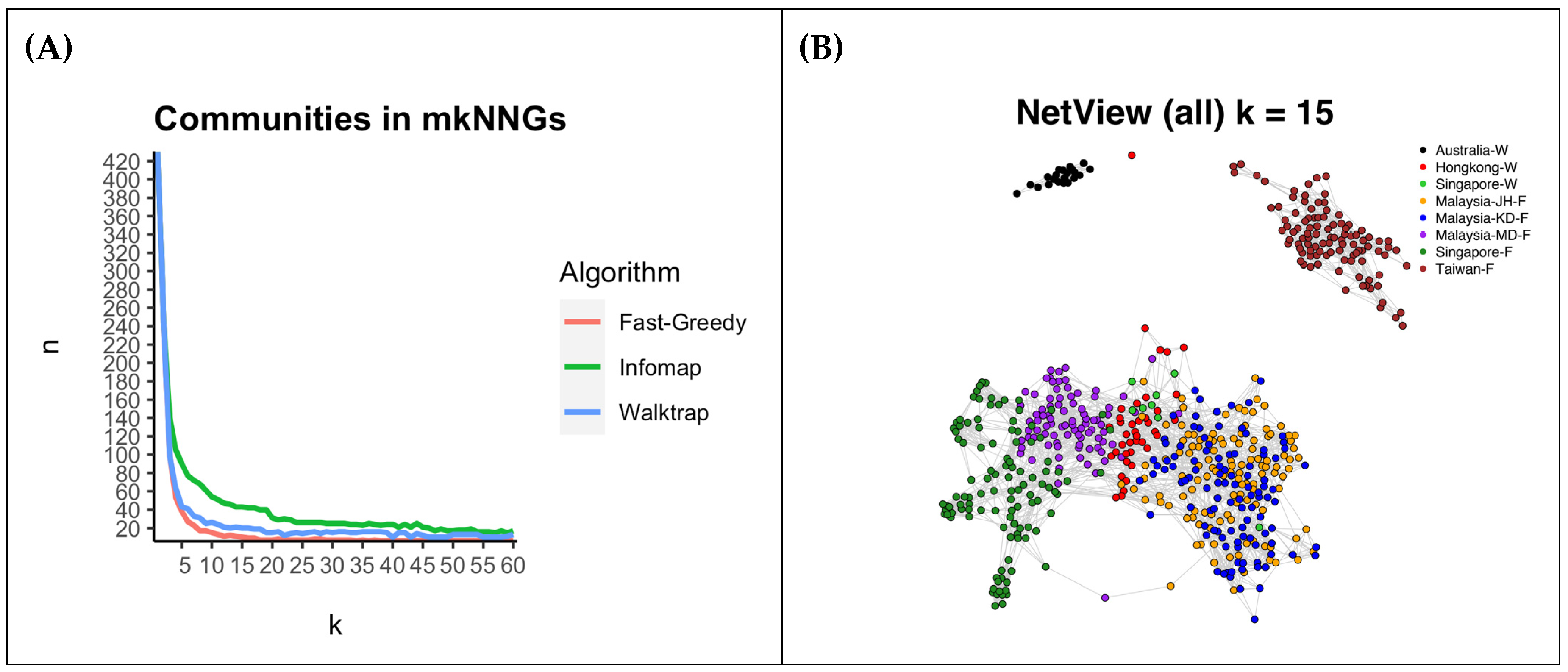
The predicted distribution in wild and sampling localities of our study is presented in Supplementary Figure S1. As seen in Figure 1, a well-defined population clustering was seen, and the network remained split into two connected components at k = 12 to k = 17, indicating strong genetic differentiation of all samples. In the combined analysis, these splits corresponded to the clear separation of the Australian and Taiwanese populations from the remaining populations. At k = 15 (Figure 1B), the NetView k-nearest-neighbor network revealed clear population structure among wild and farm samples. The Australia wild individuals formed a distinct and isolated cluster, while the Taiwan farm population also formed a separate and well-defined component, indicating strong genetic differentiation from the Malaysia–Singapore cluster. Within the South China Sea group, Malaysian farms formed a broadly connected cluster, with Johor, Kedah, and Mixed Malaysia samples interspersed but showing some local grouping, while Singapore (farm) samples clustered more tightly and were positioned adjacent to the Malaysian cluster (Figure 1 and Supplementary Figure S4). Wild populations from Hong Kong and Singapore were embedded at the periphery of this regional cluster, showing close genetic similarity with the Malaysia–Singapore farm populations (Figure 1 and Supplementary Figure S5). Overall, these patterns are consistent with substantial shared ancestry among Malaysia–Singapore farms and a distinct genetic background for the Taiwan group, and strong genetic divergence of the Australia wild population from all other populations.

Furthermore, we performed within-farm relatedness assessment estimated using KING-robust kinship which showed no pairs exceeding the commonly used second-degree threshold (kinship > 0.177) in any farm (proportion = 0 in all farms) (Supplementary Table S2), although a small number of pairs approached the threshold 0.177 (max values ranging 0.1682 to 0.1767).

To zoom in on within-farm relatedness, we generated a relatedness heatmap for these farms using the IBD method, which indicated there are remaining small, related groups of samples despite the cutoff at 0.177 (Supplementary Figure S2), consistent with KING-robust relatedness summaries.

3.4. Genetic Diversity Among Wild-Derived Population

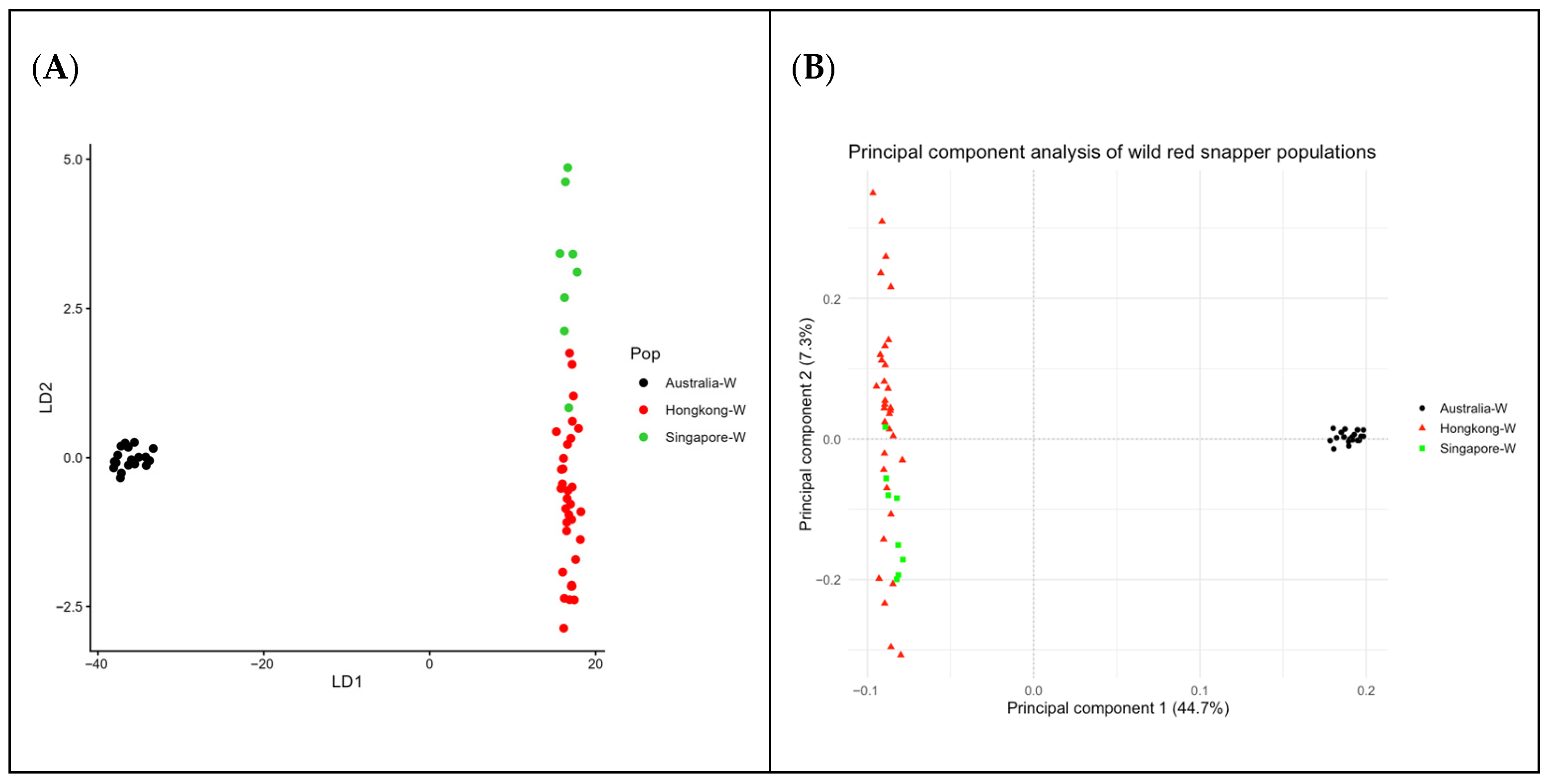
Pairwise F_ST indicated strong differentiation between Australia and both Hong Kong and Singapore (F_ST = 0.200–0.230), whereas differentiation between Hong Kong and Singapore was weak (F_ST = 0.015,

Table 6. Pairwise Weir and Cockerham’s FST estimates among wild populations based on genome-wide SNPs.

Population	Hong Kong	Singapore
Australia	0.200	0.230
Hong Kong		0.015

). Consistent with these estimates, DAPC separated Australia clearly along LD1, while Hong Kong and Singapore showed distinct but with some overlapping samples along LD2 (Figure 2A). Principal component analysis (PCA) further supported this pattern, showing clear separation of the Australia wild population from the other groups along PC1 (44.7% of variance explained), while Hong Kong and Singapore clustered closely together with partial overlap along PC2 (7.3%), indicating weaker differentiation between these two populations relative to the divergence observed for Australia (Figure 2B). Hierarchical AMOVA revealed strong genetic structuring among wild populations, with 47.1% of molecular variance attributable to differences among populations and 52.9% within populations (

Table 7. Analysis of molecular variance (AMOVA) based on permutation testing (p < 0.001, 999 permutations).

AMOVA	SSD	MSD	Df	%
Population	0.734	0.368	2	47.11
Error	1.273	0.022	57	52.88
Total	2.010	0.034	59	100

).

These results consistently indicate strong divergence of the Australia population and comparatively weak differentiation between Hong Kong and Singapore.

3.5. Genetic Connectivity Between Farm and Wild Populations

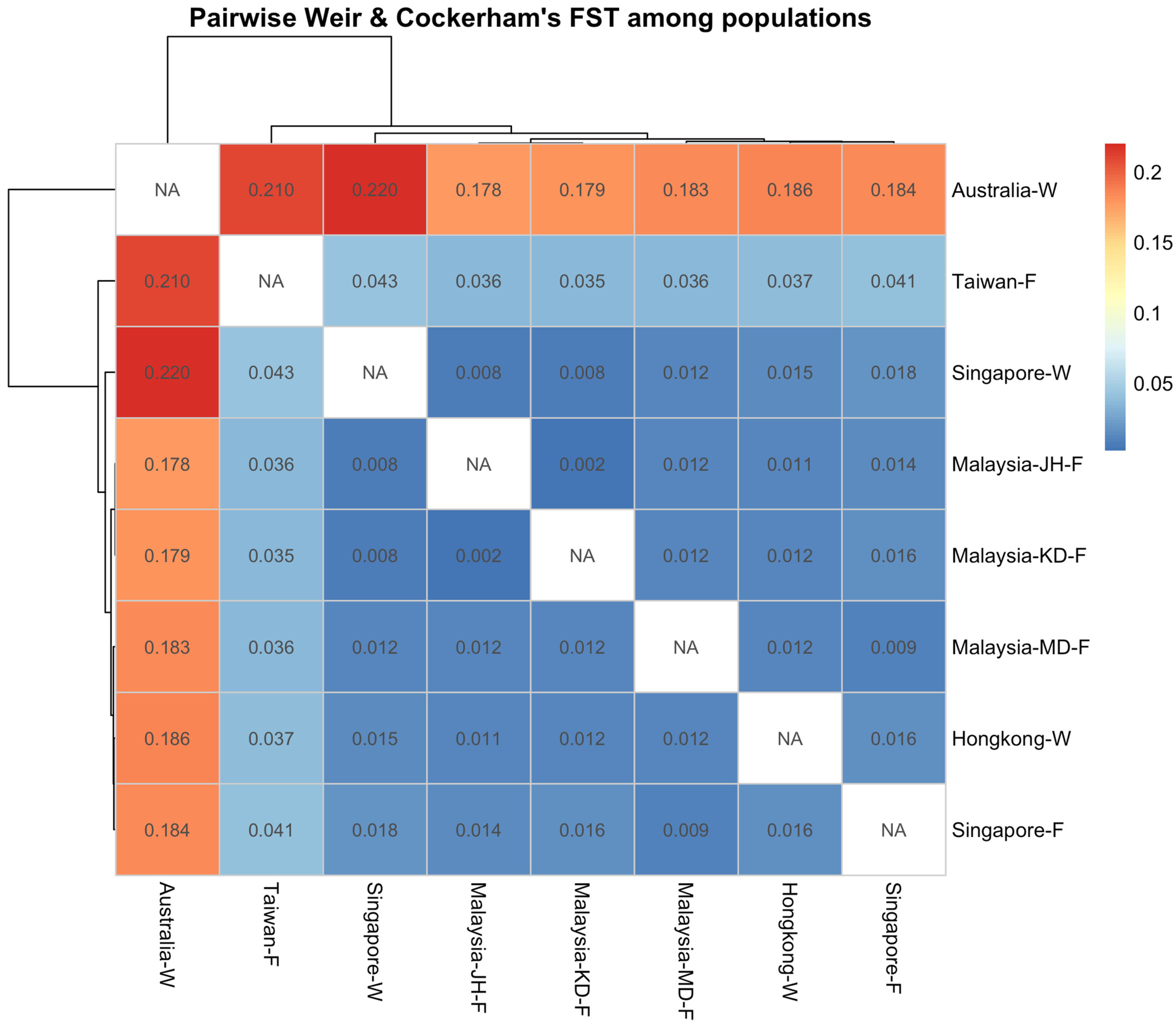
Pairwise FST estimates revealed pronounced differentiation among wild populations and between wild and farm groups (e.g., Australia vs. others F_ST = 0.178–0.220, Figure 3). In contrast, farm populations from Malaysia and Singapore showed consistently low differentiation (F_ST = 0.002–0.016), with Johor and Kedah being nearly indistinguishable (F_ST = 0.002) indicating strong connectivity or shared broodstock sources. Taiwan farms were more differentiated from the Malaysia/Singapore farm cluster (F_ST = 0.035–0.041). Hong Kong-W and Singapore-W showed low differentiation from the Malaysia/Singapore farm populations (FST = 0.008–0.018), suggesting close genetic affinity within the South China Sea group. Bootstrap confidence intervals were narrow and all pairwise comparisons were significant (p < 0.05, Supplementary Table S4).

The population-level FST further supports these patterns (Figure 3). Australia-W formed the most divergent group, Taiwain-F showed moderate genetic differentiation from the Malaysia/Singapore cluster, and the Malaysia/Singapore clustered closely together. Heatmaps of each farm population within individuals are presented in Supplementary Figure S2.

Hierarchical AMOVA partitioned genetic variance among origin (wild vs. farm), among populations nested within origin, and within populations. A small but significant component of variance was attributable to origin (3.14%, p = 0.015), whereas differentiation among populations within origin explained a larger fraction (8.17%, p < 0.001). Most variation occurred within populations (88.69%).

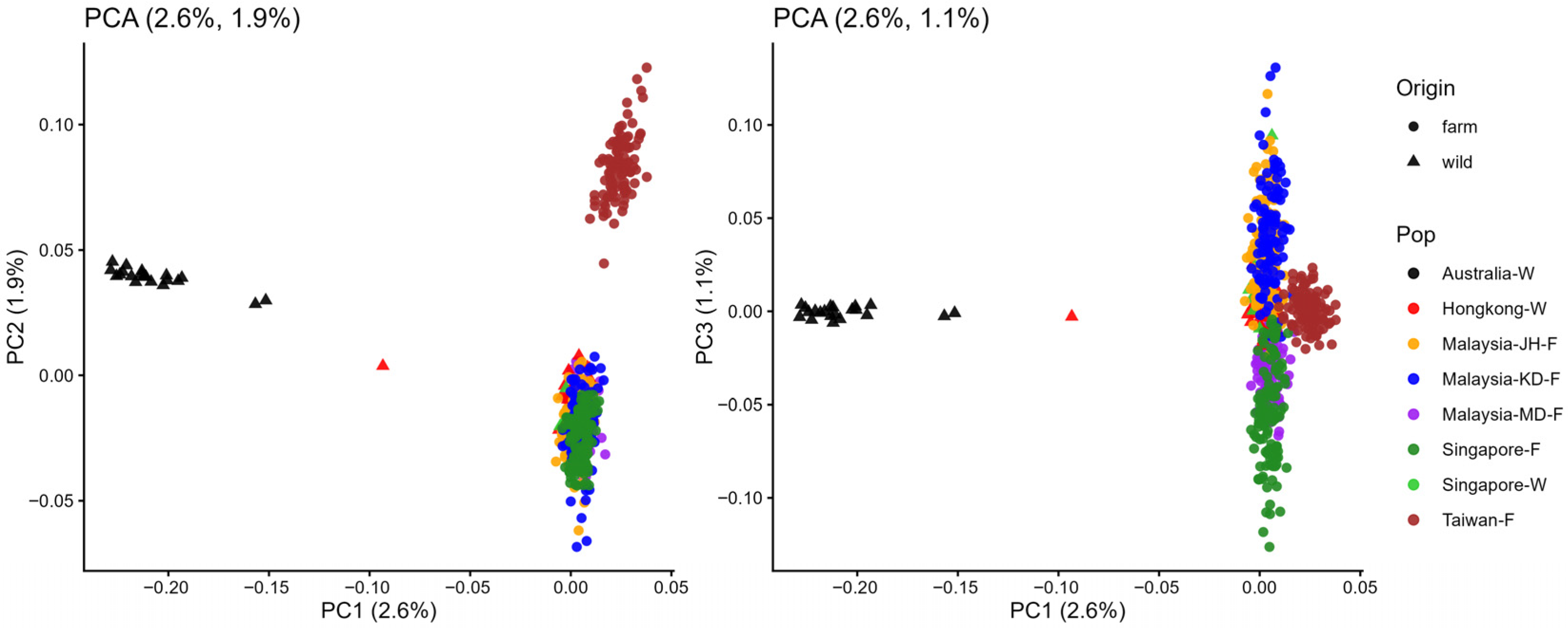
Further analysis was conducted using all populations excluding Australia, as the Australian population showed substantially higher genetic divergence compared to the others. Isolation-by-distance analysis based on a Mantel test revealed a moderate positive correlation between genetic and geographic distances (r = 0.489); however, this relationship was not statistically significant (p = 0.109). This non-significant relationship suggests that geographic distance alone does not explain the observed genetic differentiation among South China Sea populations. Analysis of molecular variance (AMOVA) revealed that the majority of genetic variation was distributed within individuals (95.72%), while only a small proportion was attributed to differences among populations (2.01%). Despite the low magnitude, this component was statistically significant (p = 0.001), indicating weak but detectable genetic differentiation among populations. Variation among individuals within populations also accounted for a small but significant proportion (2.27%, p = 0.003). These results are consistent with ADMIXTURE results (Supplementary Figure S3) and provided additional insight into individual ancestry and population assignment. Cross-validation supported low values of K (K = 2–3) as the most informative representation of population structure. At K = 2, ADMIXTURE identified a primary genetic division separating the Taiwan farm population from all other populations, consistent with its distinct clustering observed in PCA (Figure 4) and NetView analyses. At K = 3, additional structure emerged, with partial differentiation of the Singapore farm population from the broader Malaysia–Singapore cluster, indicating a subtle substructure likely driven by founder effects or breeding practices. Across these K values, Malaysian farm populations (Johor, Kedah, Mixed) and Singapore wild populations showed highly admixed ancestry profiles, supporting substantial genetic connectivity within the South China Sea region. At higher K values (K ≥ 4), inferred clusters became increasingly fragmented and less biologically interpretable, reflecting within-population variation rather than well-defined population structures.

3.6. Farm Assignment Rate

Using assignPOP with 5-fold cross-validation, assignment accuracy differed markedly among farm populations (

Table 8. Assignment rates of five farms using 5-fold cross-validation.

Fold	Training Loci	Johor	Kedah	Mixed	Singapore	Taiwan
		N = 118	N = 106	N = 87	N = 111	N = 102
K = 5	0.1	0.71 ± 0.10	0.56 ± 0.15	0.85 ± 0.11	0.91 ± 0.06	1.00 ± 0.00
K = 5	0.25	0.79 ± 0.11	0.57 ± 0.13	0.91 ± 0.06	0.95 ± 0.03	1.00 ± 0.00
K = 5	0.5	0.70 ± 0.04	0.18 ± 0.13	0.13 ± 0.05	0.62 ± 0.20	1.00 ± 0.00
K = 5	1	0.72 ± 0.07	0.11 ± 0.10	0.19 ± 0.13	0.62 ± 0.13	1.00 ± 0.00

). Taiwan individuals were assigned with perfect accuracy across all locus sampling proportions (1.00 ± 0.00), indicating strong differentiation from other farm groups. Singapore showed consistently high assignment accuracy when using 10–25% of loci (0.91–0.95), while Johor exhibited moderate accuracy (0.70–0.79). In contrast, Kedah and the Mixed group showed reduced and less stable assignment performance, consistent with shared ancestry and/or admixture among Malaysian farm populations. Overall, misclassification patterns suggest substantial genetic connectivity among regional farm sources (Malaysia and Singapore), whereas Taiwan represents a distinct genetic source.

4. Discussion

Using genome-wide SNP data, this study evaluated the population structure, genetic diversity, and connectivity of Lutjanus malabaricus across wild populations from Australia, Hong Kong, and Singapore, and hatchery stocks from Malaysia, Singapore, and Taiwan. The results revealed clear regional genetic structuring, with the Australian wild population strongly differentiated from South China Sea populations. In contrast, farm populations from Malaysia and Singapore showed high genetic connectivity, while the Taiwan farm population formed a distinct cluster. These findings provide a genomic baseline for understanding population connectivity and highlight important considerations for broodstock management and selective breeding of Malabar red snapper across the region.

4.1. Data Quality and Sampling Considerations

The multi-step SNP filtering approach produced high-quality genotype panels suitable for population genomic analyses. Removal of closely related individuals helped minimize biases associated with family structure, which can artificially inflate signals of differentiation in hatchery populations where non-random mating and mass spawning are common. Although some wild populations had relatively small sample sizes, particularly the Singapore wild group, the diversity estimates were consistent with those reported for other marine teleost species with large census sizes [43]. This suggests that the retained SNP datasets captured informative genome-wide variation for assessing population structure and genetic diversity.

4.2. Effective Population Size and Implications for Broodstock Management

LD-based estimates revealed strong contrasts among populations. The Australia wild population showed high Ne (996.2), indicating demographic stability, and making it a valuable source of broodstock. In contrast, Singapore and Taiwan farm populations exhibited Ne values near 50, a level associated with increased inbreeding risk over successive generations [44]. Although F_IS was not elevated, the small Ne suggests limited effective breeders and/or skewed family contributions under mass spawning. For these populations, management should prioritize increasing the effective number of breeders, balancing family contributions, and avoiding repeated use of the same parents [45]. Malaysian farm populations showed moderate Ne (>100), suggesting lower short-term risk. However, without structured mating and genomic monitoring, Ne may decline in closed breeding systems. Regular genomic assessment of relatedness and controlled mating designs are therefore recommended across all hatchery populations to sustain genetic diversity and long-term breeding potential [46].

4.3. Population Differentiation, Connectivity, and Regional Structure

Genome-wide SNP analyses revealed clear geographic structuring of Lutjanus malabaricus across the study region. The strongest pattern was the pronounced differentiation of the Australian wild population from all South China Sea populations. Similar population subdivision has previously been reported in Indo-Pacific snappers and other reef-associated fishes, with limited connectivity between northern Australian and Southeast Asian populations [13,14,47]. Such divergence is consistent with major biogeographic barriers across the Indo-Malay Archipelago that restrict larval dispersal and gene flow among marine populations [48,49,50]. These findings suggest that Australian populations likely represent a distinct regional genetic unit and should therefore be considered separately in fisheries management and broodstock sourcing strategies.

Within the South China Sea region, genetic differentiation among populations was generally low, indicating substantial regional connectivity. Farm populations from Malaysia and Singapore showed very weak differentiation and strong clustering, suggesting shared broodstock origins or historical exchange of seed among hatcheries, a pattern commonly observed in aquaculture systems where broodstock or juveniles are frequently transferred among facilities [51,52]. In contrast, the Taiwan farm population formed a distinct cluster relative to the Malaysia–Singapore group, likely reflecting a different broodstock origin or founder effects during hatchery establishment. Wild populations from Hong Kong and Singapore clustered closely with the Malaysia–Singapore farm populations, suggesting that hatchery stocks may have originated from regional wild sources or from a shared broodstock pool. The absence of significant isolation-by-distance after excluding the divergent Australian population indicates that geographic separation is not the primary driver of genetic differentiation among the studied populations. This pattern is consistent with aquaculture systems, where broodstock movement, translocation, and shared hatchery sources can disrupt natural spatial genetic structure. As a result, populations from different geographic locations may remain genetically similar despite large distances.

From a management perspective, the low differentiation observed among Malaysia and Singapore hatcheries suggests that broodstock exchange within this regional cluster is unlikely to introduce major genetic discontinuities. However, the strong divergence of the Australian and Taiwan populations indicates that movement of broodstock across these regions should be approached cautiously. The strong differentiation observed between Australian and Southeast Asian populations may partly reflect isolation-by-distance processes associated with large geographic separation. Limited larval dispersal across major biogeographic barriers, combined with large spatial distances between northern Australia and the South China Sea region, may reduce gene flow and promote regional genetic divergence.

Mixing highly differentiated populations may disrupt locally adapted genetic backgrounds or influence breeding outcomes, particularly if hatchery escapees interact with wild stocks [18,53]. Interpretation of connectivity patterns among farm populations should also consider the limited availability of detailed broodstock sourcing records. In many Southeast Asian aquaculture systems, broodstock exchange among hatcheries and sourcing from local fisheries are common practices. Such regional exchange of genetic material may contribute to the relatively low genetic differentiation observed among Malaysia and Singapore farm populations.

4.4. Assignment Patterns Highlight Hatchery Connectivity

Assignment testing using assignPOP restricted to farm populations addressed a practical management question: whether individuals show strong genetic ‘signatures’ of their recorded farm or whether frequent misclassification indicates shared ancestry/mixing among hatcheries. Using 5-fold cross-validation, assignment performance differed markedly among farms. Taiwan showed consistently high assignment accuracy (often near perfect), consistent with its distinct position in F_ST/PCA. Singapore generally assigned well at lower proportions of loci, while Johor was moderate. In contrast, Kedah and Mixed showed lower and less stable assignment rates, consistent with greater genetic similarity to other Malaysian farms and/or higher admixture among those populations. These misclassification patterns align with the very low pairwise differentiation among Malaysian farms and support the interpretation of a connected regional hatchery gene pool across Malaysia and Singapore, rather than strongly isolated farm lineages. Historical sourcing of eggs/fry across Malaysia and Taiwan for Singapore aquaculture provides a plausible mechanism for these patterns, although direct inference of directionality or timing of transfers is not possible from assignment alone [54]. From a management perspective, high hatchery connectivity can be beneficial if it maintains diversity, but it can also obscure provenance and reduce traceability of broodstock origins. Conversely, the strong separation of Australia wild and Taiwan farm suggests caution with inter-regional broodstock movement, as mixing strongly divergent sources may alter locally adapted genetic backgrounds and create unpredictable outcomes in breeding programs.

4.5. Implications for Aquaculture and Broodstock Management

The genomic patterns identified in this study have direct implications for aquaculture development and broodstock management of Lutjanus malabaricus. The strong genetic connectivity observed among Malaysia and Singapore farm populations suggests that regional broodstock exchange can be implemented with minimal risk of genetic incompatibility, provided that biosecurity and traceability are maintained. However, the low effective population sizes observed in Singapore and Taiwan farms highlight an urgent need for improved broodstock management strategies, including increasing the number of breeding individuals, balancing family contributions, and implementing genomic-based mating designs to limit inbreeding accumulation.

In contrast, the pronounced genetic differentiation of the Australian wild population indicates that it should be managed as a separate genetic resource, and translocation of broodstock between Australia and Southeast Asia should be approached cautiously to avoid disrupting locally adapted gene pools. Overall, integrating genomic monitoring into breeding programs will be essential to maintain genetic diversity, improve selection response, and ensure long-term sustainability of red snapper aquaculture in the region.

Interactions between farmed and wild populations represent an important consideration for the long-term sustainability of red snapper aquaculture. Expansion of marine cage culture increases the likelihood of escape events, which may facilitate genetic introgression between cultured stocks and wild populations. Although relatively low genetic differentiation was observed between several farm and nearby wild populations in the South China Sea region, this pattern may reflect shared broodstock origins rather than ongoing natural gene flow. If farm-derived individuals escape and interbreed with wild populations, repeated introgression could alter allele frequencies and potentially reduce local adaptation over time, particularly if hatchery stocks originate from geographically distant sources. Such genetic risks have been widely documented in other aquaculture species, particularly Atlantic salmon, where escapees have contributed to measurable changes in wild population structure. While similar large-scale impacts have not yet been widely reported for Lutjanus malabaricus, the observed connectivity among Southeast Asian farm populations highlights the importance of implementing traceability systems, improving containment strategies, and conducting routine genetic monitoring of cultured stocks.

4.6. Implications for Selective Breeding and Future Work

The genomic dataset generated in this study, particularly from farmed populations, provides a valuable foundation for modeling and optimizing selective breeding strategies for Malabar red snapper. The availability of high-quality SNP panels allows accurate parameterization of stochastic simulation tools such as AlphaSimR [55], QMSim [56], or MoBPS [57]. These simulations can incorporate realistic starting genetic diversity, inbreeding levels, and migration patterns observed here, enabling predictions of long-term genetic gain, inbreeding accumulation, and allele frequency dynamics under different selection intensities and mating designs. Such genomic tools will be particularly valuable for emerging breeding programs in Southeast Asia, where domestication of this species remains relatively recent.

Farm-specific Ne estimates highlight populations (e.g., Singapore, Taiwan) where diversity conservation should be prioritized in breeding program designs. By integrating genomic relationships and trait-specific heritabilities from ongoing or future phenotyping, simulation outputs can guide optimal broodstock replacement rates, cross-population introgression scenarios, and strategies for balancing short-term gains with long-term genetic health [58,59]. This approach will bridge the gap between the current genetic baseline and targeted improvements in growth, feed efficiency, and disease resistance for sustainable aquaculture production, especially for Singaporean farms.

5. Conclusions

This study provides a foundational understanding of the genetic structure and diversity of Lutjanus malabaricus across northern Australia and the South China Sea. The pronounced genetic isolation of the Australian population highlights the need for tailored management, while wild and farmed populations within the South China Sea share comparable diversity. However, the marked decline in effective population sizes in Singaporean and Taiwanese farms underscores the urgency of implementing genetic monitoring and improved broodstock management to mitigate inbreeding risks and ensure long-term sustainability. This emphasizes the importance of collaborative management to safeguard shared genetic resources. By establishing a regional baseline of population genetics, this study supports the development of selective breeding programs and demonstrates the value of molecular tools in promoting sustainable aquaculture and fisheries management. Collectively, these findings provide a practical genomic framework to guide broodstock management and selective breeding strategies for sustainable aquaculture of Lutjanus malabaricus.

References

1. Thevasagayam, N.M.; Sridatta, P.S.; Jiang, J.; Tong, A.; Saju, J.M.; Kathiresan, P.; Kwan, H.Y.; Ngoh, S.Y.; Liew, W.C.; Kuznetsova, I.S.; et al. Transcriptome survey of a marine food fish: Asian seabass (Lates calcarifer). J. Mar. Sci. Eng. 2015, 3, 382–400. [Google Scholar] [CrossRef] [Scilit]
2. Kiron, V.; Kathiresan, P.; Fernandes, J.M.O.; Sørensen, M.; Vasanth, G.K.; Lin, Q.; Lin, Q.; Lim, T.K.; Dahle, D.; Dias, J.; et al. Clues from the intestinal mucus proteome of Atlantic salmon to counter inflammation. J. Proteom. 2022, 255, 104487. [Google Scholar] [CrossRef] [Scilit] [PubMed]
3. Verdegem, M.; Buschmann, A.H.; Latt, U.W.; Dalsgaard, A.J.T.; Lovatelli, A. The contribution of aquaculture systems to global aquaculture production. J. World Aquac. Soc. 2023, 54, 206–250. [Google Scholar] [CrossRef] [Scilit]
4. Purushothaman, K.; Vu, N.T.; Loh, J.-Y.; Liang, B.; Domingos, J.A.; Vij, S. Stability of muscle fatty acids and proximate composition across phenotypic traits in Malabar red snapper (Lutjanus malabaricus). J. Food Compos. Anal. 2026, 153, 109133. [Google Scholar] [CrossRef] [Scilit]
5. Muldoon, G.; Peterson, L.; Johnston, B. Economic and market analysis of the live reef food fish trade in the Asia-Pacific region. SPC Live Reef Fish Inf. Bull. 2005, 13, 35–41. [Google Scholar]
6. FAO. FishStatJ—Software for Fishery and Aquaculture Statistical Time Series; FAO: Rome, Italy, 2022; Volume 2022. [Google Scholar]
7. Purushothaman, K.; Vu, N.T.; Qing, S.D.T.R.; Koh, J.; Mohamed, M.H.B.; Wen, R.H.J.; Liang, B.; Loo, G.; Domingos, J.A.; Jerry, D.R.; et al. Genetic evaluation of nutritional traits in Malabar red snapper (Lutjanus malabaricus): Heritability and genetic correlations of fatty acid composition. Aquaculture 2025, 599, 742144. [Google Scholar] [CrossRef] [Scilit]
8. Liang, B.; Jerry, D.R.; Nguyen, V.; Shen, X.; Koh, J.; Terence, C.; Nayfa, M.G.; Carrai, M.; Kathiresan, P.; Ho, R.J.W.; et al. Genetic parameters and genotype by environment interaction for harvest traits of Malabar red snapper (Lutjanus malabaricus). Aquaculture 2025, 600, 742247. [Google Scholar] [CrossRef] [Scilit]
9. Dinh, Y.H.T.; Lam, N.H.; Lishchenko, F.V. Life-history traits variation of Lutjanus malabaricus (Bloch & Schneider, 1801) in the waters off Northern Vietnam. J. Mar. Biol. Assoc. UK 2023, 103, e45. [Google Scholar] [CrossRef] [Scilit]
10. Herwaty, S.; Mallawa, A.; Najamuddin, N.; Zainuddin, M. Age, growth, mortality, and population characteristics of the red snapper (Lutjanus malabaricus) in the Timor Sea waters, Indonesia. Biodiversitas J. Biol. Divers. 2023, 24, 2217–2224. [Google Scholar] [CrossRef] [Scilit]
11. Kathiresan, P.; Vu, N.T.; Liang, B.; Qing, S.D.T.R.; bin Mohamed, M.H.; Wen, R.H.J.; Shen, X.; Jones, D.B.; Loo, G.; Jerry, D.R.; et al. Investigating genomic prediction accuracies for muscle fatty acids composition in Malabar red snapper (Lutjanus malabaricus). Aquaculture 2025, 613, 743398. [Google Scholar] [CrossRef] [Scilit]
12. Purushothaman, K.; Wen, R.H.J.; bin Mohamed, M.H.; Qing, S.D.T.R.; Wuan, L.H.; Liang, B.; Vu, N.T.; Voigtmann, M.; Press, C.M.; Loo, G.; et al. Comparative Nutritional and Histological Analysis of Malabar Red Snapper (Lutjanus malabaricus) and Asian Seabass (Lates calcarifer). Animals 2024, 14, 1803. [Google Scholar] [CrossRef] [Scilit] [PubMed]
13. Blaber, S.J.M.; Dichmont, C.M.; Buckworth, R.C.; Badrudin; Sumiono, B.; Nurhakim, S.; Iskandar, B.; Fegan, B.; Ramm, D.C.; Salini, J.P. Shared Stocks of Snappers (Lutjanidae) in Australia and Indonesia: Integrating Biology, Population Dynamics and Socio-Economics toExamine Management Scenarios. Rev. Fish Biol. Fish. 2005, 15, 111–127. [Google Scholar] [CrossRef] [Scilit]
14. Salini, J.P.; Ovenden, J.R.; Street, R.; Pendrey, R.; Haryanti; Ngurah. Genetic population structure of red snappers (Lutjanus malabaricus Bloch & Schneider, 1801 and Lutjanus erythropterus Bloch, 1790) in central and eastern Indonesia and northern Australia. J. Fish Biol. 2006, 68, 217–234. [Google Scholar] [CrossRef] [Scilit]
15. Fry, G.; Milton, D.A.; Van Der Velde, T.; Stobutzki, I.; Andamari, R.; Badrudin; Sumiono, B. Reproductive dynamics and nursery habitat preferences of two commercially important Indo-Pacific red snappers Lutjanus erythropterus and L. malabaricus. Fish. Sci. 2009, 75, 145–158. [Google Scholar] [CrossRef] [Scilit]
16. Zhang, J.; Cai, Z.; Huang, L. Population genetic structure of crimson snapper Lutjanus erythropterus in East Asia, revealed by analysis of the mitochondrial control region. ICES J. Mar. Sci. 2006, 63, 693–704. [Google Scholar] [CrossRef] [Scilit]
17. Tave, D. Inbreeding and Brood Stock Management; Food & Agriculture Org.: Rome, Italy, 1999. [Google Scholar]
18. Jensen, Ø.; Dempster, T.; Thorstad, E.B.; Uglem, I.; Fredheim, A. Escapes of fishes from Norwegian sea-cage aquaculture: Causes, consequences and prevention. Aquac. Environ. Interact. 2010, 1, 71–83. [Google Scholar] [CrossRef] [Scilit]
19. Aguirre, N.C.; Filippi, C.V.; Zaina, G.; Rivas, J.G.; Acuña, C.V.; Villalba, P.V.; García, M.N.; González, S.; Rivarola, M.; Martínez, M.C.; et al. Optimizing ddRADseq in Non-Model Species: A Case Study in Eucalyptus dunnii Maiden. Agronomy 2019, 9, 484. [Google Scholar] [CrossRef] [Scilit]
20. Lavretsky, P.; DaCosta, J.M.; Sorenson, M.D.; McCracken, K.G.; Peters, J.L. ddRAD-seq data reveal significant genome-wide population structure and divergent genomic regions that distinguish the mallard and close relatives in North America. Mol. Ecol. 2019, 28, 2594–2609. [Google Scholar] [CrossRef] [Scilit] [PubMed]
21. Dodds, K.G.; McEwan, J.C.; Brauning, R.; Anderson, R.M.; van Stijn, T.C.; Kristjánsson, T.; Clarke, S.M. Construction of relatedness matrices using genotyping-by-sequencing data. BMC Genom. 2015, 16, 1047. [Google Scholar] [CrossRef] [Scilit]
22. Anderson, C.B.; Franzmayr, B.K.; Hong, S.W.; Larking, A.C.; van Stijn, T.C.; Tan, R.; Moraga, R.; Faville, M.J.; Griffiths, A.G. Protocol: A versatile, inexpensive, high-throughput plant genomic DNA extraction method suitable for genotyping-by-sequencing. Plant Methods 2018, 14, 75. [Google Scholar] [CrossRef] [Scilit]
23. Elshire, R.J.; Glaubitz, J.C.; Sun, Q.; Poland, J.A.; Kawamoto, K.; Buckler, E.S.; Mitchell, S.E. A Robust, Simple Genotyping-by-Sequencing (GBS) Approach for High Diversity Species. PLoS ONE 2011, 6, e19379. [Google Scholar] [CrossRef] [Scilit] [PubMed]
24. Catchen, J.M.; Amores, A.; Hohenlohe, P.; Cresko, W.; Postlethwait, J.H. Stacks: Building and Genotyping Loci De Novo from Short-Read Sequences. G3 Genes Genomes Genet. 2011, 1, 171–182. [Google Scholar] [CrossRef] [Scilit]
25. Li, H. Aligning sequence reads, clone sequences and assembly contigs with BWA-MEM. arXiv 2013, arXiv:1303.3997. [Google Scholar] [CrossRef] [Scilit]
26. Li, H.; Handsaker, B.; Wysoker, A.; Fennell, T.; Ruan, J.; Homer, N.; Marth, G.; Abecasis, G.; Durbin, R.; Subgroup, G.P.D.P. The sequence alignment/map format and SAMtools. Bioinformatics 2009, 25, 2078–2079. [Google Scholar] [CrossRef] [Scilit]
27. Danecek, P.; Bonfield, J.K.; Liddle, J.; Marshall, J.; Ohan, V.; Pollard, M.O.; Whitwham, A.; Keane, T.; McCarthy, S.A.; Davies, R.M.; et al. Twelve years of SAMtools and BCFtools. GigaScience 2021, 10, giab008. [Google Scholar] [CrossRef] [Scilit]
28. Purcell, S.; Neale, B.; Todd-Brown, K.; Thomas, L.; Ferreira, M.A.R.; Bender, D.; Maller, J.; Sklar, P.; de Bakker, P.I.W.; Daly, M.J.; et al. PLINK: A Tool Set for Whole-Genome Association and Population-Based Linkage Analyses. Am. J. Hum. Genet. 2007, 81, 559–575. [Google Scholar] [CrossRef] [Scilit]
29. Chang, C.C.; Chow, C.C.; Tellier, L.C.; Vattikuti, S.; Purcell, S.M.; Lee, J.J. Second-generation PLINK: Rising to the challenge of larger and richer datasets. Gigascience 2015, 4, 7. [Google Scholar] [CrossRef] [Scilit]
30. Keenan, K.; Mcginnity, P.; Cross, T.; Crozier, W.; Prodöhl, P. diveRsity: An R package for the estimation and exploration of population genetics parameters and their associated errors. Methods Ecol. Evol. 2013, 4, 782–788. [Google Scholar] [CrossRef] [Scilit]
31. Do, C.; Waples, R.S.; Peel, D.; Macbeth, G.; Tillett, B.J.; Ovenden, J.R. NeEstimator v2: Re-implementation of software for the estimation of contemporary effective population size (Ne) from genetic data. Mol. Ecol. Resour. 2014, 14, 209–214. [Google Scholar] [CrossRef] [Scilit] [PubMed]
32. Pembleton, L.W.; Cogan, N.O.I.; Forster, J.W. StAMPP: An R package for calculation of genetic differentiation and structure of mixed-ploidy level populations. Mol. Ecol. Resour. 2013, 13, 946–952. [Google Scholar] [CrossRef] [Scilit] [PubMed]
33. Steinig, E.J.; Neuditschko, M.; Khatkar, M.S.; Raadsma, H.W.; Zenger, K.R. netview p: A network visualization tool to unravel complex population structure using genome-wide SNP s. Mol. Ecol. Resour. 2016, 16, 216–227. [Google Scholar] [CrossRef] [Scilit] [PubMed]
34. Neuditschko, M.; Khatkar, M.S.; Raadsma, H.W. NetView: A High-Definition Network-Visualization Approach to Detect Fine-Scale Population Structures from Genome-Wide Patterns of Variation. PLoS ONE 2012, 7, e48375. [Google Scholar] [CrossRef] [Scilit]
35. Zheng, X.; Levine, D.; Shen, J.; Gogarten, S.M.; Laurie, C.; Weir, B.S. A high-performance computing toolset for relatedness and principal component analysis of SNP data. Bioinformatics 2012, 28, 3326–3328. [Google Scholar] [CrossRef] [Scilit] [PubMed]
36. Weir, B.S.; Cockerham, C.C. Estimating F-statistics for the analysis of population structure. Evolution 1984, 38, 1358–1370. [Google Scholar] [CrossRef] [Scilit] [PubMed]
37. Paradis, E. pegas: An R package for population genetics with an integrated–modular approach. Bioinformatics 2010, 26, 419–420. [Google Scholar] [CrossRef] [Scilit]
38. Jombart, T. adegenet: A R package for the multivariate analysis of genetic markers. Bioinformatics 2008, 24, 1403–1405. [Google Scholar] [CrossRef] [Scilit]
39. Alexander, D.H.; Novembre, J.; Lange, K. Fast model-based estimation of ancestry in unrelated individuals. Genome Res. 2009, 19, 1655–1664. [Google Scholar] [CrossRef] [Scilit]
40. Kamvar, Z.N.; Tabima, J.F.; Grünwald, N.J. Poppr: An R package for genetic analysis of populations with clonal or partially clonal reproduction. PeerJ 2014, 2014, e281. [Google Scholar] [CrossRef] [Scilit]
41. Oksanen, J.; Blanchet, F.G.; Kindt, R.; Legendre, P.; Minchin, P.R.; O’hara, R.; Simpson, G.L.; Solymos, P.; Stevens, M.H.H.; Wagner, H. Package ‘vegan’. Community Ecol. Package Version 2013, 2, 1–295. [Google Scholar]
42. Chen, K.-Y.; Marschall, E.A.; Sovic, M.G.; Fries, A.C.; Gibbs, H.L.; Ludsin, S.A. assignPOP: An r package for population assignment using genetic, non-genetic, or integrated data in a machine-learning framework. Methods Ecol. Evol. 2018, 9, 439–446. [Google Scholar] [CrossRef] [Scilit]
43. Liu, B.L.; Chen, X.J.; Chen, Y.; Hu, G.Y. Determination of squid age using upper beak rostrum sections: Technique improvement and comparison with the statolith. Mar. Biol. 2015, 162, 1685–1693. [Google Scholar] [CrossRef] [Scilit]
44. Frankham, R.; Bradshaw, C.J.A.; Brook, B.W. Genetics in conservation management: Revised recommendations for the 50/500 rules, Red List criteria and population viability analyses. Biol. Conserv. 2014, 170, 56–63. [Google Scholar] [CrossRef] [Scilit]
45. Sonesson, A.K.; Hallerman, E.; Humphries, F.; Hilsdorf, A.W.S.; Leskien, D.; Rosendal, K.; Bartley, D.; Hu, X.; Garcia Gomez, R.; Mair, G.C. Sustainable management and improvement of genetic resources for aquaculture. J. World Aquac. Soc. 2023, 54, 364–396. [Google Scholar] [CrossRef] [Scilit]
46. Bentsen, H.B.; Olesen, I. Designing aquaculture mass selection programs to avoid high inbreeding rates. Aquaculture 2002, 204, 349–359. [Google Scholar] [CrossRef] [Scilit]
47. Ovenden, J.R.; Berry, O.; Welch, D.J.; Buckworth, R.C.; Dichmont, C.M. Ocean’s eleven: A critical evaluation of the role of population, evolutionary and molecular genetics in the management of wild fisheries. Fish Fish. 2013, 16, 125–159. [Google Scholar] [CrossRef] [Scilit]
48. Lohman, D.J.; de Bruyn, M.; Page, T.; von Rintelen, K.; Hall, R.; Ng, P.K.; Shih, H.-T.; Carvalho, G.R.; von Rintelen, T. Biogeography of the Indo-Australian Archipelago. Annu. Rev. Ecol. Evol. Syst. 2011, 42, 205–226. [Google Scholar] [CrossRef] [Scilit]
49. Carpenter, K.E.; Barber, P.H.; Crandall, E.D.; Ablan-Lagman, M.C.A.; Ambariyanto; Mahardika, G.N.; Manjaji-Matsumoto, B.M.; Juinio-Meñez, M.A.; Santos, M.D.; Starger, C.J.; et al. Comparative Phylogeography of the Coral Triangle and Implications for Marine Management. J. Mar. Biol. 2010, 2011, 396982. [Google Scholar] [CrossRef] [Scilit]
50. Gaither, M.R.; Toonen, R.J.; Robertson, D.R.; Planes, S.; Bowen, B.W. Genetic evaluation of marine biogeographical barriers: Perspectives from two widespread Indo-Pacific snappers (Lutjanus kasmira and Lutjanus fulvus). J. Biogeogr. 2009, 37, 133–147. [Google Scholar] [CrossRef] [Scilit]
51. Gjedrem, T.; Baranski, M. Selective Breeding in Aquaculture: An Introduction; Springer Nature: Durham, NC, USA, 2009; ISBN 9789048127726. [Google Scholar]
52. Lind, C.; Ponzoni, R.; Nguyen, N.; Khaw, H. Selective Breeding in Fish and Conservation of Genetic Resources for Aquaculture. Reprod. Domest. Anim. 2012, 47, 255–263. [Google Scholar] [CrossRef] [Scilit]
53. Laikre, L.; Schwartz, M.K.; Waples, R.S.; Ryman, N. Compromising genetic diversity in the wild: Unmonitored large-scale release of plants and animals. Trends Ecol. Evol. 2010, 25, 520–529. [Google Scholar] [CrossRef] [Scilit]
54. Shen, Y.; Ma, K.; Yue, G.H. Status, challenges and trends of aquaculture in Singapore. Aquaculture 2021, 533, 736210. [Google Scholar] [CrossRef] [Scilit]
55. Gaynor, R.C.; Gorjanc, G.; Hickey, J.M. AlphaSimR: An R package for breeding program simulations. G3 Genes Genomes Genet. 2021, 11, jkaa017. [Google Scholar] [CrossRef] [Scilit]
56. Sargolzaei, M.; Schenkel, F.S. QMSim: A large-scale genome simulator for livestock. Bioinformatics 2009, 25, 680–681. [Google Scholar] [CrossRef] [Scilit]
57. Pook, T.; Schlather, M.; Simianer, H. MoBPS-modular breeding program simulator. G3 Genes Genomes Genet. 2020, 10, 1915–1918. [Google Scholar] [CrossRef] [Scilit]
58. Berg, P.; Nielsen, J.; Sørensen, M. EVA: Realized and predicted optimal genetic contributions. In Proceedings of the 8th World Congress on Genetics Applied to Livestock Production, Belo Horizonte, Minas Gerais, Brazil, 13–18 August 2006. [Google Scholar]
59. Wellmann, R. Optimum contribution selection for animal breeding and conservation: The R package optiSel. BMC Bioinform. 2019, 20, 25. [Google Scholar] [CrossRef] [Scilit]
Figure 1. NetView analysis of farm samples. (A) Number of communities across k (Fast-Greedy, Infomap, Walktrap), showing a plateau around k = 12–17. (B) kNN network at k = 15, with nodes colored by population and edges representing IBS-based nearest-neighbor connections.
Aquacj 06 00017 g001
Figure 2. (A) Discriminant analysis of principal components (DAPC) showing strong separation of Australia from the other populations along LD1, while Hong Kong and Singapore cluster closely with near separation. FST uncertainty was assessed by locus bootstrapping (1000 replicates; 95% CI). Permutation-based p-values were <0.001 for all comparisons but should be interpreted cautiously for groups with small sample size such as Singapore (n = 8). (B) Principal component analysis (PCA) across wild populations.
Aquacj 06 00017 g002
Figure 3. Pairwise genetic differentiation among wild and farm-derived Malabar red snapper populations. Heatmap shows Weir and Cockerham’s FST estimates among eight populations. Higher values indicate stronger genetic differentiation. Australia wild showed the greatest differentiation from all South China Sea populations, whereas Malaysia and Singapore farm populations showed low differentiation, consistent with high genetic connectivity. Taiwan farm was moderately differentiated from the Malaysia–Singapore cluster.
Aquacj 06 00017 g003
Figure 4. Principal component analysis of wild and farm-derived Malabar red snapper populations. (Left) PCA based on PC1 (2.6%) and PC2 (1.9%) showing strong separation of the Australia wild population and clear differentiation of the Taiwan farm population from the Malaysia–Singapore cluster. (Right) PCA based on PC1 (2.6%) and PC3 (1.1%) providing additional resolution of finer-scale structure within the South China Sea populations, highlighting subtle differentiation among farm populations while maintaining substantial overlap among Malaysia and Singapore groups.
Aquacj 06 00017 g004