Comparative Time-Series Modeling and Forecasting of Tilapia Broodfish Growth in Pond and Recirculating Aquaculture Systems (RAS) Using ARIMA

Abstract

This study applied time-series modeling using autoregressive integrated moving average (ARIMA) to compare the growth performance of tilapia broodfish in pond and recirculating aquaculture systems (RAS) from June 2023 to May 2024. Descriptive statistics showed a higher mean percentage weight gain under RAS (26.69%) than pond culture (23.75%), although monthly variability in the RAS dataset was influenced by an outlier, which may be attributed to influential exogenous factors rather than water-quality parameters. Normality, stationarity, and autocorrelation diagnostics confirmed that both datasets were appropriate for ARIMA modeling without differencing. Multiple ARIMA models were evaluated based on RMSE, MAPE, MAE, AIC, BIC, and residual behavior; ARIMA (1,0,1) emerged as the best fit for both systems. Forecasting up to May 2028 revealed stable long-term growth patterns, with RAS consistently showing slightly higher forecasted growth compared to pond culture, although the difference remained small in absolute terms. Predictions remained within model-generated 95% confidence intervals; however, these results indicate internal model consistency rather than independent validation of predictive accuracy. The findings highlight that RAS offers more consistent and slightly superior growth performance, supporting its potential for optimized broodfish production. Recommendations emphasize adopting RAS for enhanced growth predictability and improved management in tilapia aquaculture.

1. Introduction

Aquaculture is now a core pillar of global food systems as fisheries capture has leveled off and demand has continued to rise. “Blue foods” research has highlighted that aquatic foods can generate outsized benefits for nutrition, livelihoods, and climate mitigation when expansion is guided by context-specific governance and technology choices [1,2,3,4,5]. In this landscape, Nile tilapia (Oreochromis niloticus) has become one of the world’s most widely cultivated finfish because it grows rapidly, tolerates a wide range of environmental conditions, and supports diverse production models from extensive ponds to highly intensive indoor systems [6,7,8,9]. Yet, as production intensifies, operational risks associated with climate variability, water-quality instability, and biological uncertainty increasingly shape profitability and sustainability outcomes, particularly in tropical and subtropical regions [10,11,12,13,14].

Bangladesh illustrates both the promise and fragility of rapid freshwater aquaculture growth. Pond-based farming remains dominant, supported by an expanding hatchery and nursery sector, but farms and hatcheries face rising exposure to heat stress, irregular rainfall, and seasonal transitions that destabilize dissolved oxygen, pH, and nitrogen dynamics. These shifts can affect broodstock conditioning, spawning synchrony, larval survival, and seed quality, ultimately constraining consistent production [15,16]. Empirical time-series work has further shown that climatic covariates and pond water-quality parameters can jointly shape tilapia broodfish growth trajectories, implying that growth variability is not simply “noise” but a structured signal that can be modeled to improve decision-making [15,17,18].

Recirculating aquaculture systems (RAS) are increasingly promoted as a climate-adaptation strategy because they operate in controlled environments, reuse water efficiently, and can enhance biosecurity by reducing exposure to external pollutants and pathogens [10,19,20]. In principle, RAS can stabilize temperature and dissolved oxygen and limit ammonia accumulation, thereby reducing environmental stress and improving fish growth. Comparative evidence in tropical contexts also suggests that controlled systems may deliver more consistent seed performance than open ponds under variable climatic and water-quality conditions [21]. However, these benefits come with trade-offs, including higher capital requirements, greater operational complexity, and potentially substantial energy demand, all of which influence adoption and the net environmental footprint of intensification pathways [10].

As production systems diversify, forecasting has emerged as a practical “control layer” for modern aquaculture, supporting proactive feeding and aeration, harvest scheduling, staffing and input procurement, and early warning when growth trajectories diverge from expectations. Forecasting is already widely used in other sectors with seasonal and noisy data streams, and competition-style evaluations have reinforced the importance of transparent benchmarking against strong statistical baselines [22,23]. In aquaculture, this matters because many farm datasets are short, irregular, and subject to structural breaks caused by disease events, management changes, or extreme weather. Under these conditions, parsimonious models such as ARIMA often remain competitive due to their interpretability, diagnostic tooling, and ability to quantify uncertainty [24], while exogenous-variable variants (e.g., ARIMAX) can incorporate environmental drivers when reliable covariates exist [15].

While numerous studies have compared the growth performance of tilapia between pond culture and recirculating aquaculture systems, most assessments rely primarily on descriptive statistics or short-term experimental observations. Consequently, relatively little attention has been given to how growth signals behave over time and how forecasting models can support proactive aquaculture management. Applying ARIMA-based time-series forecasting allows routine growth observations to be transformed into predictive information that can assist with management decisions such as feed planning, broodstock conditioning, production scheduling, and early detection of abnormal growth trends. By comparing forecasting behavior between pond and RAS environments, this study not only evaluates biological performance but also examines how culture system design influences the predictability and temporal dynamics of broodfish growth.

Despite growing interest in data-driven aquaculture, a persistent gap remains, and we still lack clear comparative evidence on how forecasting performance and model assumptions differ between open pond environments and controlled RAS settings for the same species and management objective. Ponds are shaped by exogenous climate forcing and biogeochemical feedback that can create non-stationarity and regime shifts, whereas RAS dynamics may be more stable but can include abrupt operational interventions (e.g., biofilter maintenance, partial water exchange, disinfection cycles) that also introduce discontinuities. Bridging this gap is essential for translating modeling advances into actionable management tools, especially for broodstock programs where growth and condition affect seed output and downstream farm productivity [16,25,26]. Although descriptive statistics can compare average growth performance between pond and RAS, they do not capture the temporal structure of longitudinal growth data. In sequential datasets, observations may exhibit autocorrelation and lag effects that influence future growth patterns. Time-series modeling is therefore necessary to analyze these temporal dependencies and to generate forecasts of future growth based on past observations. In this context, the present study is designed to test the hypothesis that controlled aquaculture environments such as RAS generate more stable and predictable growth trajectories than traditional pond systems. By comparing the time-series characteristics of tilapia broodfish growth in these two production environments, the study evaluates how environmental stability influences growth variability and forecasting reliability.

Therefore, the present study aims to evaluate the internal predictive performance of these models. Specifically, the objectives of this study are to: (i) compare the growth performance of tilapia broodfish in pond and RAS environments; (ii) develop and validate ARIMA-based forecasting models to predict future growth trends in both pond and RAS; and (iii) evaluate the predictive reliability of these models to support improved broodstock management and production planning under variable environmental conditions.

To achieve these objectives, longitudinal growth data of Nile tilapia broodfish cultured in both pond and RAS were analyzed using time-series modeling techniques. The ARIMA framework was applied following the Box–Jenkins methodology to identify suitable model structures, estimate parameters, and generate forecasts of broodfish growth trends. This comparative modeling approach provides insights into the temporal dynamics of tilapia growth under contrasting production systems and highlights the potential application of forecasting tools for improving broodstock management and production planning in aquaculture.

2. Materials and Methods

2.1. Ethical Statement

The study included fish sampling from ponds and RAS, among other activities. All animal scientific procedures were strictly followed and were conducted with prior approval from the Animal Welfare and Ethics Committee of Bangladesh Agricultural University (BAU) (Ref. no. BAURES/ESRC/FISH-11/2022).

2.2. Study Area

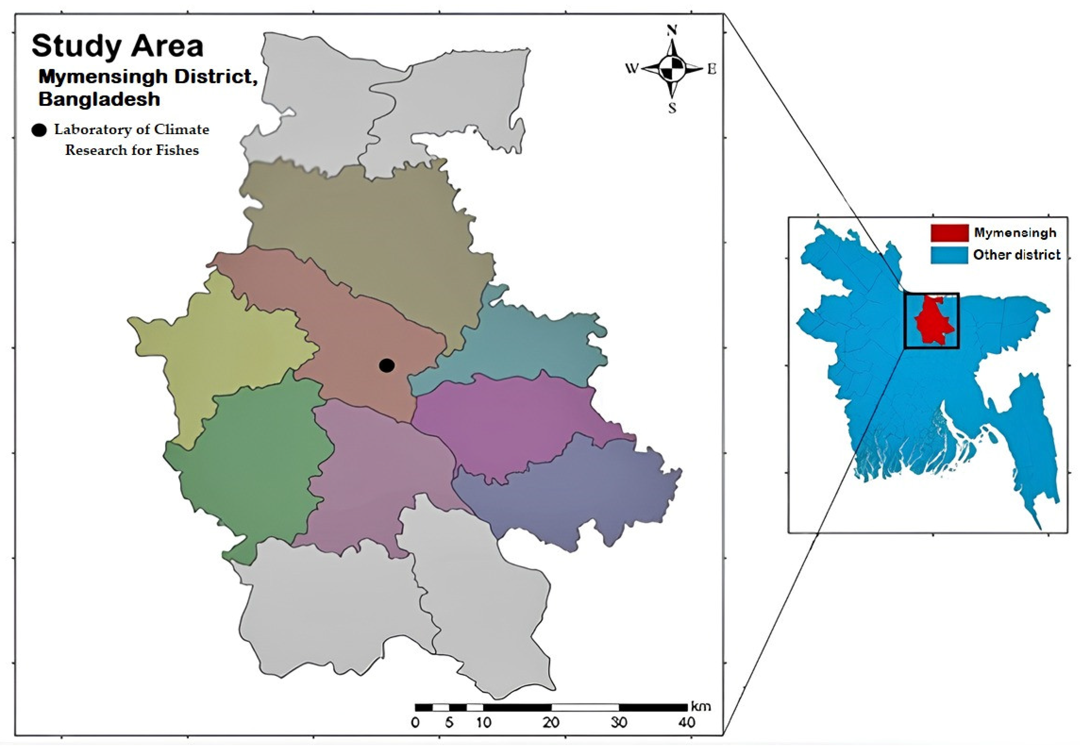
The study was carried out in two separate aquaculture settings: pond-based systems and environment-controlled RAS at the Laboratory of Climate Research for Fishes (LCRF), Bangladesh Agricultural University (BAU), Mymensingh (Figure A1). The LCRF at BAU was selected as the study site because it provides well-equipped laboratory facilities that enable intensive data collection and detailed analysis relevant to this study. The study was conducted from June 2023 to May 2024.

2.3. Collection and Domestication of Broodfish

Three earthen ponds (26 ft × 17 ft × 2.6 ft; area 1149.2 ft³ or 32.54 m³ of each) were used for pond culture. The ponds were dried out completely. The undesired small fish, aquatic weeds, etc., were removed from the ponds. Excess bottom mud was removed and used to repair the broken and uneven dykes. Lime was applied at 1 kg/decimal in the bottom and dyke during pond preparation. After refilling, ponds were left undisturbed for seven days before stocking.

The RAS consisted of three concrete rearing tanks (10,000 L each) and operated as a closed-loop system with 8–10% daily water exchange and complete recirculation approximately every 5 h. Before stocking, all RAS machinery and system components were thoroughly cleaned, operated, and verified to be fully functional. The system included solids removal using a swirl separator and drum filter, mechanical and biological filtration with bio-balls and volcanic rock, protein skimming, degassing, oxygen cone, eco-trap and UV sterilization. Dissolved oxygen was maintained above 6 mg L⁻¹, and water temperature was automatically regulated at 29 ± 0.5 °C [27].

A total of 600 Nile tilapia (Oreochromis niloticus) broodfish (mean length 15.5 ± 1.4 cm; mean weight 60.47 ± 6.14 g) were collected from Asia Scientific Hatchery and Nursery and stocked equally in ponds (300 fish) and RAS (300 fish) with a 40:60 sex ratio after proper acclimation. The selected stocking densities for both pond and RAS were determined based on established broodstock management guidelines and the carrying capacity of the experimental units, ensuring adequate space, stable water quality, and minimizing density-related stress to maintain optimal broodfish growth and reproductive performance. Utilizing commercial floating feed with 35% protein content, the broodfish were fed twice a day at a quantity averaging 2% to 4% of their body weight. Throughout the study period, systematic random sampling was employed to monitor broodstock health, physical attributes, growth trends, disease prevalence, and pond productivity.

2.4. Assessment of Growth of Tilapia Broodfish in Traditional Pond and RAS

The growth performance of tilapia broodfish was evaluated in both traditional pond systems and RAS using replicated experimental units. Randomly selected broodfish from each system were sampled four times per month in the morning (10:00–11:00 AM), with 10 fish (male: female = 1:1) collected per sampling event. After collection, total length (TL, cm) was measured to the nearest 0.1 cm using a measuring scale, and total body weight (TBW, g) was recorded using a digital balance (TANITA KD-160, Max 2 kg, TANITA, Tokyo, Japan). After biometric measurements, all sampled fish were carefully returned to their respective ponds and RAS tanks to maintain stock continuity and minimize disturbance to the experimental population. To ensure consistency between the sampling design and the presentation of results, the growth values reported in this study represent monthly mean values calculated from the four sampling events conducted each month. Mean length and weight of sampled fish from ponds and RAS were recorded throughout the stocking period and at each sampling point to assess growth performance. Growth and feed-utilization parameters were calculated using standard aquaculture Equations (1)–(4):

$$\%Lengthgain={\displaystyle \frac{L_2-L_1}{L_i}}\times 100$$

(1)

$$\%Weightgain={\displaystyle \frac{W_2-W_1}{W_1}}\times 100$$

(2)

$$Foodconversionratio(FCR)={\displaystyle \frac{Totalfeedsupplied\left(\mathrm{g}\right)}{Liveweightgain\left(\mathrm{g}\right)}}$$

(3)

$$SGR(\%/\mathrm{day})={\displaystyle \frac{\mathit{ln}{W}_f-\mathit{ln}{W}_i}{t}}\times 100$$

(4)

where $L_1$ and $L_2$ are the mean initial and final total lengths (cm), $W_1$ and $W_2$ are the mean initial and final live body weights (g) measured at times $T_1$ and $T_2$ (days), respectively, and $\mathrm{l}\mathrm{n}$ denotes the natural logarithm. Live weight gain was computed as $W_2-W_1$.

2.5. Assessment of Water-Quality Parameters in Pond and RAS

Water-quality parameters were monitored in both pond systems and laboratory-controlled RAS at regular intervals. To capture daily fluctuations associated with photosynthesis and climatic variation, measurements were taken twice daily (morning and afternoon). The monitored parameters included water temperature, dissolved oxygen (DO), pH, ammonia, transparency, and total dissolved solids (TDS). Water temperature was measured using a digital thermometer (SMART Sensor AR867, SMART SENSOR, Dongguan, China). Dissolved oxygen (DO) was measured using a portable DO meter (DO-5509, Lutron Electronic Enterprise, Taiwan). pH was measured using a compact digital pH meter (pH-107, Hangzhou, Fuzhou, China). Total dissolved solids (TDS) were measured using a handheld TDS meter (TDS-3, HM Digital, Culver City, CA, USA, manufactured in China). Ammonia concentration was determined using a commercial test kit (Lifesonic Innovations Pvt. Ltd., Raiganj, India).

2.6. Comparative Time-Series Modeling and Forecasting of Tilapia Broodfish Growth in Pond and RAS Using ARIMA

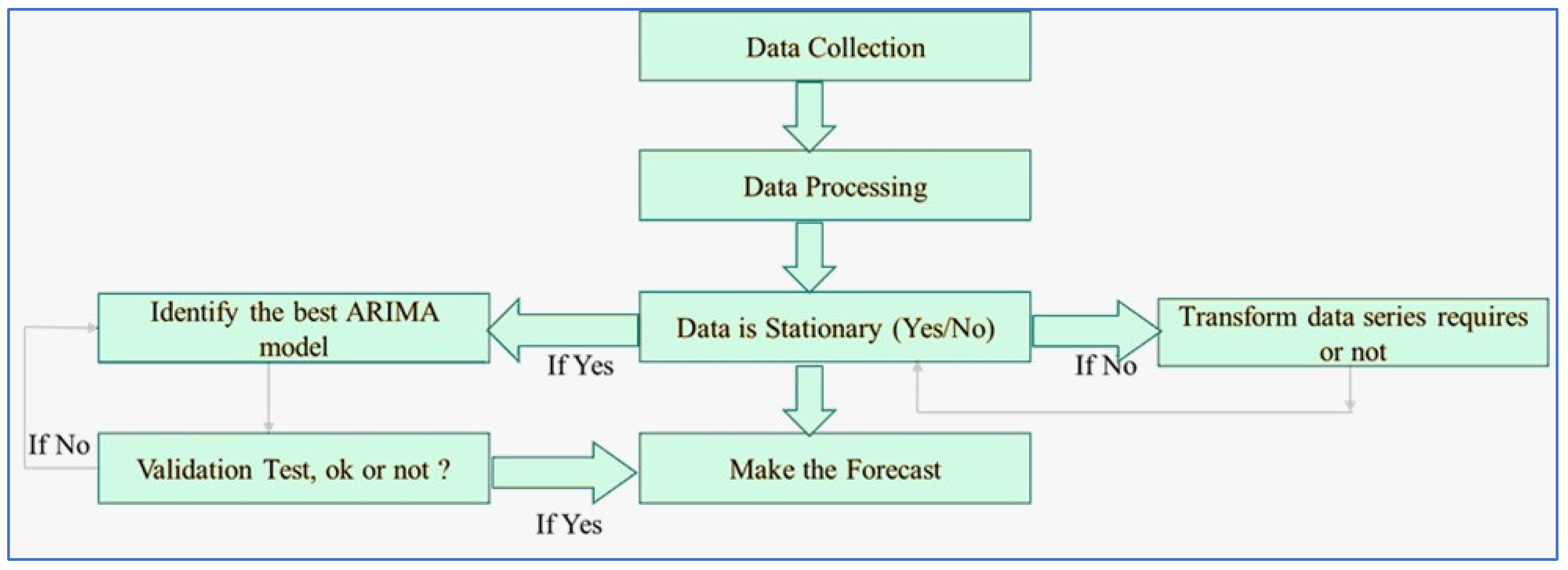
This investigation employed the ARIMA model for projecting future scenarios of broodfish growth trends based on the longitudinal data obtained from traditional pond and RAS. Although fish were sampled four times per month during the study period, resulting in 48 sampling observations, the time-series modeling was performed using monthly mean values derived from these four sampling events. Thus, 12 monthly data points were used as the input series for ARIMA modeling and forecasting. Monthly aggregation was applied to reduce within-month sampling variability and to align the analysis with system-level management cycles; however, this approach reduces the number of observations and may limit statistical power and model sensitivity. Individual fish measurements were used to calculate system-level monthly mean growth values, which served as the time-series input for ARIMA modeling. The time series analyzed in this study represents aggregated monthly system-level growth metrics rather than repeated measurements at the individual fish level. Given the relatively small sample size (n = 12), the time-series analysis should be interpreted as exploratory rather than confirmatory, and the results should be considered indicative rather than definitive. The limited number of observations may reduce the statistical power of model diagnostics such as ACF, PACF, and ADF tests, and may increase uncertainty in long-term forecasts. The ARIMA model comprises three key components: Autoregression (AR), which establishes relationships between current values and past observations; Integration (I), involving differencing to achieve stationarity in non-stationary time series; and Moving Average (MA), which captures patterns from previous forecast errors [28]. The ARIMA modeling framework applied in this study was univariate, meaning that forecasts were generated solely from the historical growth time series. Environmental and climatic variables (e.g., rainfall, temperature, dissolved oxygen, and ammonia) were not included as exogenous predictors in the model. The objective was to evaluate the baseline predictive performance of ARIMA using growth observations alone. This integrated approach is well-suited for dynamic production data with temporal fluctuations, as it effectively captures both short-term fluctuations and long-term underlying patterns. The systematic process of ARIMA model development, encompassing identification, estimation, diagnostic checking, and forecasting, adhered to the established Box–Jenkins methodology (Figure 1) [29].

The modeling followed the Box–Jenkins framework, comprising four key steps: identifying a potential model, estimating parameters, validating assumptions, and generating forecasts. To ensure the data met the stationarity requirements as a prerequisite for ARIMA modeling, we applied the augmented Dickey–Fuller (ADF) test and, where necessary, transformed the data through differencing. Stationarity was assessed using the augmented Dickey–Fuller (ADF) test and visual inspection of time-series behavior. Stationarity is crucial in time-series analysis, as it ensures that the statistical properties of the series, such as mean and variance, remain constant over time [30]. Because the data represent sequential observations over time, temporal autocorrelation is expected and is explicitly modeled within the ARIMA framework. The differencing transformation was not applied as the stationarity condition was satisfied.

2.6.1. Model Identification

The first step in ARIMA modeling involved identifying a suitable model structure. This process was carried out by examining the autocorrelation function (ACF) and partial autocorrelation function (PACF) plots of the time series to determine possible model specifications [31]. The ACF measures the relationship between current observations and their lagged values, whereas the PACF evaluates this relationship after controlling for the effects of intervening lags. Together, these diagnostic tools assist in selecting appropriate orders for the autoregressive (AR) and moving average (MA) components by indicating statistically significant lag patterns. An ARIMA model is typically represented as ARIMA (p, d, q), where p refers to the order of the autoregressive term, d represents the degree of differencing applied to achieve stationarity, and q denotes the order of the moving average term. The autoregressive component, AR(p), describes the dependence of the current observation on its own past values. This relationship is represented in Equation (5) as follows:

X_t = ϕ₁X_t−1 + ϕ₂X_t−2 + … + ϕ_pX_t−p + ε_t

(5)

In this equation, X_t represents the observed value at time t, ϵ_t is the white-noise error term at time t, and ϕ₁, ϕ₂,…,ϕ_p are the autoregressive parameters to be estimated.

Conversely, the moving average component, MA(q), captures the dependence of the current observation on past error terms (residuals) from previous time steps, as represented in Equation (6):

X_t = μ + ε_t + θ₁ε_t−1 + θ₂ε_t−2 + …+ θ_qε_t−q

(6)

Here, X_t represents the observed value at time t, μ denotes the mean of the time series, ε_t is the white-noise error term at time t, and θ₁, θ₂, …, θ_q are the parameters that need to be estimated. The integration order, d, specifies the number of differencing steps required to achieve stationarity, a critical step for stabilizing the mean by eliminating trends and seasonal patterns.

After identifying models through ACF and PACF diagnostics, parameter estimation was conducted to determine the most suitable values of p, d, and q. The resulting alternative models were assessed and compared using the Bayesian information criterion (BIC), where lower BIC values indicated a more favorable balance between goodness of fit and model parsimony.

The selected model was subsequently subjected to residual diagnostics to verify that the residuals followed a normal distribution with a mean of zero and exhibited constant variance. This diagnostic evaluation confirmed that the ARIMA model adequately captured the underlying structure of the time series, thereby ensuring its robustness and reliability for forecasting tilapia growth trends in both traditional pond systems and RAS.

2.6.2. Estimation of Parameters

The second stage of the ARIMA modeling framework focused on estimating the parameters of the previously identified models. Parameter optimization was carried out using nonlinear least squares and maximum likelihood estimation (MLE) techniques [32]. Among these approaches, nonlinear least squares are widely applied for estimating ARIMA parameters, as demonstrated in earlier studies [33].

To assess the reliability of the estimated parameters and the overall performance of the models, several evaluation criteria were employed, including root mean square error (RMSE), mean absolute percentage error (MAPE), maximum absolute percentage error (MaxAPE), mean absolute error (MAE), maximum absolute error (MaxAE), Akaike information criterion (AIC), and Bayesian information criterion (BIC). These statistical measures enabled a comprehensive evaluation of model fit and forecasting accuracy. Models yielding lower error and information criteria (AIC and BIC) were considered preferable; however, model selection also emphasized parsimony to avoid overfitting, particularly given the limited sample size [34]. The mathematical formulations of RMSE, MAPE, MaxAPE, MAE, MaxAE, and BIC are presented in Equations (7)–(13), respectively.

$$\mathrm{R}\mathrm{M}\mathrm{S}\mathrm{E}=\sqrt{{\displaystyle \frac{1}{n}}{\sum }_{t=1}^n{e}_t^2},$$

(7)

where e_t = A_t − F_t, the residual or error at time t (i.e., difference between the actual value A_t and the forecasted value F_t), n: total number of observations.

$$\mathrm{MAPE}={\displaystyle \frac{100\%}{n}}{\sum }_{t=1}^n\left|{\displaystyle \frac{e_t}{y_t}}\right|$$

(8)

where e_t = A_t − F_t, the residual or error at time t (the difference between the actual value A_t and the forecasted value F_t), y_t: the actual value at time t, n: the total number of observations.

$$\mathrm{M}\mathrm{a}\mathrm{x}\mathrm{A}\mathrm{P}\mathrm{E}=\mathrm{m}\mathrm{a}\mathrm{x}\left(\left|{\displaystyle \frac{A_t-F_t}{A_t}}\right|\times 100\right)$$

(9)

where A_t represents the actual value at time t. F_t refers to the forecasted or predicted value at time t.

$$\mathrm{M}\mathrm{A}\mathrm{E}=\frac{1}{n}{\sum }_{t=1}^n\left|{\displaystyle e_t}\right|$$

(10)

where e_t = A_t − F_t, the residual or error at time t (the difference between the actual value A_t and the forecasted value F_t), n: the total number of observations.

$$\mathrm{M}\mathrm{a}\mathrm{x}\mathrm{A}\mathrm{E}=\max \left(\left|A_t-F_t\right|\right)$$

(11)

where A_t is the actual value at time t. F_t is the forecasted or predicted value at time t.

The standard formula for Akaike information criterion (AIC) is:

$$\mathrm{A}\mathrm{I}\mathrm{C}=-2\mathrm{l}\mathrm{n}\left(\mathrm{L}\right)+2\mathrm{k}$$

(12)

where

L = maximum likelihood of the model, k = number of estimated parameters in the model, and ln = natural logarithm

BIC was considered in 1978 as

BIC = T′log(σ²) + (p + q + 1)logT′

(13)

Here, σ² indicates the mean square error and T′ indicates the number of observations used. The model with the lowest BIC value will be the best [35].

2.6.3. Diagnostic Test of Residuals

The third stage of ARIMA modeling involved a comprehensive diagnostic evaluation of the model residuals. ACF and PACF plots of the residuals were analyzed to verify whether they behaved as white-noise, indicating that the fitted model had adequately captured the underlying structure of the time series. In cases where residuals deviated from white noise behavior, additional diagnostic procedures were applied to examine their randomness and conformity to a normal distribution. This verification ensured that the estimated ARIMA model appropriately represented the observed data.

To further assess residual normality, both normal probability plots and histograms of the residuals were visually examined. Residuals closely following a straight line in the normal probability plot indicated an approximately normal distribution, while a symmetric, bell-shaped histogram further supported this assumption. These graphical diagnostics were essential for validating the normality requirement of the model residuals and provided intuitive insights into their distributional properties. Ultimately, the optimal ARIMA model was selected based on the minimization of multiple evaluation criteria, including RMSE, MAPE, MaxAPE, MAE, MaxAE, and BIC, with the final choice guided by the specific objectives of the analysis.

2.6.4. Forecasting

The final stage of the ARIMA modeling process focused on producing forecasts of tilapia growth for both traditional pond systems and RAS. The forecasting performance of the selected model was assessed in comparison with alternative specifications using established evaluation metrics, including RMSE, MAPE, MaxAPE, MAE, MaxAE, and the BIC. In addition, forecast confidence intervals were generated to define the range within which future observations are likely to occur, thereby accounting for uncertainty associated with the predictions [34]. Within an ARIMA (p, d, q) framework, future values of the series are modeled as a linear function of past observations and historical error terms, as represented in Equation (14).

Δ^d + Y_t = ∅₀ + Δ^dY_t = ∅₀ + ∅₁Δ^dY_t−1 + ∅₂Δ^dY_t−2 + …… + ∅_pΔ^dY_t−p + ε_t + θ₁ ε_t−1 + θ₂ε_t−2 + …… + θ_q ε_t−q

(14)

where Y_t signifies the actual value and ϵ_t represents the random error at time t. The parameter d indicates the number of differencing transformations required to achieve time-series stationarity. ϕ_i and θ_j are the autoregressive and moving average coefficients, respectively, while p and q are integers denoting the orders of these components. The autoregressive terms account for the influence of past observations, while the moving-average terms capture the impact of previous forecast errors. These components, along with the constant term (ϕ0), collectively define the ARIMA model for time-series analysis.

2.7. Statistical Analysis

Data entry, compilation, and structural organization were carried out using Microsoft Excel 2016, while descriptive statistical analyses and exploratory visualizations, including moving averages and seasonal decomposition, were performed in Minitab 2019. Time-series modeling and forecasting were implemented in RStudio (R version 4.5.2) following the Box–Jenkins methodological framework. This procedure comprised data preprocessing and stationarity evaluation using the ADF test, with differencing applied where necessary, followed by model identification through ACF and PACF analyses, parameter estimation, and diagnostic validation.

Residual diagnostics included visual assessments of normal probability plots and histograms to confirm normality assumptions. Model selection was guided by the minimization of error and information criteria, namely RMSE, MAPE, MAE, MaxAE, MaxAPE, and BIC. In cases where multiple models exhibited comparable performance, the principle of parsimony and evidence of residual whiteness, assessed through residual ACF and PACF plots, were used to determine the most appropriate model. Forecast confidence intervals were generated at the 95% level to account for predictive uncertainty. Additionally, independent sample t-tests were conducted to compare growth performance parameters between pond and RAS, and the corresponding p-values were calculated to determine statistical significance. Overall, the analysis followed a sequential workflow encompassing data preprocessing, model fitting, performance evaluation, and post-analysis validation.

3. Results

3.1. Comparative Growth Performance of Tilapia Broodfish in Pond and RAS

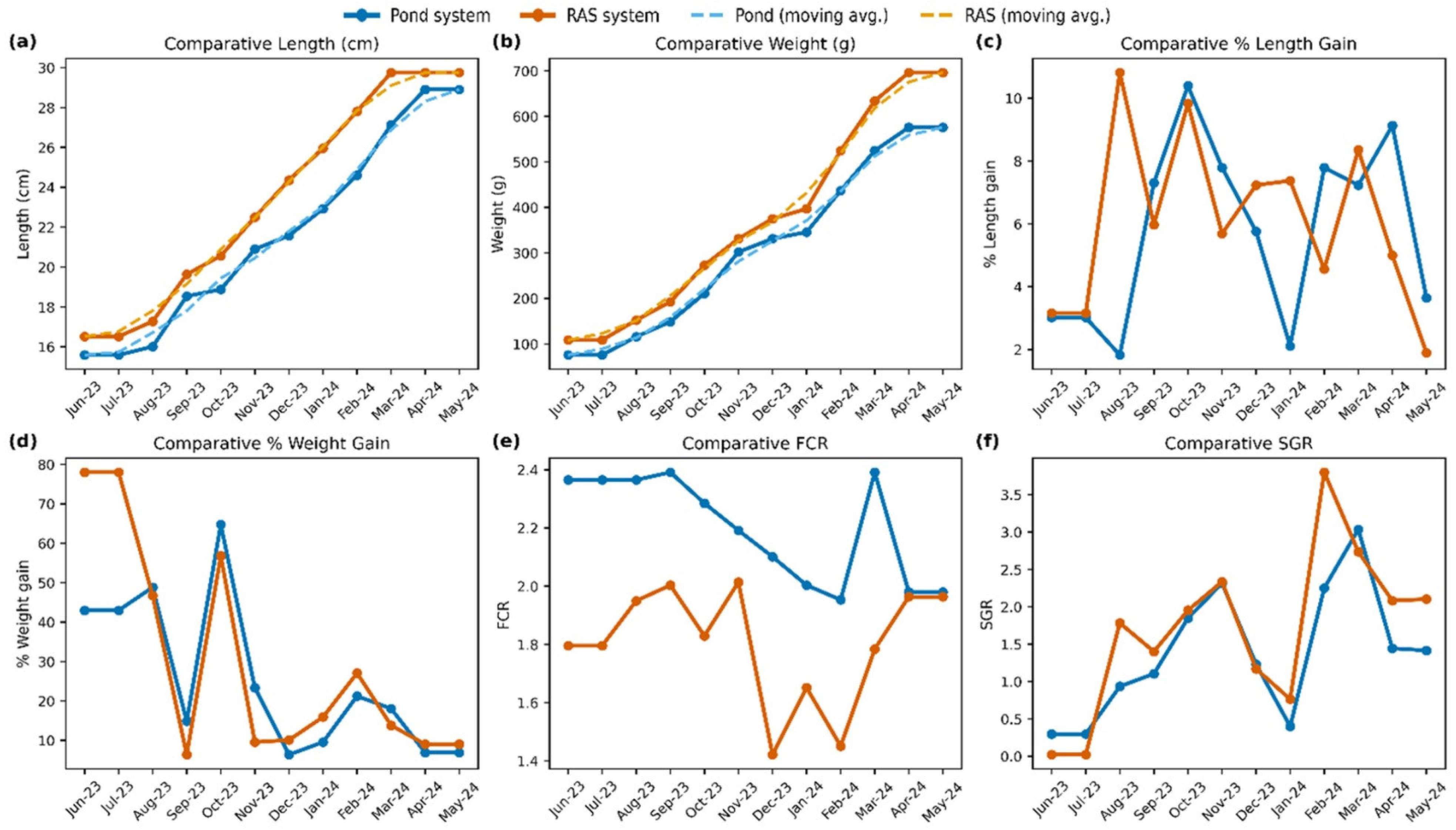
Tilapia broodfish reared in the recirculating aquaculture system (RAS) showed consistently better growth and performance than fish cultured in traditional ponds. Both groups began with identical mean initial length (15.5 ± 1.4 cm) and mean initial weight (60.47 ± 6.14 g), supporting a fair comparison between systems (

Table 1. Growth performance parameters with mean values (± SD) in the pond and RAS with statistical comparison using an independent sample t-test.

Parameters	Pond (Mean ± SD)	RAS (Mean ± SD)	p-Value
Mean Initial Length (cm)	15.5 ± 1.4	15.5 ± 1.4	1.000
Mean Final Length (cm)	26.96 ± 4.57	28.63 ± 2.69	0.621
Mean Initial Weight (g)	60.47 ± 6.14	60.47 ± 6.14	1.000
Mean final Weight (g)	540.57 ± 10.62	658.40 ± 20.15	0.0028
Total Weight Gain (g)	480.05 ± 45.08	597.93 ± 40.24	0.0284
Total Length Gain (cm)	11.39 ± 0.34	13.13 ± 0.53	0.0129
Specific Growth Rate (SGR) (%Day−1)	0.66 ± 08	0.72 ± 0.05	0.343
Feed Conversion Ratio (FCR)	2.21 ± 0.37	1.75 ± 0.09	0.158
Survival Rate (%)	89.33%	96.67%	0.0002

Note: p-values were calculated using independent sample t-tests to compare growth performance parameters between pond and RAS.

). By the end of the culture period, broodfish in RAS attained a higher mean final length (28.63 ± 2.69 cm) than pond-reared fish (26.96 ± 4.57 cm) (Table 1 and Figure 2a). Mean final weight followed the same pattern, with RAS fish reaching 658.40 ± 20.15 g compared with 540.57 ± 10.62 g in ponds (Table 1 and Figure 2b).

Growth increments were also greater under RAS conditions. Total weight gain was 597.93 ± 40.24 g in RAS, while pond fish gained 480.05 ± 45.08 g (Table 1). Total length gain was similarly higher in RAS (13.13 ± 0.53 cm) than in ponds (11.39 ± 0.34 cm) (Table 1). When expressed as proportional change, RAS fish showed higher percentage length gain and percentage weight gain (Figure 2c,d). Feed-utilization efficiency differed markedly between systems: the feed conversion ratio (FCR) was lower in RAS (1.75 ± 0.09) than in ponds (2.21 ± 0.37), indicating more efficient feed conversion in the recirculating environment (Table 1 and Figure 2e). The specific growth rate (SGR) was slightly higher in RAS (0.72 ± 0.05% day⁻¹) compared with ponds (0.66 ± 0.08% day⁻¹), reflecting improved daily growth performance (Table 1 and Figure 2f). Survival was also higher in RAS (96.67%) than in pond culture (89.33%) (Table 1). Overall, across all indicators (length, weight, gains, FCR, SGR and survival), RAS outperformed pond culture (Table 1 and Figure 2). Statistical comparison using independent sample t-tests indicated that final weight, total weight gain, total length gain, and survival rate differed significantly between the pond and RAS (p < 0.05), whereas initial measurements, specific growth rate, and feed conversion ratio showed no statistically significant differences.

3.2. Comparative Analysis of Water-Quality Parameters in Pond and RAS

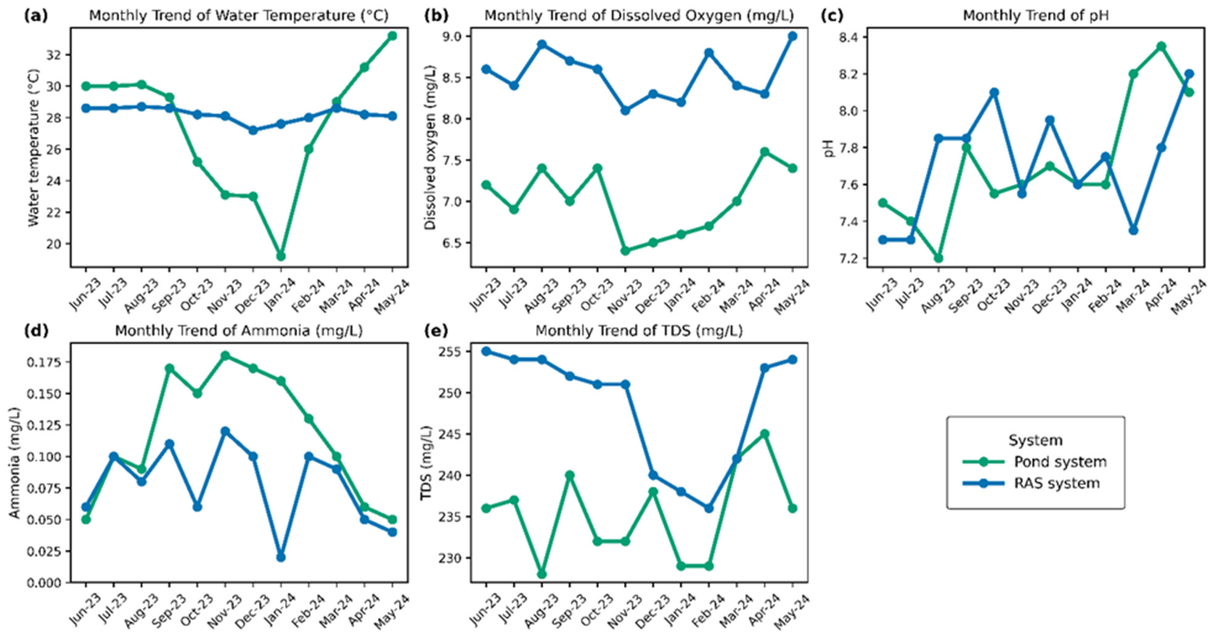
Key water-quality parameters were monitored monthly in the pond and recirculating aquaculture system (RAS) over a one-year period (June 2023 to May 2024), and their trends are summarized in Figure 3a–e. Overall, the RAS maintained a more stable aquatic environment than the pond system, with reduced seasonal variability across most parameters. Water temperature in ponds showed strong seasonal fluctuation (19–34 °C), with the highest values recorded during late spring (April–May). In contrast, RAS temperature remained comparatively stable (27–29 °C) throughout the year, reflecting the controlled nature of the system (Figure 3a). DO was also different between systems: RAS consistently maintained higher and more uniform DO concentrations (8.0–8.9 mg L⁻¹), whereas pond DO varied more widely (6.4–7.6 mg L⁻¹), indicating less stable oxygen availability in open-water conditions (Figure 3b). Ammonia concentrations were generally higher and more variable in ponds (0.04–0.18 mg L⁻¹), suggesting greater accumulation of metabolic waste and lower buffering capacity. RAS ammonia remained lower and more consistent (0.02–0.12 mg L⁻¹), indicating improved waste removal and water treatment efficiency (Figure 3c). Total dissolved solids (TDS) showed relatively similar ranges between systems, but RAS displayed a more regulated pattern over time (Figure 3d). The pH remained within an acceptable range in both systems; however, ponds exhibited a noticeable spring peak (up to 8.37), while RAS maintained a steadier pH across the monitoring period, reflecting tighter control of water chemistry (Figure 3e). Collectively, these trends demonstrate that RAS provided greater stability in temperature, DO, ammonia, and pH compared with pond culture (Figure 3a–e), which is consistent with the higher level of environmental control inherent to recirculating systems.

3.3. Comparative Modeling and Forecasting of Tilapia Broodfish Growth Using ARIMA in Pond and RAS

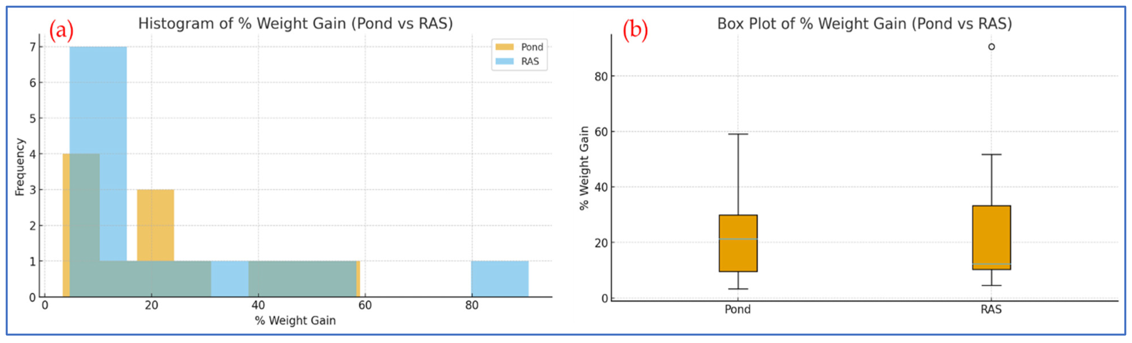
Some basic descriptive statistics of tilapia growth in terms of % weight gain in pond and RAS from June 2023 to May 2024 are presented in

Table 2. Basic descriptive statistics of tilapia % weight gain under pond and RAS (Jun 2023–May 2024).

Indicator	% Weight Gain_Pond	% Weight Gain-RAS
Minimum	3.30	4.62
Maximum	59.03	90.59
1st Quartile (Q1)	9.74	10.78
3rd Quartile (Q3)	33.38	33.63
Mean	23.75	26.69
Median	21.25	13.32
SE Mean	4.88	7.35
Standard Deviation	16.92	25.44
Skewness	0.83	1.58
Kurtosis	0.19	2.11

and Figure 4.

The descriptive analysis of monthly percentage weight gain between pond and RAS revealed distinct differences in growth performance and variability (Table 2 and Figure 4a,b). The mean weight gain in RAS (26.69%) was slightly higher than in ponds (23.75%), indicating a marginally better overall growth performance under the recirculating system. However, the standard deviation in RAS (25.44) was considerably higher than that of ponds (19.92), signifying greater inconsistency in growth across months. This higher variation in RAS was mainly influenced by an extreme outlier in July 2023 (90.59%), as reflected by its strong positive skewness (1.58) and high kurtosis (2.11), which denote a right-skewed and peaked distribution with occasional extreme values. In contrast, pond data showed moderate skewness (0.83) and nearly normal kurtosis (0.19), indicating a more balanced distribution of monthly growth. Quartile comparison revealed that most of the monthly growth values for ponds and RAS fell within 9–33% and 10–33%, respectively, showing overlapping central tendencies but differing spreads. The box plot further confirmed that ponds exhibited a more consistent growth pattern with a relatively higher median and narrower spread, whereas RAS data displayed wider dispersion and evident outliers. Similarly, the histogram illustrated that pond growth was clustered around moderate gains, while RAS showed a longer right tail representing a few months of exceptionally high growth. Overall, while RAS provided higher peak performance, pond systems demonstrated greater stability and uniformity in fish growth across months.

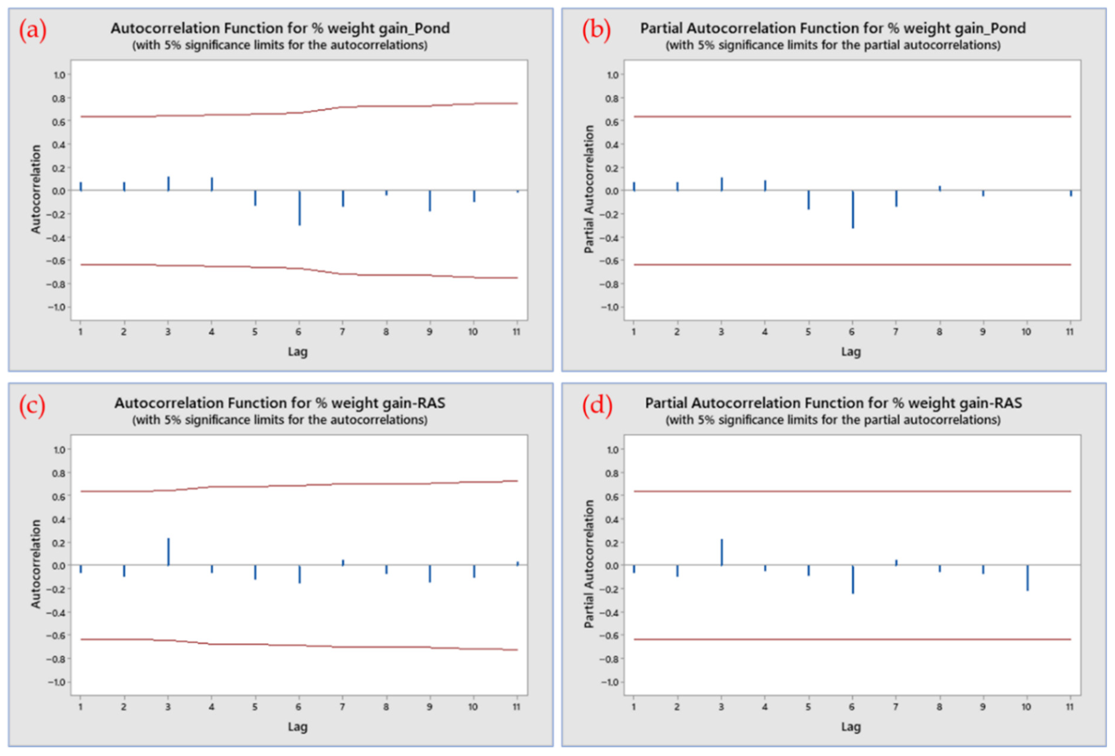
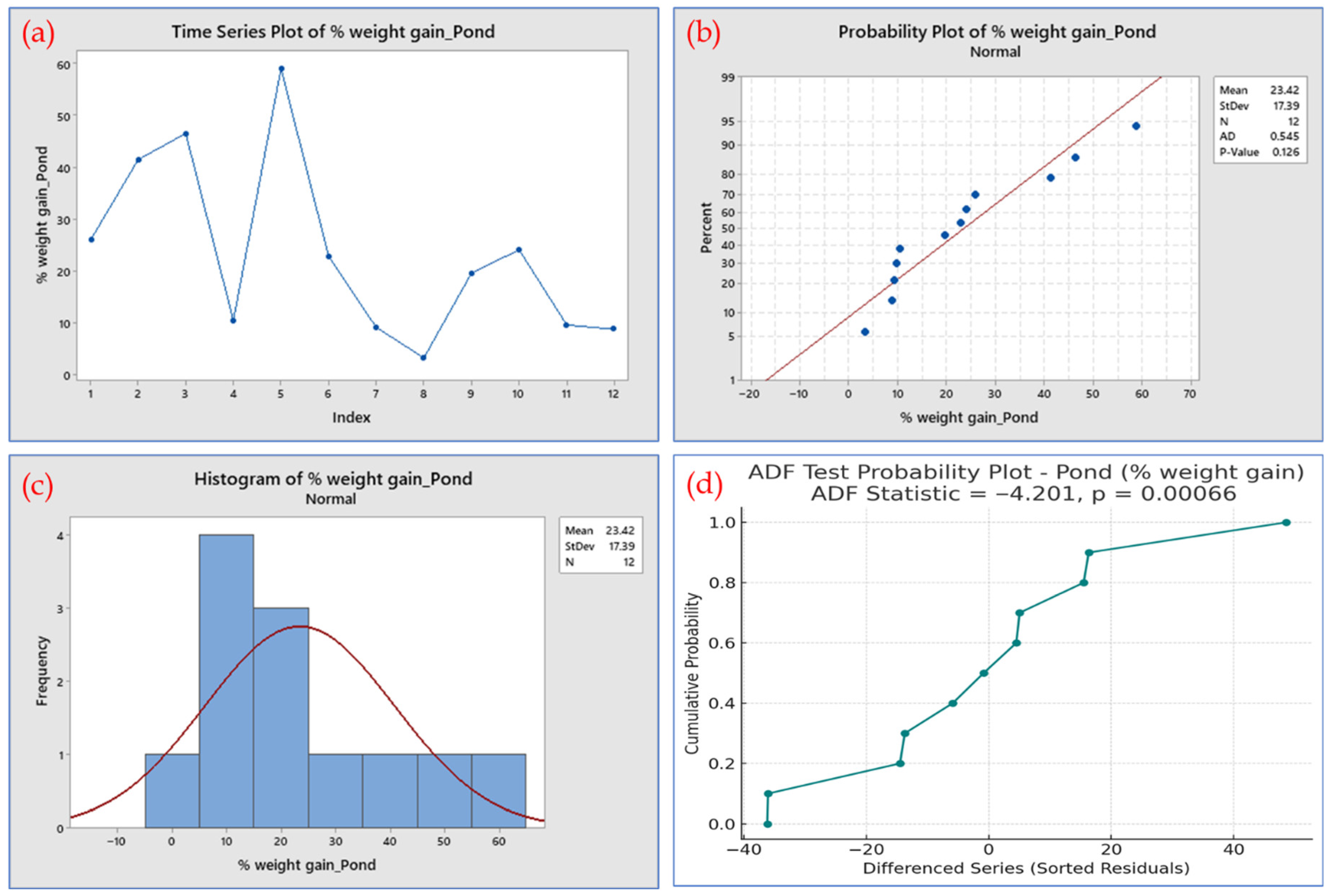
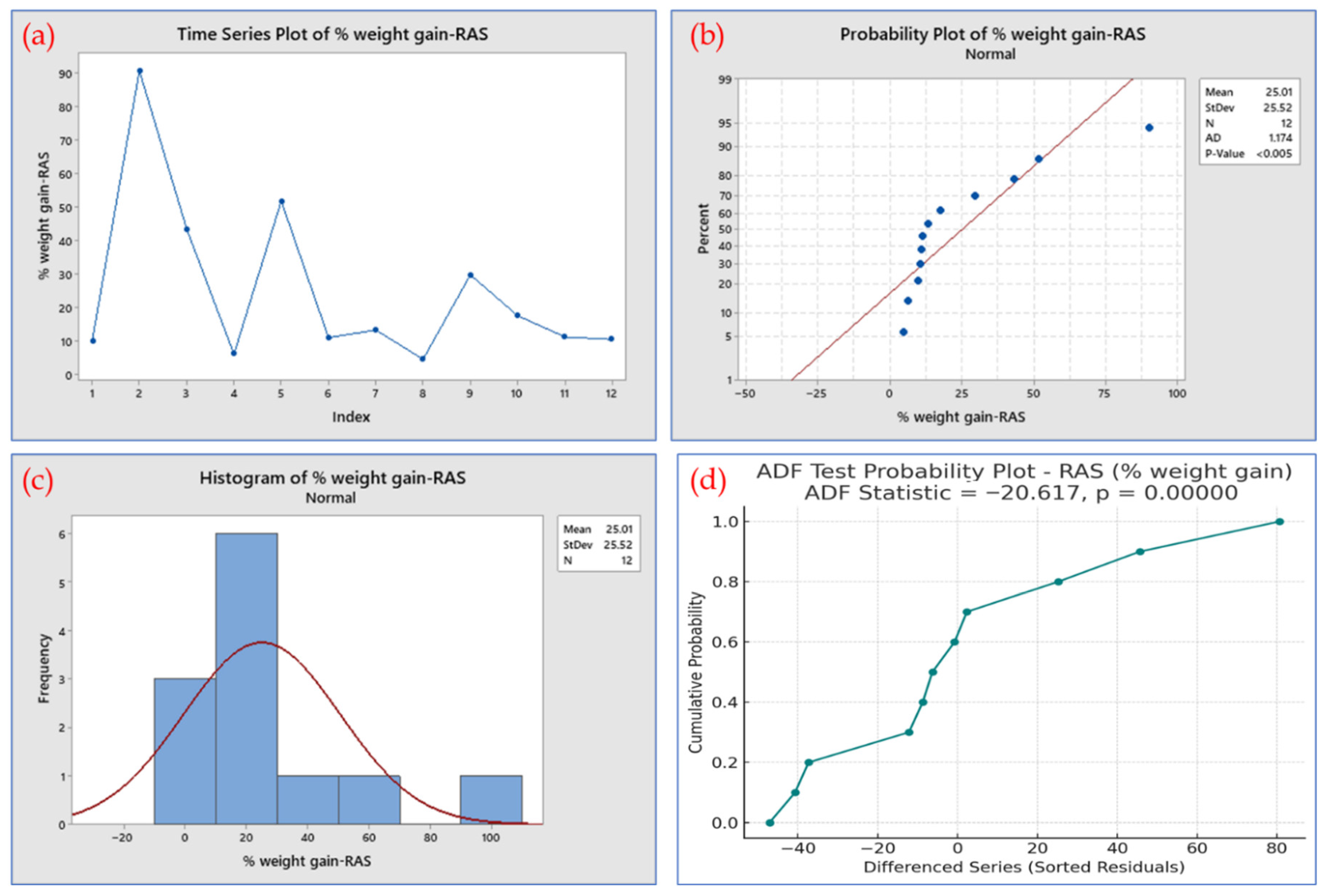
The Anderson–Darling test indicated that pond data did not significantly deviate from normality (p = 0.126), whereas RAS data showed deviation from normality (p < 0.005), likely influenced by an extreme outlier (Figure 5a–d and Figure 6a–d for pond and RAS, respectively). However, the ADF test results for the pond (ADF = −4.2008, p = 0.000657) and RAS (ADF = −20.6174, p = 0.000000) indicated that both datasets were stationary, as the p-values were below the 0.05 significance level. Therefore, no differencing or transformation was required to remove trend components or achieve stationarity prior to ARIMA modeling. Furthermore, the ACF and PACF plots confirmed the stationarity of the data (Figure 7a,b for pond and Figure 7c,d for RAS).

Table 3. Model representation of ARIMA models of % weight gain of tilapia in a pond with BIC values. The best model is indicated with the AIC (*) and BIC (*) values.

Model	RMSE	MAPE	MaxAPE	MAE	MaxAE	BIC	AIC
ARIMA (1,0,1)	17.25	125.79	591.81	14.53	35.34	9.28 *	9.12 *
ARIMA (2,0,2)	16.52	130.96	710.72	14.23	28.47	9.60	9.36
ARIMA (3,0,3)	–	–	–	–	–	–	–
ARIMA (4,0,4)	16.39	105.57	417.60	14.69	32.45	10.38	9.98
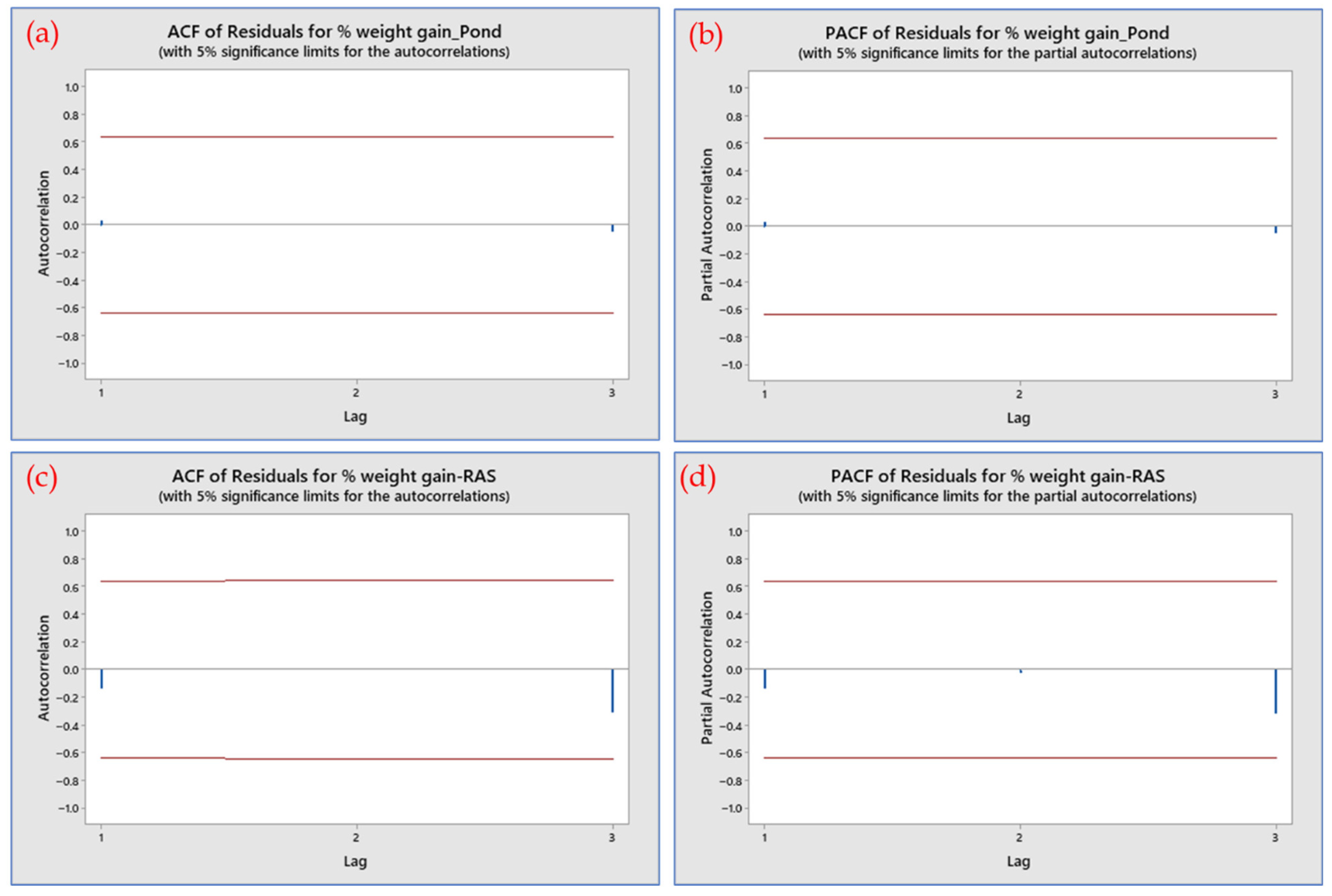
ARIMA (5,0,4)	15.25	64.80	190.20	12.08	34.84	10.15	9.70

and

Table 4. Model representation of ARIMA models of % weight gain of tilapia RAS with BIC values. The best model is indicated with the AIC (*) and BIC (*) values.

Model	RMSE	MAPE	MaxAPE	MAE	MaxAE	BIC	AIC
ARIMA (1,0,1)	24.72	105.36	361.74	18.33	64.21	10.01 *	9.85 *
ARIMA (2,0,2)	24.35	94.72	384.39	17.25	66.04	10.36	10.12
ARIMA (3,0,3)	–	–	–	–	–	–	–
ARIMA (4,0,4)	23.68	106.69	326.63	16.44	64.10	10.97	10.56
ARIMA (5,0,4)	22.94	86.77	208.67	15.71	62.73	11.08	10.64

were used to evaluate the performance of various models based on RMSE, MAPE, MaxAPE, MAE, MaxAE, BIC, and AIC values. Among all the models, ARIMA (1,0,1) was found to have the lowest AIC and BIC values, along with reasonable RMSE, MAPE, MaxAPE, MAE, and MaxAE values, making it the best model for tilapia % weight gain both in the pond and RAS. Although some higher-order models exhibited slightly lower error metrics, ARIMA (1,0,1) was preferred due to its parsimony and lower risk of overfitting, particularly given the small sample size (n = 12). The residual ACF and residual PACF of the model were also analyzed, and it was found that the residuals behaved as white noise. The ACF and PACF values did not exceed the predefined threshold at any lag, indicating an adequate model fit and that the ARIMA model successfully captured the underlying time-series structure (Table 3 for pond and Table 4 for RAS; Figure 8a,b for pond and Figure 8c,d for RAS). Furthermore, the forecasted time series did not exhibit systematic patterns in the residuals, supporting the suitability of ARIMA (1,0,1) as the best-fitting model (Figure 8a–d).

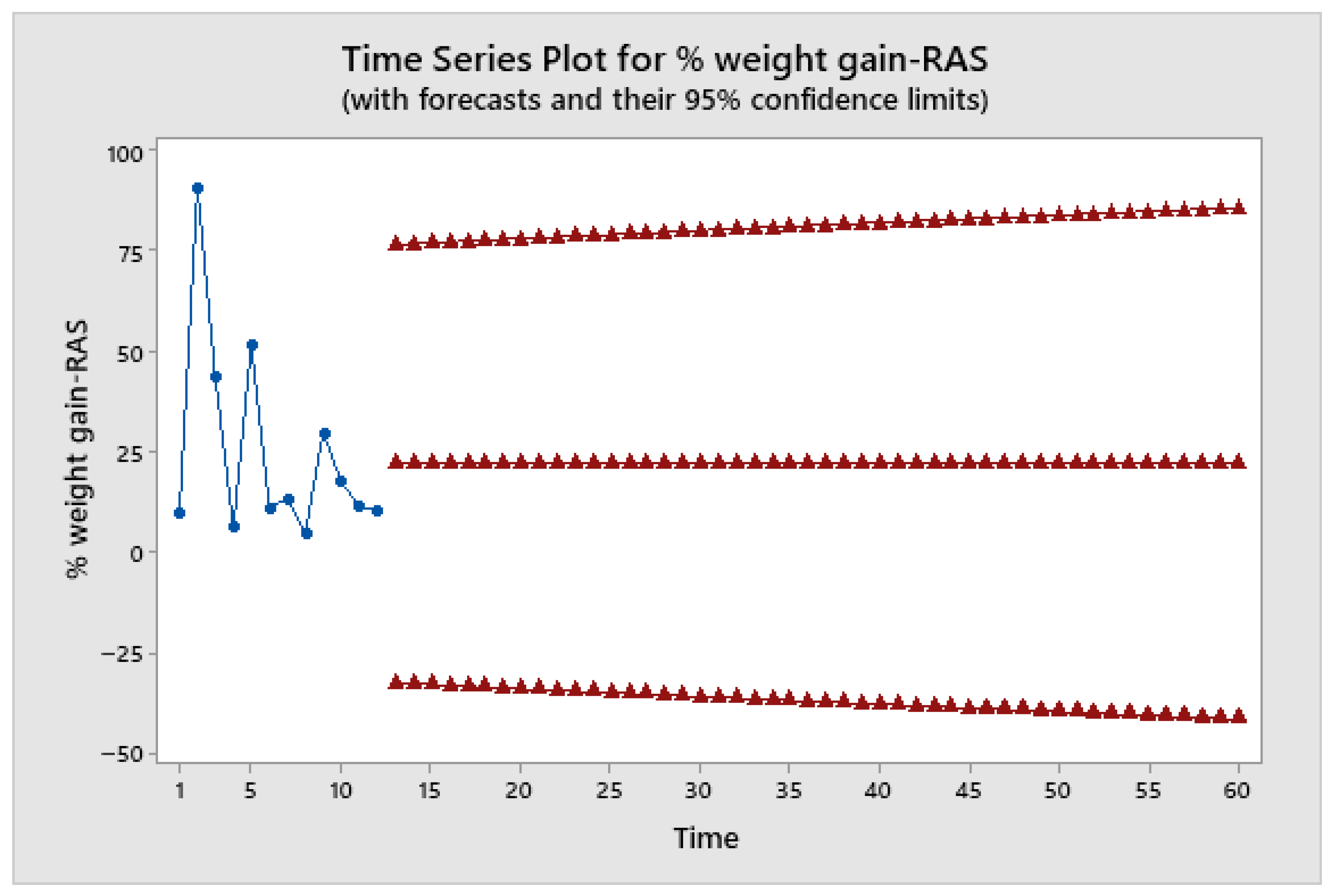
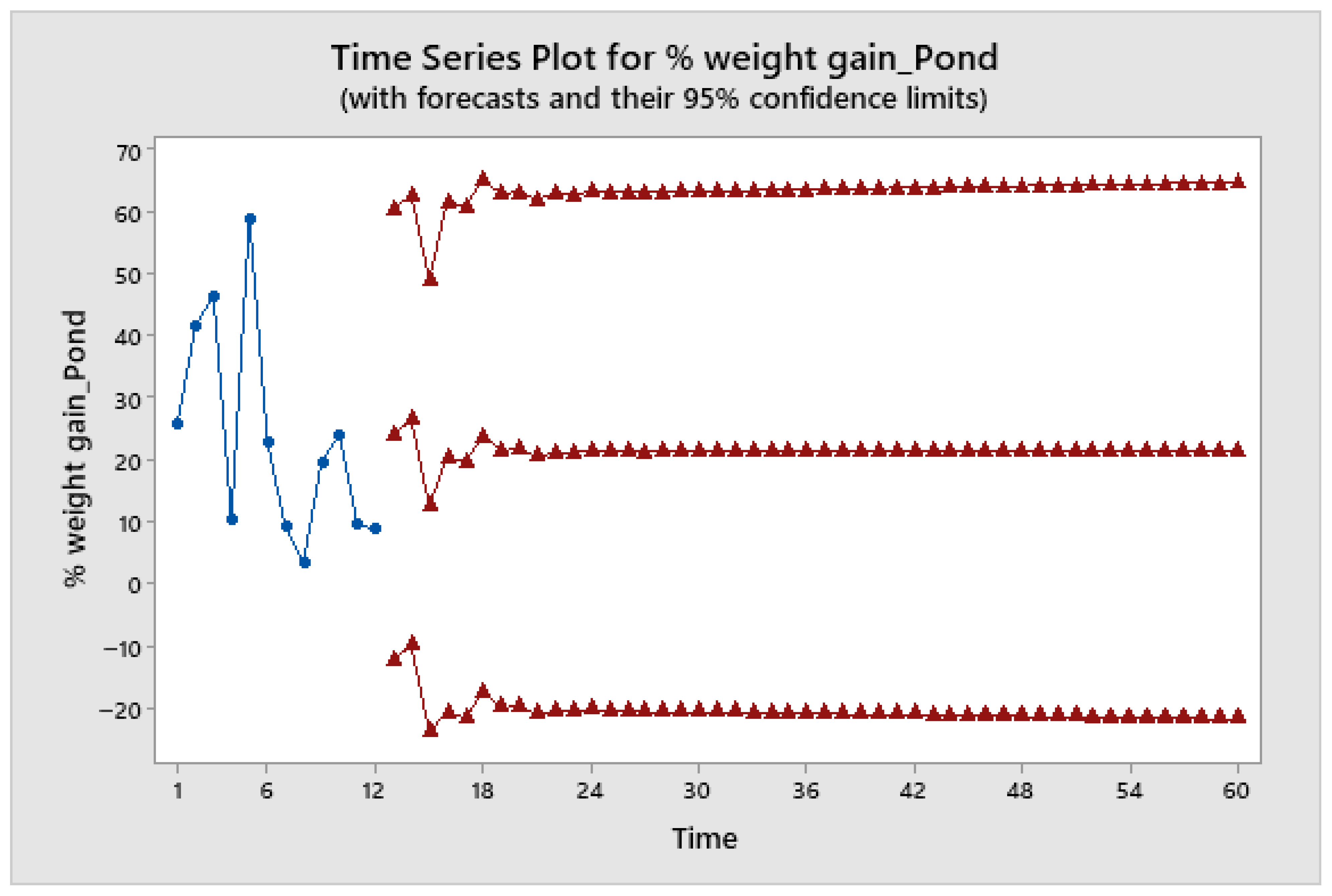
The predicted values for tilapia percentage weight gain in both the pond and RAS over the next four years (

Table A1. Forecast of tilapia % weight gain in the pond up to the end of May 2028.

		95% Limits
Period	Forecast	Lower	Upper
13	23.9832	−12.2429	60.2093
14	26.4718	−9.7799	62.7235
15	12.6944	−23.5829	48.9717
16	20.4436	−20.6543	61.5414
17	19.7108	−21.4375	60.8592
18	23.8115	−17.3873	65.0103
19	21.5156	−19.8147	62.8460
20	21.7401	−19.6311	63.1114
21	20.5284	−20.8837	61.9405
22	21.2174	−20.3361	62.7708
23	21.1574	−20.4394	62.7543
24	21.5243	−20.1160	63.1645
25	21.3263	−20.3385	62.9911
26	21.3509	−20.3564	63.0582
27	21.2487	−20.5012	62.9985
28	21.3143	−20.4846	63.1131
29	21.3137	−20.5278	63.1553
30	21.3509	−20.5334	63.2352
31	21.3382	−20.5869	63.2632
32	21.3451	−20.6225	63.3128
33	21.3409	−20.6693	63.3510
34	21.3514	−20.7018	63.4047
35	21.3562	−20.7396	63.4519
36	21.3642	−20.7741	63.5025
37	21.3679	−20.8127	63.5485
38	21.3733	−20.8498	63.5963
39	21.3777	−20.8878	63.6431
40	21.3834	−20.9246	63.6913
41	21.3886	−20.9617	63.7389
42	21.3941	−20.9986	63.7867
43	21.3992	−21.0358	63.8342
44	21.4044	−21.0729	63.8817
45	21.4096	−21.1100	63.9292
46	21.4149	−21.1470	63.9768
47	21.4201	−21.1840	64.0243
48	21.4254	−21.2210	64.0718
49	21.4306	−21.2580	64.1193
50	21.4359	−21.2949	64.1667
51	21.4411	−21.3318	64.2141
52	21.4464	−21.3687	64.2615
53	21.4517	−21.4056	64.3089
54	21.4569	−21.4424	64.3563
55	21.4622	−21.4793	64.4036
56	21.4674	−21.5161	64.4510
57	21.4727	−21.5529	64.4983
58	21.4780	−21.5896	64.5456
59	21.4832	−21.6264	64.5928
60	21.4885	−21.6631	64.6401

and

Table A2. Forecast of tilapia % weight gain in RAS up to the end of May 2028.

		95% Limits
Period	Forecast	Lower	Upper
13	21.9871	−32.5312	76.5053
14	21.9888	−32.7365	76.7142
15	21.9906	−32.9410	76.9222
16	21.9924	−33.1447	77.1296
17	21.9942	−33.3478	77.3362
18	21.9960	−33.5501	77.5421
19	21.9978	−33.7517	77.7473
20	21.9996	−33.9525	77.9517
21	22.0014	−34.1527	78.1555
22	22.0032	−34.3522	78.3586
23	22.0050	−34.5510	78.5610
24	22.0068	−34.7492	78.7627
25	22.0086	−34.9466	78.9637
26	22.0103	−35.1434	79.1641
27	22.0121	−35.3396	79.3638
28	22.0139	−35.5351	79.5629
29	22.0157	−35.7299	79.7614
30	22.0175	−35.9241	79.9592
31	22.0193	−36.1177	80.1564
32	22.0211	−36.3107	80.3529
33	22.0229	−36.5030	80.5488
34	22.0247	−36.6948	80.7442
35	22.0265	−36.8859	80.9389
36	22.0283	−37.0765	81.1330
37	22.0301	−37.2664	81.3265
38	22.0319	−37.4558	81.5195
39	22.0337	−37.6445	81.7119
40	22.0355	−37.8327	81.9036
41	22.0373	−38.0204	82.0949
42	22.0391	−38.2074	82.2855
43	22.0408	−38.3939	82.4756
44	22.0426	−38.5799	82.6652
45	22.0444	−38.7653	82.8541
46	22.0462	−38.9501	83.0426
47	22.0480	−39.1344	83.2305
48	22.0498	−39.3182	83.4179
49	22.0516	−39.5015	83.6047
50	22.0534	−39.6842	83.7910
51	22.0552	−39.8664	83.9768
52	22.0570	−40.0481	84.1621
53	22.0588	−40.2293	84.3469
54	22.0606	−40.4100	84.5312
55	22.0624	−40.5901	84.7149
56	22.0642	−40.7698	84.8982
57	22.0660	−40.9490	85.0810
58	22.0678	−41.1277	85.2633
59	22.0696	−41.3059	85.4451
60	22.0714	−41.4836	85.6264

; Figure 9 and Figure 10) were found to fall within the 95% confidence limits. The trend in percentage weight gain for the pond system, illustrated in Figure 9 using the ARIMA (1,0,1) model, showed a gradual increase accompanied by apparent fluctuations that may resemble seasonal behavior, although true seasonality cannot be confirmed due to the limited time-series length. In contrast, the trend presented in Figure 10 for the RAS exhibited a gradual increase as well, but with a much less pronounced seasonal pattern. Overall, the RAS demonstrated comparatively better performance, achieving approximately 7% higher weight gain than the pond system, indicating a substantial improvement in percentage weight gain under RAS by the end of May 2028.

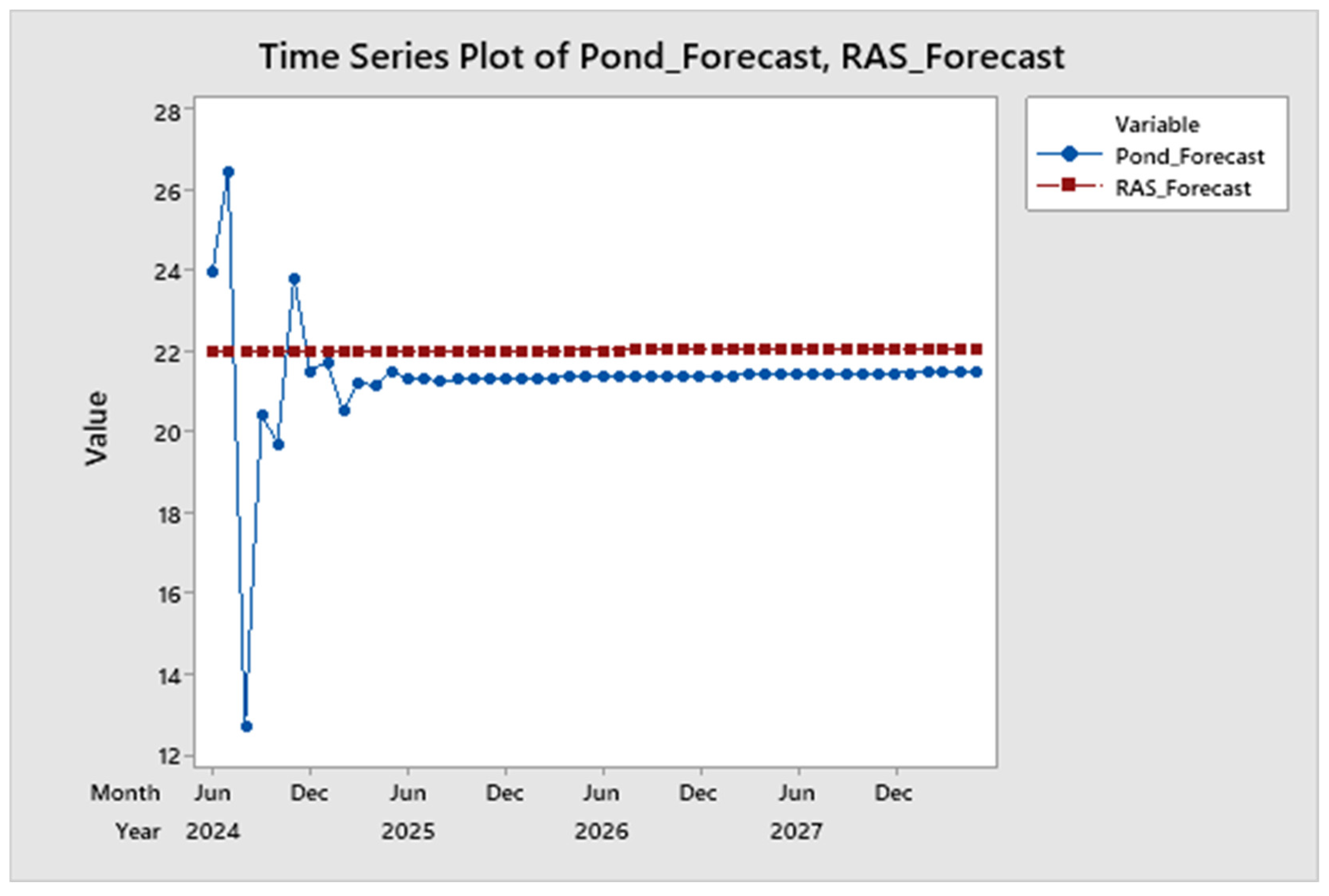
The comparative ARIMA (1,0,1) forecast analysis for tilapia percentage weight gain under pond and RAS conditions revealed clear differences in growth dynamics over the projected period of 48 months (Figure 11). All predicted values remained within the 95% confidence limits, indicating internal consistency of the model rather than independent validation of predictive performance. During the early forecast months, the pond system displayed considerable fluctuations, with predicted % weight gain ranging from 12.69% to 26.47%, reflecting its greater sensitivity to environmental variability. In contrast, the RAS forecast remained highly stable, fluctuating only slightly around 21.99%.

From period month 20 onward, both systems exhibited stabilization, with the pond forecast gradually settling near 21.3%, while the RAS remained consistently higher, averaging approximately 22.0–22.1% throughout the remainder of the forecast horizon. By the end of the projection period (Month 60), the RAS reached a forecasted % weight gain of 22.07%, compared to 21.49% in pond culture, representing a small absolute difference of approximately 0.58 percentage points. This difference corresponds to a modest relative improvement under specific comparative contexts. Overall, the RAS demonstrated a more stable upward trend, narrower variation, and higher sustained growth, reflecting its superior environmental control and efficiency relative to traditional pond-based production.

4. Discussion

The present findings highlight how culture system design (traditional pond vs. RAS) shapes both the biological performance and the statistical behavior of broodfish growth dynamics, which is particularly important when forecasting is intended to support practical management decisions such as feed planning, broodstock conditioning, and production scheduling [23,36,37]. Over the one-year longitudinal observation period, broodfish reared in the RAS demonstrated superior growth performance, better feed conversion efficiency, and higher survival compared with pond-reared fish, highlighting the advantages of controlled culture conditions. These differences align with the widely recognized principle that controlled aquaculture environments can improve feed conversion and growth efficiency when water-quality parameters remain stable and physiological stress is minimized [6,19,20,38,39]. Similar performance advantages under controlled RAS environments have also been reported in recent broodfish nutrition and growth studies, further supporting the importance of stable rearing conditions for improved broodstock performance [40,41]. A mechanistic explanation for these performance differences is supported by the contrasting environmental stability observed between the two systems. The pond environment exhibited pronounced seasonal temperature fluctuations (~19–34 °C), whereas the RAS maintained a relatively stable thermal range (~27–29 °C). Because tilapia growth, appetite, and feed utilization are strongly influenced by temperature, large environmental fluctuations can disrupt metabolic processes and feeding behavior [6,42]. Similarly, dissolved oxygen (DO) concentrations remained consistently higher and more stable in the RAS (~8.0–8.9 mg L⁻¹) compared with ponds (~6.4–7.6 mg L⁻¹), while ammonia levels were lower and less variable in the recirculating system (~0.02–0.12 mg L⁻¹ vs. ~0.04–0.18 mg L⁻¹). Such differences are consistent with established principles of recirculating aquaculture design, where engineered filtration and nitrification processes help control nitrogenous wastes and maintain favorable water-quality conditions [38,43,44,45,46,47,48,49]. Collectively, these environmental characteristics likely contributed to the improved feed conversion efficiency and survival observed in the RAS [10,19,20], and support broader evidence that broodstock and hatchery performance in Bangladesh is strongly influenced by water-quality stability and environmental management [26,50,51,52].

A key contribution is that better average performance did not necessarily mean lower variance in the growth signal used for forecasting. RAS showed a slightly higher mean monthly % weight gain than ponds, but also higher dispersion, influenced by a strong outlier in July 2023. This is important for management interpretation. In ponds, variability often reflects external drivers (weather, plankton dynamics, diurnal oxygen cycles), producing apparent fluctuations that may resemble seasonal behavior, although true seasonality cannot be confirmed due to the limited time-series length, as environmental variability in natural systems may exhibit seasonal tendencies [43,53]. In RAS, variance can be dominated by operational interventions (stocking density changes, biofilter maturation, disinfection cycles, shifts in feeding strategy), which can generate abrupt structural changes even while water parameters appear stable [19,20,47,49]. That distinction matters because forecast errors in RAS may signal management events rather than climate noise, so model monitoring should be paired with an operational log [9,37]. More broadly, this operationally driven variability is consistent with the way technology and management choices shape aquaculture performance trajectories, including through investment and governance patterns in food systems [3,54].

Despite increasing attention to machine learning, this study found that a simple ARIMA-based baseline performed well. Both pond and RAS % weight gain series were stationary by ADF testing (no differencing required), and ARIMA (1,0,1) emerged as the best model according to AIC/BIC and error metrics across systems. In the RAS model comparison table, ARIMA (1,0,1) achieved the minimum AIC/BIC (and competitive RMSE/MAE), reinforcing its selection. This result fits broader forecasting evidence: strong statistical baselines often remain hard to beat in short, noisy time series, particularly when explanatory covariates are incomplete or inconsistently measured [23,24,28,36]. It also aligns with aquaculture forecasting studies from Bangladesh that have successfully applied ARIMA for production, seed supply, and climate-linked management planning [55,56,57].

For decision-making, interpretability is not a minor benefit. An ARIMA model that is easy to diagnose and update can be embedded into routine hatchery workflows, with forecast intervals used as early-warning bounds [23,36]. Unlike descriptive statistics or conventional growth analysis, the ARIMA model captures the temporal dependence between observations and produces forecasts with associated confidence intervals. It should also be noted that no out-of-sample or external validation was performed; therefore, the forecasting performance reflects internal model fit rather than independent predictive accuracy. This provides insight into the expected future growth trajectory and the uncertainty surrounding it, enabling proactive management decisions that cannot be derived from simple historical summaries. It should also be noted that no out-of-sample or external validation was performed; therefore, the forecasting performance reflects internal model fit rather than independent predictive accuracy. When realized growth falls outside the 95% interval, managers can investigate plausible drivers (feed quality, aeration failures, ammonia spikes, disease onset), consistent with health-risk management needs in intensifying systems [58]. In contrast, more complex black-box models may produce marginally lower error but can be harder to troubleshoot and trust under field conditions [23,59]. Recent applied studies using expanded covariates and alternative modeling strategies (including hybrid and facility-specific approaches) also support keeping strong statistical baselines as the reference point before moving to more complex models [26,60]. From a broader perspective, this study also contributes to the aquaculture forecasting literature both conceptually and methodologically. Conceptually, it highlights how contrasting culture systems (pond versus RAS) influence the temporal dynamics and predictability of tilapia broodfish growth. Methodologically, it demonstrates the usefulness of a comparative ARIMA-based framework for evaluating forecasting performance across aquaculture environments and for supporting practical decision-making in broodstock management and production planning.

Under the selected ARIMA (1,0,1), early forecast months showed greater pond fluctuation, whereas RAS remained close to a stable trajectory (around ~22%). By the end of the forecast horizon, the RAS maintained an advantage in predicted % weight gain (about 5–7%). This pattern is consistent with the climate adaptation argument: by stabilizing core drivers (temperature, oxygen, nitrogen), RAS can reduce the amplitude of environmentally forced seasonality [10,61,62]. The long-term forecasts generated in this study are based on several biological and operational assumptions. In particular, the projections assume relatively stable production conditions, including consistent broodstock characteristics, constant stocking density, similar feeding protocols, and stable system performance throughout the forecasting horizon. During the study period, these management practices were maintained consistently to minimize variability in growth dynamics. However, any substantial changes in broodstock composition, stocking density, feeding strategies, or system maintenance could alter growth trajectories and affect forecast reliability. Therefore, the projections should be interpreted as conditional estimates that depend on the continuation of these underlying biological and operational conditions. However, the practical meaning of “better forecasts” depends on the management objective. In ponds, forecasting may primarily support seasonal planning (anticipating low-growth months, scheduling grading/harvest, and preventive aeration), including preparation for plankton-linked instability [43,53]. In RAS, forecasting may be more valuable for detecting operational drift (biofilter performance decline, chronic CO₂ issues, feed-response changes) because climatic seasonality is muted [38,46,47].

Bangladesh’s tilapia sector is increasingly exposed to heat stress, rainfall irregularity, and rapid seasonal transitions that destabilize pond water quality and hatchery performance [42,45,50,63]. These risks are consistent with broader syntheses on climate impacts for fisheries and aquaculture, which emphasize compound stressors and the need for adaptation tools that combine monitoring with forecasting [61,62,64,65]. They also align with global projections that climate change can shift aquaculture production potential and suitability, strengthening the case for controlled systems in some contexts [11]. In this setting, forecasting is not just prediction for prediction’s sake. It is a management layer that can support resource-efficient feeding, improved seed production stability, and earlier responses to stress events, which ultimately helps protect both profitability and food-security contributions of aquaculture [1,2,66].

The present study is based on monthly data over a one-year period (n = 12 observations), which is adequate for baseline modeling but imposes important limitations on statistical inference and forecast reliability. With such a short time series, longer datasets would better capture multi-year climate variability and structural changes [23,61,67], and model diagnostics such as ACF, PACF, and ADF tests may have limited statistical power. The large RAS outlier (July 2023) materially shaped variance and may influence parameter estimates. Robust approaches (outlier-adjusted ARIMA, Bayesian structural time series, or intervention analysis) could be tested [28,36,37]. The study documents detailed climatic and water-quality monitoring, but the main model here is univariate. Given clear mechanistic links between growth, temperature, DO, and ammonia, ARIMAX or dynamic regression could improve interpretability and early warning when covariates are reliably recorded [28,36,42,52]. RAS performance also depends heavily on engineering design, energy reliability, and operator skill, and broader validation across multiple facilities and management regimes is necessary before recommending a single best model as a national decision tool [10,19,20,21].

The evidence supports a balanced conclusion: RAS improved mean growth, feed efficiency, and survival, while pond systems showed comparatively smoother month-to-month biological stability. However, these findings and associated forecasts should be interpreted as exploratory and indicative rather than confirmatory. Both systems were well served by a transparent ARIMA baseline for near-term forecasting [23,24]. The strongest practical pathway forward is a hybrid decision framework: ARIMA/ARIMAX baselines for routine planning and monitoring, complemented by richer covariate logging and targeted machine-learning experiments only after multi-year datasets are available [37,59]. Finally, because long-term sustainability also depends on accurate species identification, breeding control, and broodstock quality assurance, complementary morpho-molecular and genomic approaches remain relevant to hatchery resilience and production reliability [68,69].

Incorporating environmental drivers such as temperature, dissolved oxygen, ammonia, pH, and total dissolved solids could further improve the explanatory power of forecasting models. Including these variables through ARIMAX or dynamic regression frameworks would allow part of the observed growth variability to be attributed to environmental fluctuations rather than relying solely on intrinsic temporal patterns. In pond systems, where environmental conditions vary seasonally, such covariates may increase forecast sensitivity to environmental variability. In contrast, the effect may be smaller in RAS, where water-quality parameters are more tightly regulated, potentially highlighting differences in environmental responsiveness between production systems.

Despite its meaningful findings, this study has several limitations. The analysis was based on a relatively small one-year dataset (n = 12 monthly observations), and therefore, the ARIMA modeling results should be interpreted as exploratory. Long-term projections should therefore be interpreted with caution, as forecast uncertainty increases beyond the observed data range. The projections presented here should be considered conditional estimates assuming relatively stable biological and operational conditions, including consistent broodstock composition. Changes in broodstock structure, such as age, size distribution, or genetic strain, may influence future growth dynamics. In addition, the use of monthly mean values instead of the full sampling dataset may have reduced the ability to capture short-term variability and fine-scale temporal dynamics in growth patterns. In addition, the modeling approach was univariate and did not include potential exogenous drivers, such as environmental and water-quality variables (e.g., temperature, dissolved oxygen, ammonia, and pH), which are known to affect fish growth. The analysis was also conducted at a single facility; therefore, validation across multiple locations, production cycles, and operational conditions would strengthen the robustness and generalizability of future studies. Future research incorporating longer time-series datasets is essential to improve model robustness, enhance diagnostic reliability, and increase confidence in forecasting performance. Incorporating environmental covariates through ARIMAX or dynamic regression models could help evaluate whether the growth advantages observed in RAS persist under varying water-quality conditions. Studies using longer datasets and individual-level observations may also benefit from hierarchical mixed-effects or state-space models to better capture multi-level variability in growth dynamics.

5. Conclusions

This study presents a comparative evaluation of tilapia broodfish growth in traditional pond and recirculating aquaculture systems (RAS) using ARIMA-based time-series modeling and forecasting. The results indicate that the ARIMA (1,0,1) model effectively described growth dynamics and produced reliable forecasts for both culture systems, as supported by stationarity diagnostics, white-noise residuals, and forecast intervals within the 95% confidence limits.

Biologically, tilapia reared in the RAS demonstrated superior performance, including higher overall growth efficiency, improved feed conversion, greater survival, and more stable long-term growth trends compared with pond culture. These outcomes are associated with the greater environmental stability maintained in RAS, particularly with respect to temperature, dissolved oxygen, ammonia, and pH. Although occasional variability was observed in RAS growth patterns, long-term projections indicated more consistent performance relative to pond systems.

Forecast results suggest that RAS is likely to maintain a modest growth advantage over pond culture in future production cycles, highlighting its potential as a more predictable and climate-resilient aquaculture strategy. The findings also indicate that growth variability may arise from different system-specific drivers, including environmental fluctuations in ponds and operational management factors in RAS.

Overall, the study supports the use of transparent statistical forecasting tools such as ARIMA for broodstock management, including feed planning, production monitoring, and early detection of growth deviations. Future research should extend this framework using longer time-series datasets, the incorporation of environmental covariates, and validation across multiple facilities to strengthen forecasting applications in tilapia aquaculture.

References

1. Costello, C.; Cao, L.; Gelcich, S.; Cisneros-Mata, M.Á.; Free, C.M.; Froehlich, H.E.; Golden, C.D.; Ishimura, G.; Maier, J.; Macadam-Somer, I.; et al. The future of food from the sea. Nature 2020, 588, 95–100. [Google Scholar] [CrossRef] [Scilit] [PubMed]
2. Golden, C.D.; Koehn, J.Z.; Shepon, A.; Passarelli, S.; Free, C.M.; Viana, D.F.; Matthey, H.; Eurich, J.G.; Gephart, J.A.; Fluet-Chouinard, E.; et al. Aquatic foods to nourish nations. Nature 2021, 598, 315–320. [Google Scholar] [CrossRef] [Scilit]
3. Crona, B.I.; Wassénius, E.; Jonell, M.; Koehn, J.Z.; Short, R.; Tigchelaar, M.; Daw, T.M.; Golden, C.D.; Gephart, J.A.; Allison, E.H.; et al. Four ways blue foods can help achieve food system ambitions across nations. Nature 2023, 616, 104–112. [Google Scholar] [CrossRef] [Scilit] [PubMed]
4. Datta, P.; Behera, B.; Timsina, J. Achieving sustainable development through agriculture-forestry-livestock nexus in Bangladesh: Synergies and trade-offs. Agric. Syst. 2024, 215, 103854. [Google Scholar] [CrossRef] [Scilit]
5. Chowdhury, M.A.; Shivakoti, G.P.; Salequzzaman, M. A conceptual framework for the sustainability assessment procedures of the shrimp aquaculture industry in coastal Bangladesh. Int. J. Agric. Resour. Gov. Ecol. 2006, 5, 162–184. [Google Scholar] [CrossRef] [Scilit]
6. El-Sayed, A.-F.M. Tilapia Culture, 2nd ed.; Academic Press: New York, NY, USA, 2020. [Google Scholar]
7. Islam, A.H.M.S.; Barman, B.K.; Murshed-e-Jahan, K. Adoption and impact of integrated rice–fish farming system in Bangladesh. Aquaculture 2015, 447, 76–85. [Google Scholar] [CrossRef] [Scilit]
8. Akter, M.; Schrama, J.W.; Rashid, M.M.U.; Verdegem, M. Effect of feed pellet buoyancy and stocking ratio of tilapia on fish and natural food in carp-tilapia polyculture ponds. Aquac. Eng. 2025, 110, 102537. [Google Scholar] [CrossRef] [Scilit]
9. Jahan, R.; Quaiyum, A.; Sarker, B.S.; Belal Hossain, M.; Khalid Bin Jaman, K.M.; Rahman, S. Biodiversity and seasonal abundance of small indigenous fish species (SIS) in the rivers and adjacent beels of Karimganj (Kishoreganj, Bangladesh). Asian J. Anim. Sci. 2014, 8, 38–46. [Google Scholar] [CrossRef] [Scilit]
10. Ahmed, N.; Turchini, G.M. Recirculating aquaculture systems (RAS): Environmental solution and climate change adaptation. J. Clean. Prod. 2021, 297, 126604. [Google Scholar] [CrossRef] [Scilit]
11. Froehlich, H.E.; Gentry, R.R.; Halpern, B.S. Global change in marine aquaculture production potential under climate change. Nat. Ecol. Evol. 2018, 2, 1745–1750. [Google Scholar] [CrossRef] [Scilit]
12. Islam, M.S.; Hoq, M.E. Vulnerability of aquaculture-based fish production systems to the impacts of climate change: Insights from inland waters in Bangladesh. In Bangladesh I: Climate Change Impacts, Mitigation and Adaptation in Developing Countries; Springer International Publishing: Cham, Switzerland, 2019; pp. 67–97. [Google Scholar]
13. Hasan, M.R.; Hossain, M.Y.; Mawa, Z.; Hossain, M.A. Reproductive biology of Heteropneustes fossilis in a wetland ecosystem (Gajner Beel, Bangladesh) in relation to eco-climatic factors: Suggesting a sustainable policy for aquaculture, management and conservation. Saudi J. Biol. Sci. 2022, 29, 1160–1174. [Google Scholar] [CrossRef] [Scilit] [PubMed]
14. Hossain, M.A.; Laboni, T.A.; Khatun, M.S.; Rahman, M.A.; Hossen, M.A.; Rahman, O.; Hossain, M.Y. Exploring the reproductive features of Clupisoma garua from Ganges River, Bangladesh: Insights into eco-climatic factors for sustainable management and advancements in aquaculture practices. Environ. Sci. Pollut. Res. 2024, 31, 34082–34096. [Google Scholar] [CrossRef] [Scilit] [PubMed]
15. Siddique, M.A.B.; Ahmed, I.; Mahalder, B.; Haque, M.M.; Ahammad, A.K.S. Integrated strategies for broodstock management and seed production to mitigate climate and water-quality challenges: A critical and meta-analysis review. Aquac. Fish Fish. 2025, 5, e70158. [Google Scholar] [CrossRef] [Scilit]
16. Siddique, M.A.B.; Mahalder, B.; Haque, M.M.; Ahammad, A.K.S. Impact of climatic and water quality parameters on tilapia (Oreochromis niloticus) broodfish growth: Integrating ARIMA and ARIMAX for precise modeling and forecasting. PLoS ONE 2025, 20, e0313846. [Google Scholar] [CrossRef] [Scilit] [PubMed]
17. Farrier, S.M.; Koupal, K.D.; Burger, P.R.; Wuellner, M.R. Application of a conceptual stocking model for two recreationally important species. Aquac. Fish Fish. 2024, 4, e70006. [Google Scholar] [CrossRef] [Scilit]
18. Saha, J.; Hossain, M.A.; Mamun, M.A.; Islam, M.R.; Alam, M.S. Effects of carbon-nitrogen ratio manipulation on the growth performance, body composition and immunity of stinging catfish Heteropneustes fossilis in a biofloc-based culture system. Aquac. Rep. 2022, 25, 101274. [Google Scholar] [CrossRef] [Scilit]
19. Martins, C.I.M.; Eding, E.H.; Verdegem, M.C.J.; Heinsbroek, L.T.N.; Schneider, O.; Blancheton, J.P.; d’Orbcastel, E.R.; Verreth, J.A.J. New developments in recirculating aquaculture systems in Europe: A perspective on environmental sustainability. Aquac. Eng. 2010, 43, 83–93. [Google Scholar] [CrossRef] [Scilit]
20. Badiola, M.; Mendiola, D.; Bostock, J. Recirculating aquaculture systems (RAS) analysis: Main issues on management and future challenges. Aquac. Eng. 2012, 51, 26–35. [Google Scholar] [CrossRef] [Scilit]
21. Abd El-Hack, M.E.; El-Saadony, M.T.; Nader, M.M.; Salem, H.M.; El-Tahan, A.M.; Soliman, S.M.; Khafaga, A.F. Effect of environmental factors on growth performance of Nile tilapia (Oreochromis niloticus). Int. J. Biometeorol. 2022, 66, 2183–2194. [Google Scholar] [CrossRef] [Scilit]
22. Huq, N. Small scale freshwater ponds in rural Bangladesh: Navigating roles and services. Int. J. Water 2017, 11, 73–85. [Google Scholar] [CrossRef] [Scilit]
23. Makridakis, S.; Spiliotis, E.; Assimakopoulos, V. The M4 competition: Results, findings, conclusion and way forward. Int. J. Forecast. 2020, 36, 54–74. [Google Scholar] [CrossRef] [Scilit]
24. Hyndman, R.J.; Khandakar, Y. Automatic time series forecasting: The forecast package for R. J. Stat. Softw. 2008, 27, 1–22. [Google Scholar] [CrossRef] [Scilit]
25. Parvin, M.F.; Hossain, M.Y.; Sarmin, M.S.; Rahman, O.; Tanjin, S.; Samad, M.A.; Rahman, M.A. Reproductive performance of Asian stinging catfish Heteropneustes fossilis (Bloch 1794) in the Ganges River (NW Bangladesh) in relation to environmental factors. Environ. Sci. Pollut. Res. 2022, 29, 42822–42836. [Google Scholar] [CrossRef] [Scilit] [PubMed]
26. Ivashko, E.; Konovalchikova, E.; Ivashko, V. Aquaculture mathematical modelling review. Aquac. Int. 2025, 33, 281. [Google Scholar] [CrossRef] [Scilit]
27. Faruk, A.R.; Mausumi, M.I.; Anka, I.Z.; Hasan, M.M. Effects of temperature on the egg production and growth of monosex Nile tilapia. Bangladesh Res. Publ. J. 2012, 7, 367–377. [Google Scholar]
28. Box, G.E.P.; Jenkins, G.M. Time Series Analysis: Forecasting and Control; Holden-Day: San Francisco, CA, USA, 1970. [Google Scholar]
29. Schaffer, A.L.; Dobbins, T.A.; Pearson, S.A. Interrupted time series analysis using autoregressive integrated moving average (ARIMA) models: A guide for evaluating large-scale health interventions. BMC Med. Res. Methodol. 2021, 21, 58. [Google Scholar] [CrossRef] [Scilit] [PubMed]
30. Siddique, M.A.B.; Ahmed, I.; Mahalder, B.; Haque, M.M.; Akhtar, S.; Ahammad, A.K.S. Forecasting fish seed production in Bangladesh’s private hatcheries using ARIMA. Aquac. Res. 2025, 2025, 7871274. [Google Scholar] [CrossRef] [Scilit]
31. Ospina, R.; Gondim, J.A.M.; Leiva, V.; Castro, C. An overview of forecast analysis with ARIMA models during the COVID-19 pandemic: Methodology and case study in Brazil. Mathematics 2023, 11, 3069. [Google Scholar] [CrossRef] [Scilit]
32. Chitra, N.; Shanmathi, R.; Rajesh, R. Application of ARIMA model using SPSS software—A case study in supply chain management. Int. J. Sci. Technol. Manag. 2015, 1, 206–215. [Google Scholar]
33. Nazmi, H.; Siau, N.Z.; Bramantoro, A.; Suhaili, W.S. Predictive modeling of marine fish production in Brunei Darussalam’s aquaculture sector: A comparative analysis of machine learning and statistical techniques. Int. J. Adv. Appl. Sci. 2023, 10, 109–126. [Google Scholar] [CrossRef] [Scilit]
34. Mishra, P.; Al Khatib, A.M.G.; Sardar, I.; Mohammed, J.; Karakaya, K.; Dash, A.; Ray, M.; Narsimhaiah, L.; Dubey, A. Modeling and forecasting of sugarcane production in India. Sugar Tech. 2021, 23, 1317–1324. [Google Scholar] [CrossRef] [Scilit]
35. Boruah, B.B.; Roy, P.; Dutta, A.; Hazarika, B.B. Forecasting marine and total fish production in India using ARIMA model. Indian J. Econ. Bus. 2020, 19, 161–174. [Google Scholar]
36. Hyndman, R.J.; Athanasopoulos, G. Forecasting: Principles and Practice, 2nd ed.; OTexts: Melbourne, Australia, 2018. [Google Scholar]
37. Taylor, S.J.; Letham, B. Forecasting at scale. Am. Stat. 2018, 72, 37–45. [Google Scholar] [CrossRef] [Scilit]
38. Timmons, M.B.; Ebeling, J.M. Recirculating Aquaculture, 3rd ed.; Cayuga Aqua Ventures: Ithaca, NY, USA, 2010. [Google Scholar]
39. D’oRbcastel, E.R.; Ruyet, J.P.-L.; Le Bayon, N.; Blancheton, J.-P. Comparative growth and welfare in rainbow trout reared in recirculating and flow-through rearing systems. Aquac. Eng. 2009, 40, 79–86. [Google Scholar] [CrossRef] [Scilit]
40. Keyvanshokooh, S.; Salati, A.P.; Ghasemi, A.; Nazemroaya, S.; Houshmand, H.; Mozanzadeh, M.T. Reproductive benefits of dietary selenium nanoparticles (SeNPs) in Asian seabass (Lates calcarifer) male broodstock. Mar. Biotechnol. 2025, 27, 45. [Google Scholar] [CrossRef] [Scilit]
41. Mohtashemipour, H.; Mohammadian, T.; Torfi Mozanzadeh, M.; Mesbah, M.; Jangaran Nejad, A. Dietary selenium nanoparticles improved growth and health indices in Asian seabass (Lates calcarifer) juveniles reared in high saline water. Aquac. Nutr. 2024, 2024, 7480824. [Google Scholar] [CrossRef] [Scilit]
42. Siddique, M.A.B.; Mahalder, B.; Haque, M.M.; Ahammed, A.K.S. Impact of climatic factors on water quality parameters in tilapia broodfish ponds and predictive modeling of pond water temperature with ARIMAX. Heliyon 2024, 10, e37717. [Google Scholar] [CrossRef] [Scilit]
43. Boyd, C.E.; Tucker, C.S. Pond Aquaculture Water Quality Management; Springer: New York, NY, USA, 1998. [Google Scholar] [CrossRef] [Scilit]
44. Froehlich, H.E.; Gentry, R.R.; Halpern, B.S. Synthesis and comparative analysis of physiological tolerance and life-history growth traits of marine aquaculture species. Aquaculture 2016, 460, 75–82. [Google Scholar] [CrossRef] [Scilit]
45. Ahmed, N.; Diana, J.S. Does climate change matter for freshwater aquaculture in Bangladesh? Reg. Environ. Change 2016, 16, 1659–1669. [Google Scholar] [CrossRef] [Scilit]
46. Summerfelt, S.T.; Vinci, B.J.; Piedrahita, R.H. Oxygenation and carbon dioxide control in water reuse systems. Aquac. Eng. 2000, 22, 87–108. [Google Scholar] [CrossRef] [Scilit]
47. Summerfelt, S.T. Design and management of conventional fluidized-sand biofilters. Aquac. Eng. 2006, 34, 275–302. [Google Scholar] [CrossRef] [Scilit]
48. Wortman, B.; Wheaton, F. Temperature effects on biodrum nitrification. Aquac. Eng. 1991, 10, 183–205. [Google Scholar] [CrossRef] [Scilit]
49. Hagopian, D.S.; Riley, J.G. A closer look at the bacteriology of nitrification. Aquac. Eng. 1998, 18, 223–244. [Google Scholar] [CrossRef] [Scilit]
50. Alam, E.; Mallick, B. Climate change perceptions, impacts and adaptation practices of fishers in southeast Bangladesh coast. Int. J. Clim. Change Strateg. Manag. 2022, 14, 191–211. [Google Scholar] [CrossRef] [Scilit]
51. Bezerra, V.M.; Reis, G.P.A.; de Melo, C.L.; Menezes, W.F.; dos Santos, B.D.; Ferreira, M.P.; de Alvarenga, É.R. A long-term high temperature on young Nile tilapia females affects its urogenital papilla morphology and future reproductive performance. Aquaculture 2025, 595, 741666. [Google Scholar] [CrossRef] [Scilit]
52. Siddique, M.A.B.; Talukdar, M.M.N.; Ahmed, I.; Shimul, M.S.T.; Younos, I.B.; Mahalder, B.; Ahammad, A.S. Effects of climatic and water quality changes on growth and reproduction of Pangasianodon hypophthalmus in traditional pond culture systems. Egypt. J. Aquat. Res. 2026, 52, 16–26. [Google Scholar] [CrossRef] [Scilit]
53. Karmakar, S.R.; Hossain, M.B.; Sarker, M.M.; Nur, A.A.U.; Habib, A.; Paray, B.A.; Al-Sadoon, M.K.; Gulnaz, A.; Arai, T. Diversity and community structure of zooplankton in homestead ponds of a tropical coastal area. Diversity 2022, 14, 755. [Google Scholar] [CrossRef] [Scilit]
54. Hicks, C.C.; Cohen, P.J.; Graham, N.A.J.; Nash, K.L.; Allison, E.H.; D’Lima, C.; Mills, D.J.; Roscher, M.; Thilsted, S.H.; Thorne-Lyman, A.L.; et al. Harnessing global fisheries to tackle micronutrient deficiencies. Nature 2019, 574, 95–98. [Google Scholar] [CrossRef] [Scilit] [PubMed]
55. Raman, R.K.; Sathianandan, T.V.; Sharma, A.P.; Mohanty, B.P. Modelling and forecasting marine fish production in Odisha using seasonal ARIMA model. Natl. Acad. Sci. Lett. 2017, 40, 393–397. [Google Scholar] [CrossRef] [Scilit]
56. Siddique, M.A.B.; Mahalder, B.; Haque, M.M.; Shohan, M.H.; Biswas, J.C.; Akhtar, S.; Ahammad, A.K.S. Forecasting of tilapia production in Bangladesh using ARIMA model. Heliyon 2024, 10, e27111. [Google Scholar] [CrossRef] [Scilit] [PubMed]
57. Siddique, M.A.B.; Mahalder, B.; Haque, M.M.; Ahamad, A.K.S. Forecasting air temperature and rainfall in Mymensingh, Bangladesh with ARIMA: Implications for aquaculture management. Egypt. J. Aquat. Res. 2025, 51, 294–303. [Google Scholar] [CrossRef] [Scilit]
58. Kumar, V.; Roy, S.; Behera, B.K.; Bossier, P.; Das, B.K. Acute hepatopancreatic necrosis disease (AHPND): Virulence, pathogenesis and mitigation strategies in shrimp aquaculture. Toxins 2021, 13, 524. [Google Scholar] [CrossRef] [Scilit] [PubMed]
59. Siddique, M.A.B.; Ahmed, I.; Mahalder, B.; Akhtar, S.; Haque, M.M.; Ahammad, A.K.S. Innovative approaches to modelling and forecasting in fisheries: A critical review. Aquac. Fish Fish. 2026, 6, e70173. [Google Scholar] [CrossRef] [Scilit]
60. Alday, P.M. How much baseline correction do we need in ERP research? Extended GLM model can replace baseline correction while lifting its limits. Psychophysiology 2019, 56, e13451. [Google Scholar] [CrossRef] [Scilit]
61. Intergovernmental Panel on Climate Change (IPCC). Climate Change 2022—Impacts, Adaptation and Vulnerability: Working Group II Contribution to the Sixth Assessment Report of the Intergovernmental Panel on Climate Change; Cambridge University Press: Cambridge, UK, 2022. [Google Scholar]
62. Barange, M.; Bahri, T.; Beveridge, M.C.M.; Cochrane, K.L.; Funge-Smith, S.; Poulain, F. Impacts of Climate Change on Fisheries and Aquaculture: Synthesis of Current Knowledge, Adaptation and Mitigation Options; FAO Fisheries and Aquaculture Technical Paper No. 627; FAO: Rome, Italy, 2018. [Google Scholar]
63. Sihombing, C.U.A.; Fauzi, M.; Windarti, W. Survival and growth of Pangasianodon hypophthalmus cultured under controlled photoperiod. Depik 2021, 10, 98–102. [Google Scholar] [CrossRef] [Scilit]
64. Ray, S.K.; Dutta, S.; Pailan, G.H.; Suresh, V.R.; Dasgupta, S. Hormonal signatures of gonad maturity and seasonality of spawning in migrating hilsa, Tenualosa ilisha. Environ. Biol. Fishes 2022, 105, 37–53. [Google Scholar] [CrossRef] [Scilit]
65. Naylor, R.L.; Kishore, A.; Sumaila, U.R.; Issifu, I.; Hunter, B.P.; Belton, B.; Bush, S.R.; Cao, L.; Gelcich, S.; Gephart, J.A.; et al. Blue food demand across geographic and temporal scales. Nat. Commun. 2021, 12, 5413. [Google Scholar] [CrossRef] [Scilit]
66. FAO. The State of World Fisheries and Aquaculture 2024: Blue Transformation in Action; FAO: Rome, Italy, 2024. [Google Scholar]
67. Bhaumik, U. Review of global studies on food, growth and maturity profile of Indian shad (Tenualosa ilisha). Int. J. Curr. Res. Acad. Rev. 2015, 3, 127–139. [Google Scholar]
68. Shafi, M.E. A comprehensive review of summer mortality syndrome in fish: Causes, climate impact, and mitigation strategies. J. Adv. Vet. Anim. Res. 2025, 12, 890. [Google Scholar] [CrossRef] [Scilit]
69. Wang, Y.T.; Lee, C.Y.; Chan, C.H.; Lai, L.C.; Tsai, M.H.; Chuang, E.Y.; Chen, L.H. Characterizing immune responses of grey mullet (Mugil cephalus) to Nocardia seriolae ex vivo and in vivo. Aquac. Int. 2025, 33, 112. [Google Scholar] [CrossRef] [Scilit]
Figure 1. A schematic diagram of ARIMA modeling and forecasting, which is adapted from the Box–Jenkins [28] methodology and Siddique et al. [30].
Aquacj 06 00013 g001
Figure 2. Comparative growth performance of tilapia in pond and RAS; (a) length, (b) weight, (c) % length gain, (d) % weight gain, (e) FCR, and (f) SGR.
Aquacj 06 00013 g002
Figure 3. Monthly trends in water-quality parameters in the pond and recirculating aquaculture system (RAS) from June 2023 to May 2024: (a) water temperature (°C), (b) dissolved oxygen (mg L−1), (c) ammonia (mg L−1), (d) total dissolved solids (mg L−1), and (e) pH.
Aquacj 06 00013 g003
Figure 4. Histogram and box plot of basic descriptive data statistics of % weight gain in pond (a) and RAS (b).
Aquacj 06 00013 g004
Figure 5. Normality and stationarity diagnostics of % weight gain for pond: (a) time-series plot (blue line with markers shows observed values); (b) normal probability plot (blue dots represent data, red line indicates normal fit); (c) histogram (blue bars show frequency, red curve indicates fitted normal distribution); and (d) ADF test plot (line represents cumulative probability of the differenced series).
Aquacj 06 00013 g005
Figure 6. Normality and stationarity diagnostics of % weight gain for RAS: (a) time-series plot (blue line with markers shows observed values); (b) normal probability plot (blue dots represent data, red line indicates normal fit); (c) histogram (blue bars show frequency, red curve indicates fitted normal distribution); and (d) ADF test plot (line represents cumulative probability of the differenced series).
Aquacj 06 00013 g006
Figure 7. Autocorrelation and partial autocorrelation analysis of % weight gain for tilapia: (a) autocorrelation function (ACF) for pond data; (b) partial autocorrelation function (PACF) for pond data; (c) autocorrelation function (ACF) for RAS data; and (d) partial autocorrelation function (PACF) for RAS data. Blue bars represent correlation coefficients at different lags, and red lines indicate the 5% significance limits.
Aquacj 06 00013 g007
Figure 8. Residual ACF and PACF plots for percentage weight gain of tilapia in pond (a,b) and RAS (c,d). Blue spikes indicate the autocorrelation/partial autocorrelation coefficients at each lag, red horizontal lines show the 5% significance limits, and the gray horizontal line denotes zero correlation.
Aquacj 06 00013 g008
Figure 9. Forecasting of tilapia % weight gain in the pond system up to the end of May 2028. The central line represents the forecasted values, while the upper and lower lines indicate the upper confidence limit (UCL) and lower confidence limit (LCL) corresponding to the 95% confidence interval.
Aquacj 06 00013 g009
Figure 10. Forecasting of tilapia % weight gain in RAS up to the end of May 2028. The central line represents the forecasted values, while the upper and lower lines indicate the upper confidence limit (UCL) and lower confidence limit (LCL) corresponding to the 95% confidence interval.
Aquacj 06 00013 g010
Figure 11. A comparative forecast of % weight gain between the pond and RAS using ARIMA (1,0,1).
Aquacj 06 00013 g011