Chebfun in Numerical Analytic Continuation of Solutions to Second Order BVPs on Unbounded Domains

Abstract

The well-known shooting algorithm has produced important results in solving various linear as well as nonlinear BVPs, defined on unbounded intervals, but has become obsolete. The main difficulty lies in the numerical handling of the domain’s infiniteness. This paper presents a three-step strategy that significantly improves the traditional truncation algorithm. It consists of Chebyshev collocation, implemented as Chebfun, in conjunction with rational AAA interpolation and analytic continuation. Furthermore, and more importantly, this approach enables us to provide a thorough analysis of both possible errors in dealing with and the hidden singularities of some BVPs of real interest. A singular second-order eigenvalue problem and a fourth-order nonlinear degenerate parabolic equation, all defined on the real axis, are considered. For the latter, Chebfun provides properties-preserving solutions. Travelling wave solutions are also studied. They are highly nonlinear BVPs. The problem arises from the analysis of thin viscous film flows down an inclined plane under the competing stress due to the surface tension gradients and gravity, a long-standing concern of ours. By extending the solutions to these problems in the complex plane, we observe that the complex poles do not influence their behaviour. On the other hand, the real ones involve singularities and indicate how long solutions can be extended through continuity.

1. Introduction

No nonlinear differential equation relevant to engineering, it seems, is too simple to be uncomplicated off the real axis.

[1]

This quote incites the study of the location of complex singularities of BVPs attached to nonlinear differential equations. This study underlies this work.

Moreover, some authors have argued that a complete understanding of the dynamics of almost all nonlinear systems is only possible through an analysis of complex singularities [2,3,4]. In this paper, we will focus on cases where a solution has been computed numerically, and it is desired to explore how the solution changes if a variable becomes complex. Some of the considered solutions resolve nonlinear systems that come from the particularisation of the Navier-Stokes system, are defined on unbounded domains and describe various viscous flows in thin layers.

A three-step strategy is proposed for the computation of singularities in nonlinear BVPs defined on unbounded intervals. The first step involves numerically solving the BVP using the Chebyshev collocation spectral method. The second step involves a rational extrapolation technique for the solution, utilising the best or near-best rational interpolation algorithm AAA (Adaptive Antoulas-Anderson) [5]. The third step involves numerical analytical continuation into the complex plane. In other words, it is desired to explore how the solution changes if a variable becomes complex. Typically, the BVPs’ solutions are real analytic, and it may be of interest to understand what happens on the complex plane. A particular goal, not completely achieved quite yet, is to classify the singularities, i.e., whether they are poles, and if so, of what order? Are they branch points, or even essential singularities?

To achieve this, we will use two classes of examples that are very different from each other.

In the first class, as a typical example, we consider the singular Sturm-Liouville (SL for short) problem:

$$\begin{array}{c}-u_{xx}\left(x\right)+c_1\left(x\right)u\left(x\right)=\lambda c_2\left(x\right)u\left(x\right),-\infty <x<\infty .\\ u\left(\pm \infty \right)=0.\end{array}$$

(1)

where $c_1\left(x\right):=x^2+{\displaystyle \frac{\tanh \left(x\right)}{log\left(x^2+11/10\right)}}$ and $c_2\left(x\right):={\displaystyle \frac{1}{x^2+\cos \left(x\right)}}$.

The singularity of this problem comes from the singularities of the coefficients $c_1\left(x\right)$ and $c_2\left(x\right)$, as well as from the fact that its domain of definition is infinite.

The problem is solved, but not completely, by two sinc type collocation methods in the paper [6].

The second topic of interest is the flow of thin liquid films (layers) driven by the competing effects of a surface tension gradient and gravity, which reads:

$$h_t+{\left(f\left(h\right)\right)}_x+{\left(h^3{h}_{xxx}\right)}_x+D{\left(h^3{h}_x\right)}_x=0,-\infty <x<\infty ,$$

(2)

where $h(x,t)$ is the film profile (film above the inclined plane, as a function of distance x down the plane, and time t) and $D={\left({\displaystyle \frac{9}{4}}{\displaystyle \frac{{\tau }^2}{\gamma \rho g}}\right)}^{1/3}{\displaystyle \frac{cot\alpha }{{\left(sin\alpha \right)}^{1/3}}}$. In this non-dimensional parameter, $\alpha$ represents the slope of the plane, $\tau$ denotes the surface tension gradient, $\rho$ the density of the liquid, g the magnitude of the gravitational acceleration vector and $\gamma$ the surface tension of the liquid. The function $f\left(h\right)$ is the so-called flux function, convex or not, that is, generally a polynomial of $h$.

Although dependence on an additional transverse spatial variable y is important, in this paper we take h to be independent of y.

In this form, this equation has been studied theoretically (existence and uniqueness) and numerically (using finite differences) in [7,8,9] in the context of coating flows.

Our study is totally complementary to these works. Thus, we briefly compare our procedure for studying the complex singularities of BVPs with some approaches found in the literature.

There exists a quite large body of work devoted to the computation of singular solutions of nonlinear PDEs. We will only cite two works that we find significant, namely [2,10]. In the former quoted paper, the author introduces a strategy which starts with a Fourier spectral method to solve the PDE and then, as a second step, a numerical analytical continuation into the complex plane based on the epsilon algorithm to sum the Fourier series is used. To obtain information on the nature and location of the singularity, the author examines the rate of decay of the Fourier coefficients. This procedure computes the solution directly in the complex domain. In the latter paper, the authors provide a review of the computational methods used to characterise the complex singularities developed by some relevant PDEs. Last but not least, in [11], the authors analyse the Burger’s equation in the complex plane.

In the present paper, we explore the central problem in the area, i.e., analytic continuation, using two examples of very different complexities, in the spirit exposed in the papers [4,12,13].

As is mentioned in [4] “the analytic continuation problem is ill-posed a priori, since the result depends discontinuously on the data, but becomes well-posed, though with infinite condition numbers, if we confine attention to a simply connected subset of a domain such as a disc or a strip where it is known that a function is bounded”.

We will use a rational approximation that is, computed numerically using the AAA algorithm, and we will show how we can view an analytic continuation of a solution in the complex plane from numerical data on the real line. Generally speaking, the AAA algorithm can be unstable, but it has the advantage of working remarkably well as a black box near-best rational approximator on complex sets (intervals, discs, irregular domains).

Thus, in short, the AAA algorithm takes some nodes $z_j$ in a specified domain and the corresponding function values $f_j$. It returns a rational function $r\left(z\right)$ that can be used to approximate the original function for values z in the complex plane. Actually, we can use this algorithm to provide an approximate analytic continuation of solutions to (1) and (2) from a numerical solution on the real line.

However, we must note that (the numerical) analytic continuation is generally ill-posed and becomes much less accurate the further we are from the real line. Although rational approximations will usually not give accurate information, especially since singularities of solutions to BVPs in the complex plane are usually more complicated than just poles, they are often good at giving a rough idea of the nature of such singularities near the domain of approximation.

We organise the paper in the following way: In Section 2, we solve a singular SL problem, i.e., we find the first three eigenpairs and establish the convergence rate for the first three eigenvectors. Then, we show that the complex poles do not influence computing with Chebfun. The dependence of the eigenvalues on the length X of integration is studied through the relative drift. Chebfun correctly computes a large number of eigenpairs, whereas DESCM and conventional sinc collocation compute only the first pair. In Section 3, we consider a fourth-order nonlinear degenerate parabolic equation that models a thin viscous film on an inclined plane due to the competing action of gravity and Marangoni stress. First, we show that the Chebfun solutions preserve some nonnegativity properties of solutions. Then we consider travelling wave-type solutions, which means solving a third-order nonlinear and singular BVP. When analysed in the complex plane, we notice that this equation has both complex and real poles. Only the latter leads to branch-point singularities. In the last subsection of this section, we analyse the complex singularities when the gravity is neglected, i.e., the fluid flow is only due to the Marangoni stress. In Section 4, we discuss the validity of our strategy for studying the singularities of PDEs and ODEs. In Section 5, we recognise that, even though the followed strategy is beset with risks, such as spurious poles, some defects, ill-conditioning, and possible numerical instabilities, we are sufficiently satisfied with the results obtained here to continue the investigation.

2. A Singular SL Problem on the Real Axis

2.1. Complex Singularities of the SL Problem

Equation (1) has several points at which the coefficient functions are not analytic. Both coefficient functions $c_1\left(x\right)$ and $c_2\left(x\right)$ from (1) have purely imaginary poles.

The solutions (eigenfunctions) $v_i\left(x\right),i=1,2,3,\dots$ have the following asymptotic behaviour near the boundary points:

$$v_i\left(x\right)\sim A{\left|x\right|}^{-1/2}log\left(-{\displaystyle \frac{1}{2}}{x}^2\right),\left|x\right|\to \infty ,$$

(3)

for some positive constant A (see [6]).

2.2. Chebfun Solution to SL Problem

Throughout the work, we make use of the Chebyshev technology implemented through the open source programming environment Chebfun. It is based on the MATLAB R2023b platform and is designed for computation using functions, fundamentally different from all other programming environments that work with numerical vectors (see the guide [14]).

With the ChC (Chebyshev collocation) method implemented by Chebfun, we are looking for solutions of the form

$$u_{ChC}\left(x\right):={\displaystyle \sum _{n=0}^N}{u}_n{T}_n\left(x\right),N>>0,$$

(4)

where $T_n\left(x\right)$ are the usual Chebyshev polynomials and the real coefficients $u_n$ must be determined. It happens not directly but adaptively, through a process called automatic resolution. It involves sampling the solution (unknown function) on a Chebyshev grid of size $N=17$, computing the Chebyshev coefficients $u_n,$ $n=0, 1,\dots , N$ via an FFT, checking whether the tail of the coefficient vector is “small enough”, if not, doubling the grid size: $N=33, 65, 129,\dots$ and eventually stops when the coefficients decay to machine precision. This is the so-called chopping algorithm.

Most often, the subscript ChC will be omitted in what follows.

As is usual for problems defined on unbounded domains, we will truncate the real axis to a finite interval [−X, X] and take care to verify that the numerical results are independent of the choice of the length X.

The strategy used is identical to the one employed in our work [15], so we do not repeat it.

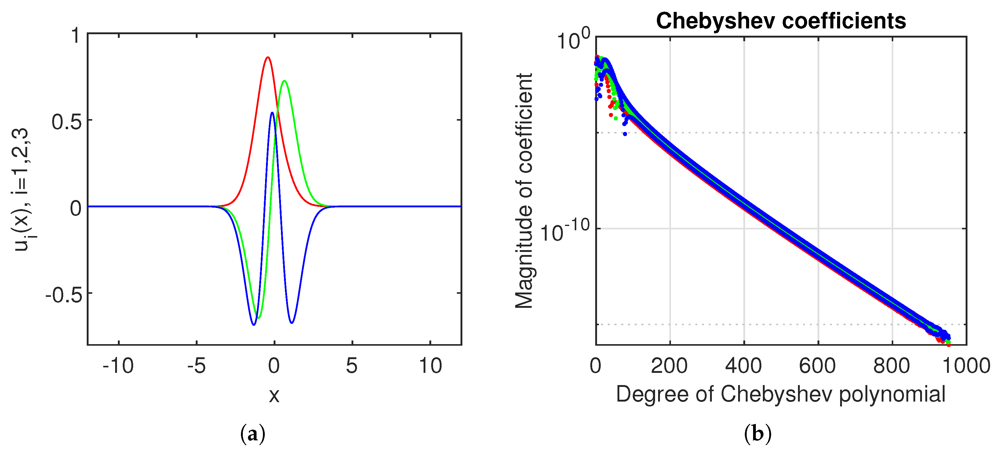
Thus, the first three eigenvectors are shown in Figure 1a. These differ in the number of roots, i.e., $v_i\left(x\right)$ has $i-1$ roots for $i=1, 2, 3$.

Panel (b) in Figure 1 shows for each of the three eigenvectors the following dependence:

$$\left|u_n\right|\simeq e^{-\mu n},\mu \simeq 15/950, n\to N,$$

(5)

which means a better rate compared with that provided by DESCM and displayed in Formula (6).

It can also be seen that this graph is clean, meaning it does not have plateau points. Clearly, this is an exponential convergence of the ChC solution (see [16] for definitions of various types of convergence for spectral methods).

The first six eigenvalues of problem (1) are reported in

Table 1. The first six eigenvalues of problem (1).

Order of Eigenvalue	Eigenvalue
${\lambda }_1$	0.6908884498455730
${\lambda }_2$	4.947137149019847
${\lambda }_3$	9.226710814473009
${\lambda }_4$	14.9839286449549
${\lambda }_5$	21.41731241774201
${\lambda }_6$	28.83976692293931 1

¹ Chebfun worked on the finite interval $[-X,X]$ with $X:=12$.

. The computed value of the first eigenvalue ${\lambda }_1$ coincides up to the sixth decimal with the one reported in [6]. Unfortunately, in this work, there are no more eigenvalues or eigenfunctions reported, so we cannot extend the comparison.

The AAA algorithm is implemented in Chebfun’s aaa or aaax routines.

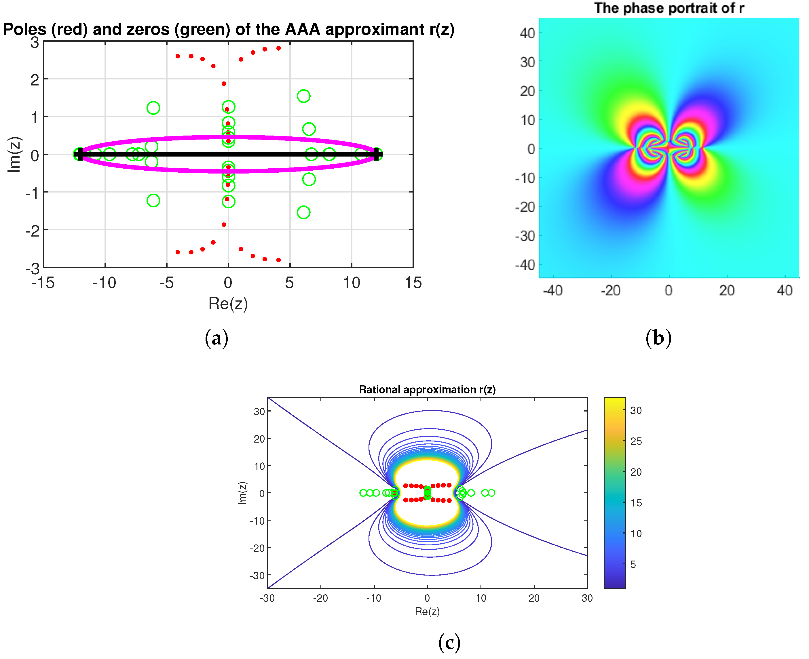
The poles and zeros corresponding to the first eigenvector are depicted in Figure 2a. Only some of them remain purely imaginary, like the poles of problem (1). A two-fold symmetry of the phase portrait is depicted in Figure 2b.

Rational approximations sometimes have poles where one does not expect them, far from any singularities of an analysed function, which may destroy the quality of an approximation at least as measured in the ∞-norm. Fortunately, neither spurious poles nor Froissart doublets have produced our approximation. AAA extrapolation into the complex plane of the first eigenvector to the problem (1) is available in Figure 2c.

From the phase portrait Figure 2b, we observe the colour sequence RedYellowGreenBluePurple, which confirms the zeros (counterclockwise) and the poles (clockwise). From the same phase portrait, it seems that the first eigenvector has stable behaviour at infinity ($arg\left(r\right(z\left)\right)=\pi$ at infinity). Moreover, the flower shape with symmetrical petals indicates a rational function, and eventually, from the distribution of colours, we have the right to believe that there are no other zeros/poles.

For a more subtle interpretation of the phase portraits, we refer to the book [17]. A very useful and instructive analysis can also be found in [11].

A nice feature of this eigenproblem is that all singularities are simple complex poles, leading to a simpler analysis than if we had to consider other singularities, such as branch points.

In [6], the authors observe that a key feature in sinc numerical methods is the distance from the real axis for which the function of interest is analytic. This strip is traditionally denoted by ${\mathcal{D}}_d:=\left\{z\in \mathbb{C}:\left|\mathcal{I}\left(z\right)\right|<d\right\}$ for some $d>0.$ Normally, the larger the value of d, the better sinc numerical methods typically perform.

However, the authors of [6] claim that they successfully solve a singular SL eigenvalue problem by a double exponential sinc collocation method (DESCM). The convergence of the DESCM algorithm is at the rate

$$O\left({\displaystyle \frac{N^{5/2}}{{log}^2\left(N\right)}}e{\displaystyle \frac{-kN}{log\left(N\right)}}\right),$$

(6)

where N refers to the index of the $2N+1$ collocation points.

Thus, by comparing (5) and (6), we can definitely state that the ChC method implemented using Chebfun produces comparable results at a significantly better rate.

Our numerical experiments show that the results obtained with Chebfun are not influenced by the width d of the analyticity strip. Even in this regard, Chebfun outperforms DESCM.

Moreover, we contradict the statement that DESCM yields the best available convergence for problems with end-point singularities or infinite-sized domains. This time, a simple MATLAB code calculates the first eigenvalue that coincides up to the eighth decimal place with ${\lambda }_1$ from Table 1.

2.3. The Accuracy in Computing Eigenvalues (The Relative Drift)

We want to separate the ‘good’ eigenvalues from the ‘bad’ ones, that is, inaccurate eigenvalues. A way to achieve this aim is to compare the eigenvalues computed for different orders of length X. Only those whose difference or resolution-dependent drift is ‘small’ can be believed.

The relative drift of the j-th eigenvalue with respect to the parameter X is defined as follows (see [15]):

$${\delta }_{j,relative,X_1,X_2}:=\left|{\lambda }_j^{X_1}-{\lambda }_j^{X_2}\right|/\left|{\lambda }_j^{X_1}\right|,X_1\ne X_2,$$

(7)

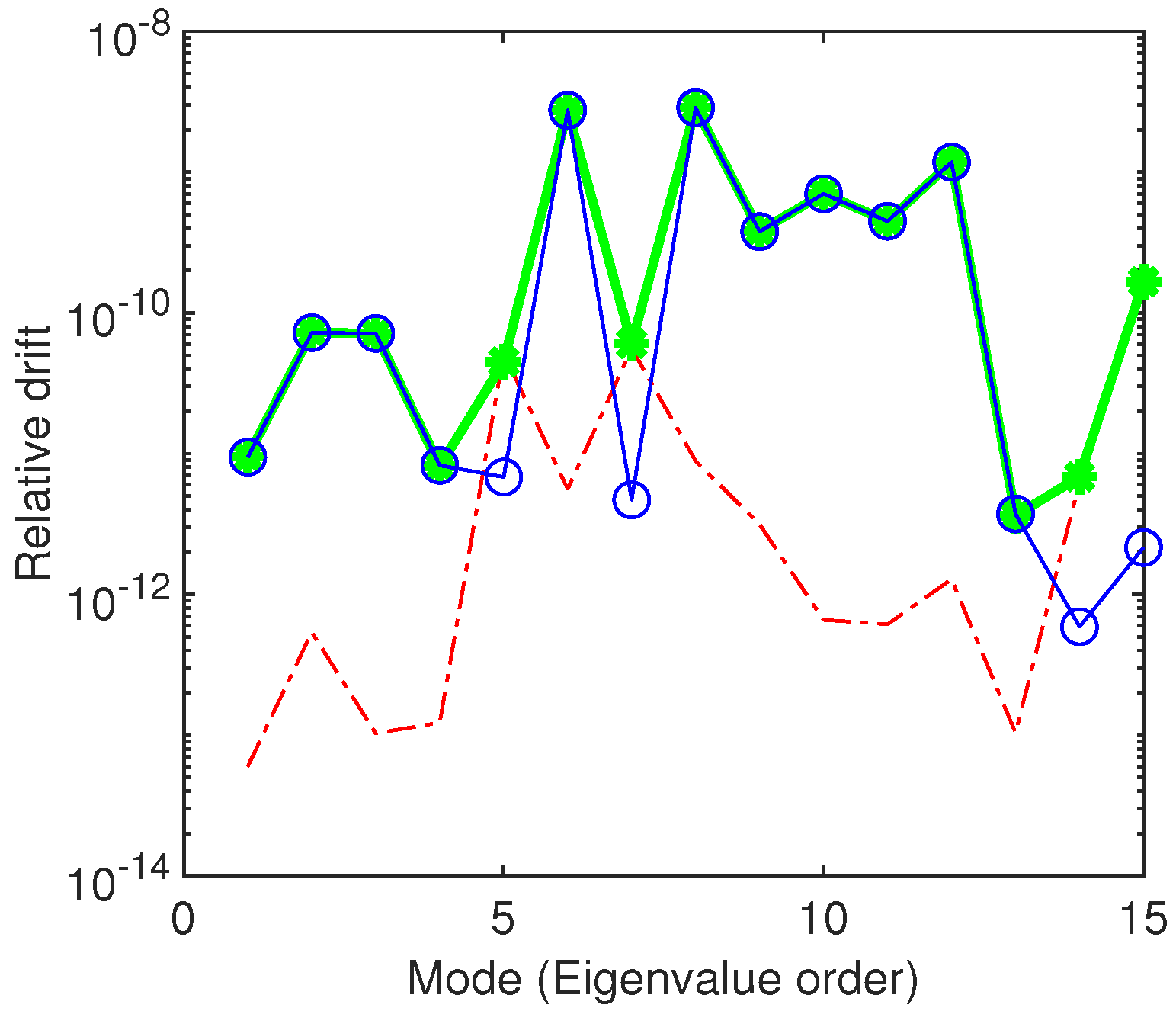
where ${\lambda }_j^X$ is the j-th eigenvalue, after the eigenvalues have been sorted, calculated using a specific value of the parameter X. The dependence of the relative drift for $j=1, 2, \dots , Ne$, where $Ne$ is the number of analysed eigenvalues, on the index (mode) j will be displayed in a log-linear plot.

The results of Figure 3 indicate that the closest eigenvalues, i.e., the most accurate, are obtained when the length X ranges in the interval $[8,12].$ This is especially true for the first four eigenvalues.

To ensure once more that the results obtained are correct, we have solved the eigenvalue problem by the conventional sinc collocation method. We have frequently used this method before the advent of Chebfun, and it is based on the differentiation matrices provided in the seminal paper [18]. The first and only eigenpair produced by this method is in perfect agreement with that obtained through Chebfun.

3. The Complex Singularities of the Thin Film Flow Problem

3.1. The Marangoni and Gravity Effects

Let us consider Equation (2) with nonconvex flux function defined by

$$f\left(h\right):=h^2-h^3,$$

(8)

where the first term represents the Marangoni stress, and the second term represents the gravity stress. To Equation (2), we attach the boundary conditions:

$$h\to h_{\infty },x\to -\infty \mathrm{and}h\to b>0, x\to \infty \mathrm{with}b<h_{\infty }.$$

(9)

We choose boundary conditions consistent with the experiments described in our old paper [19]. Thus, far upstream, i.e., $x\to -\infty$, the film achieves a uniform thickness $h_{\infty }$, determined by a meniscus that forms on the surface of the reservoir. To describe the behaviour of a completely wetting system, we assume the presence of a thin precursor layer of a small thickness, say $b>0$, preceding the leading front of the film. Such a positive parameter b is necessary to avoid the well-known paradox for the case of a moving contact line (see, for instance, [8]). So we get the second boundary condition in (9).

The Chebfun solution to problem (2)–(9) has been computed using the initial data:

$$h\left(x,0\right):={\displaystyle \frac{1}{2}}[\left(h_{\infty }+b\right)+\left(b-h_{\infty }\right)\tanh (x-x_0)],$$

(10)

where we chose $x_0:=-5$.

Unfortunately, as it is formulated, this problem is not well-posed; the order of differentiation is four, and we only have two boundary conditions specified. In order to circumvent this difficulty, we observe that the initial data (10) is compatible with the boundary conditions (9). We differentiate twice the relation (10), and thus we get two supplementary boundary conditions, namely

$$h_{xx}\to h_{xx}(-\infty ,0),x\to -\infty \mathrm{and}{h}_{xx}\to h_{xx}(\infty ,0),x\to \infty .$$

(11)

They are called boundary conditions of type pressure because the curvature of the free surface $h_{xx}$ multiplied by the surface tension $\sigma$ equals the pressure.

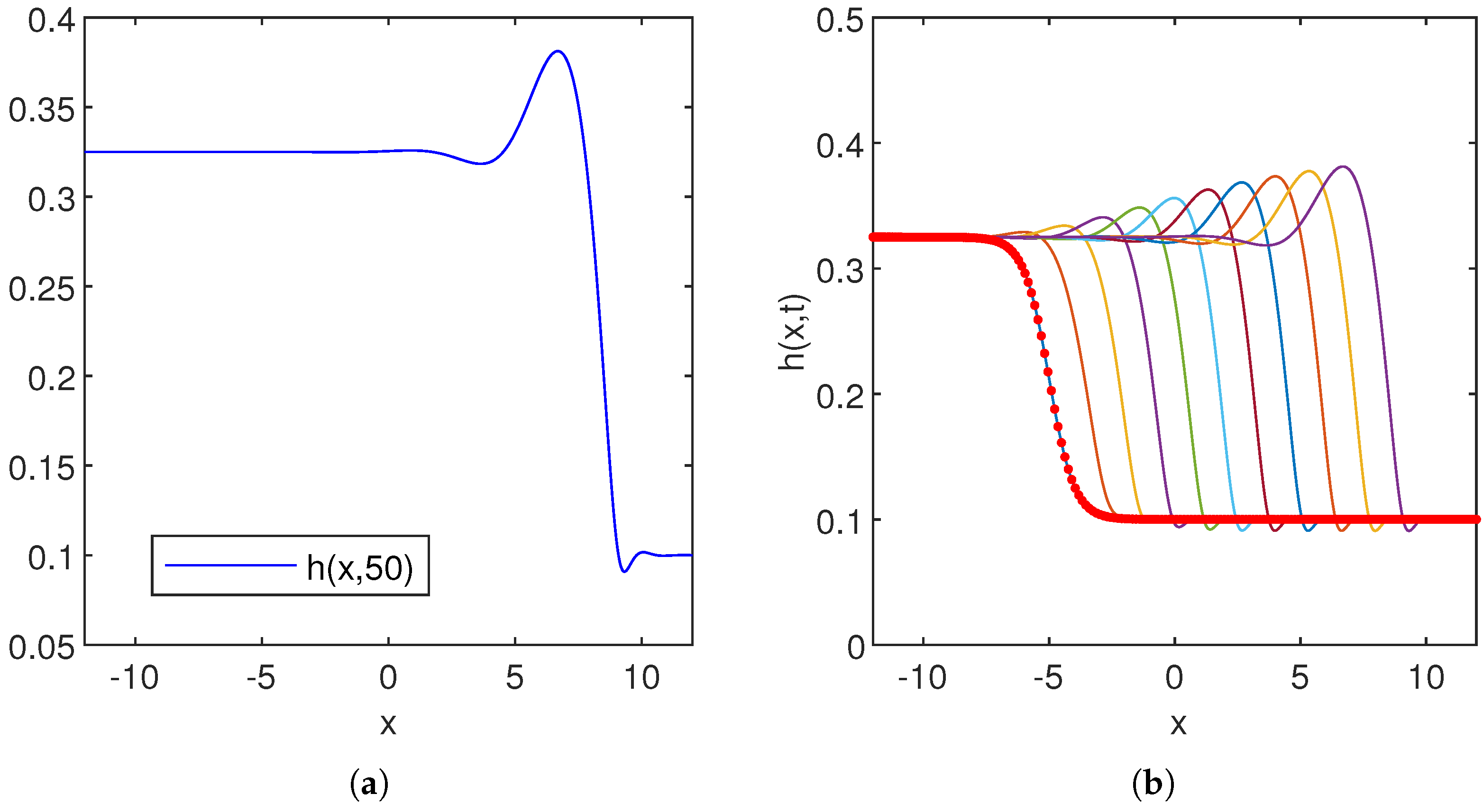
A remark on the initial data is in order at this point. It is well-known by the Cauchy-Kowalevsky theorem (see [20]) that for any holomorphic (analytic) function $h(x,0)$ in a neighbourhood of $x=0$ the Equation (2) has a unique holomorphic solution $h(x,t)$ in a neighbourhood of the origin satisfying (10). Thus, the holomorphic solutions of (2) in a neighbourhood of the origin are completely characterised by the initial data. And this fact is obvious in Figure 4b.

This equation is stiff, and the initial condition matches the boundary conditions perfectly.

To march in time, we used the Chebfun routine pde15s. The routine pde23t works just as well.

For this problem, a very detailed mathematical analysis, including the existence of solutions, their regularity and uniqueness, is provided in [7].

The purpose of our analysis is entirely different, that is, the study of the complex singularities of these problems. However, the numerical results obtained by us (the solution at the final time $t:=50$ and the succession of waves) displayed in the Figure 4 panels (a) and (b) are perfectly similar to those reported in [7], Figure 4 and [9], Figure 2.

To undertake the analysis in the complex plane, we have used the following Chebfun sequence:

Y = linspace(-12,12,200);

 [r,pol,res,zer] = aaa(h(Y,end),Y,’tol’,1.e-5,’lawson’,0);

where $h(Y,end)$ is the Chebfun solution to problem (2)–(9)–(11) at the final moment.

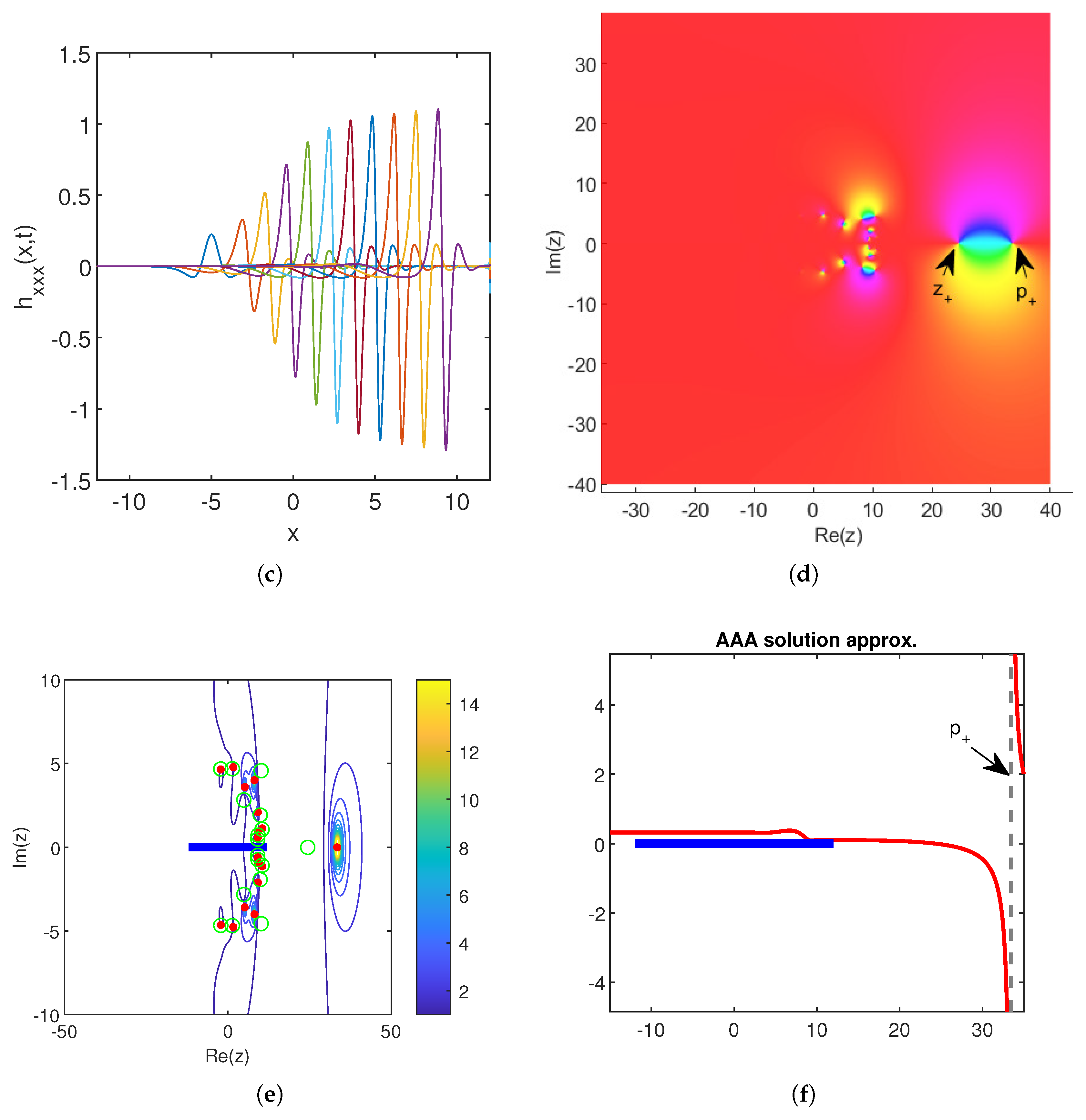
We have obtained 0 Froissart doublets and 17 poles. The only pole of interest is the real one marked with $p_{+}=$$33.47695765330845$. This corresponds to the real zero denoted by $z_{+}=$$24.45953250966801$. Both are marked on panel (d) and have been computed with the residuum $2.588197445394010$.

From the phase portrait (d), we observe that the pole $p_{+}$ and the zero $z_{+}$ are connected by a smooth yellow sector below. The complex pairs of complex poles and zeros on the left are of much less importance.

As can be seen very clearly from Figure 4f, this pole signifies a branch point.

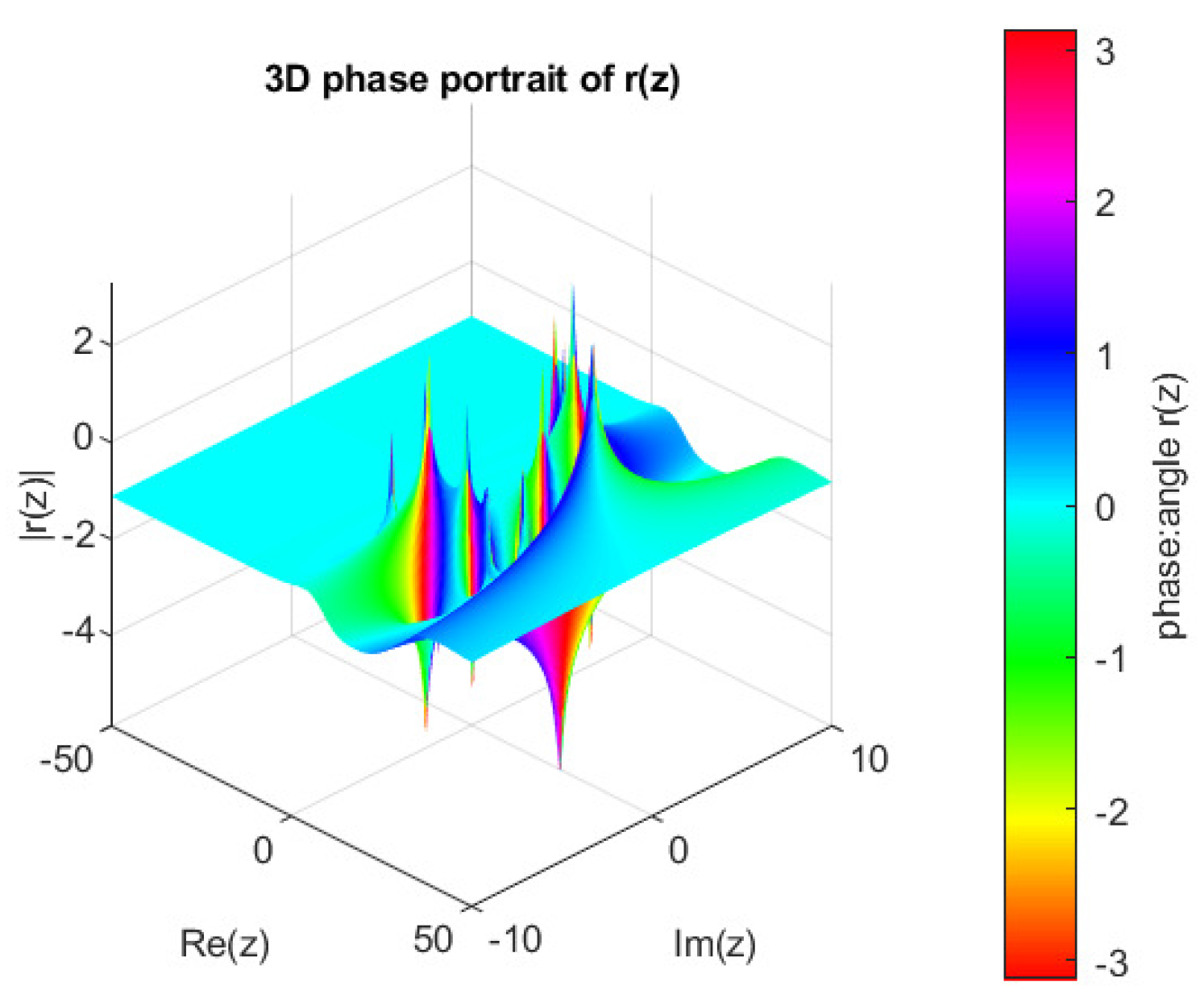
All poles with their importance are visible again in Figure 5.

3.2. Preservation of Solutions Non-Negativity

In our Equation (2), the parabolicity degenerates at $h=0.$ We observe that this is a nonlinear degeneracy in the sense that it depends on the unknown function h rather than on the independent variables x or t. Despite this rather strange behaviour, the numerical solutions which approximate the classical solution of this problem preserve non-negativity, i.e.,

$$h\left(x,t\right)\ge 0\mathrm{for}\mathrm{all}\mathrm{time}t>0\mathrm{if}h\left(x,0\right)\ge 0.$$

(12)

Moreover, as is apparent from the first two panels of Figure 4, the Chebfun solutions preserve positivity, pointwise positivity, and maintain non-shrinking support.

For a simpler equation, namely

$$h_t={\left(h^3{h}_{xxx}\right)}_x,$$

such preserving properties have been rigorously proved (see, for instance, [21]). Unfortunately, no proof for general solutions has been published, as far as we know.

3.3. Capillary Shock Profile

We are now looking for solutions in the form of a capillary shock profile or travelling waves $h(x-st)$ to Equation (2). We have to solve the equation (see [7]):

$$h^3{h}_{xxx}-sh+h^2-h^3-D{h}^3{h}_x-Q=0,$$

(13)

where

$Q:=-b{h}_{\infty }+b^2{h}_{\infty }+h_{\infty }^{2}b$ and $s:=h_{\infty }+b-h_{\infty }^2-h_{\infty }b-b^2$.

Singular and nonlinear third-order equations of this type have been solved using shooting in the paper [22]. Unfortunately, no error analysis can be found in that paper. Instead, using Chebfun for similar problems, we have provided solutions accompanied by a rigorous error analysis in our work [23].

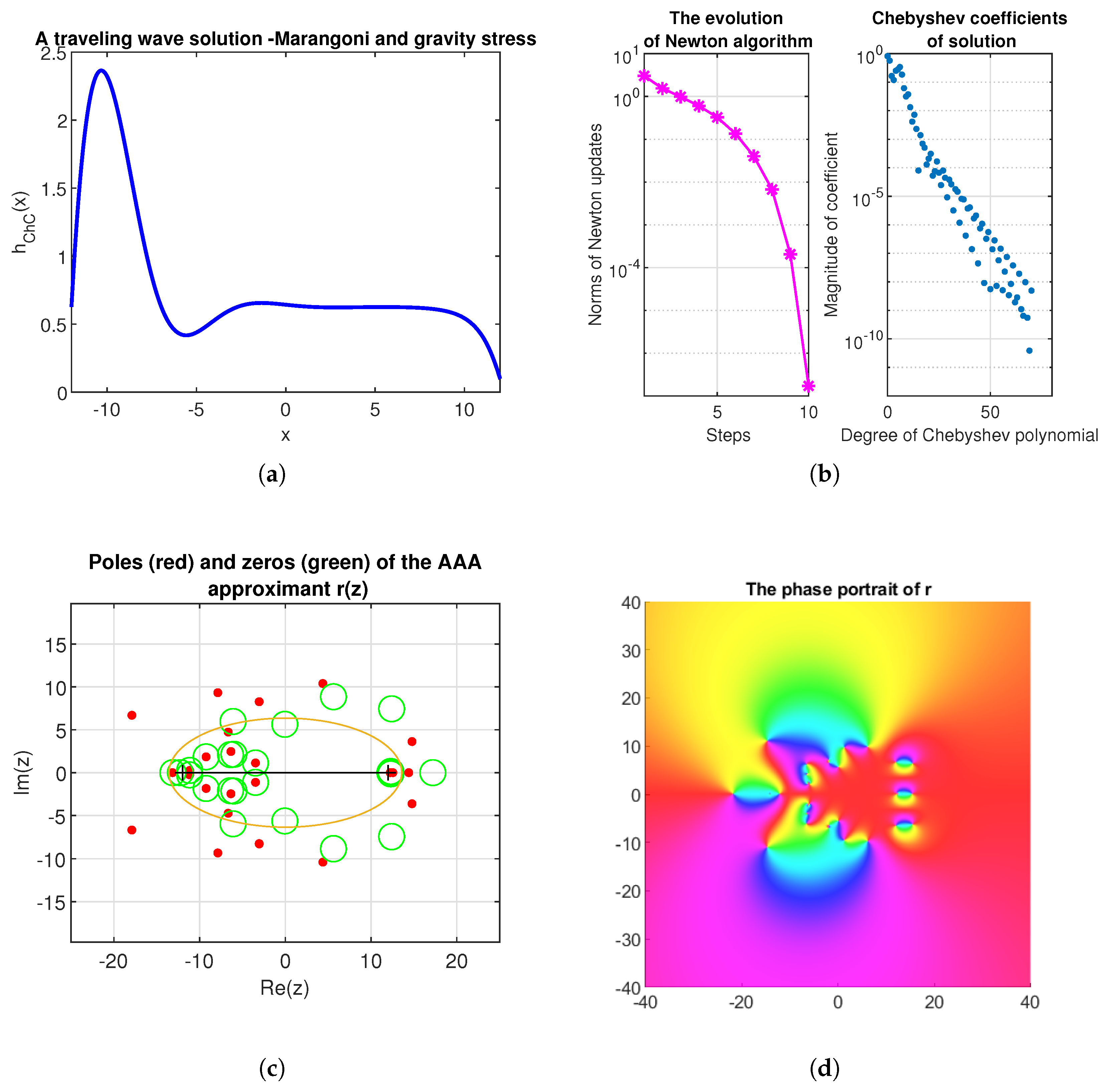
The solution to this problem has been computed by Chebfun with an accuracy of order ${10}^{-11}.$ The length of the solution has been determined by Chebfun to be $N=136$, and it is displayed in panel (a) Figure 6.

Newton’s algorithm for calculating this solution converges in eleven iterations and has an order of about 1.81 (see the left panel in Figure 4b). This order was computed using the paper [24]. From the right panel of the same figure, we can infer that the coefficients $h_n$ of the Chebfun solution decrease according to the asymptotic estimation

$$\left|h_n\right|\simeq e^{-\mu n},\mu \simeq 15/150,n\to N.$$

(14)

Thus, still an exponential rate of convergence is attained by Chebfun, which is better than in the case of the SL problem (1).

In the complex plan, the analysis changes drastically in this third problem.

We have used the following Chebfun sequence:

Y = linspace(-12,12,200);

 [r,pol,res,zer] = aaa(h(Y),Y,’mmax’,25,’lawson’,0);}

where h is the Chebfun solution to problems (13)–(9).

We have obtained 0 Froissart doublets and 24 poles. This Chebfun sequence differs slightly from the one in Section 3.1 with respect to the input parameter mmax vs. tol. Moreover, these sequences, added to a Chebfun code to calculate the solution, analogous to the one presented in our paper [23], are all that is needed to perform this analysis.

As a general observation, we can see from Figure 6c that the poles and zeros are symmetrically placed concerning the x axis. Moreover, the red colour at infinity in the phase portrait signifies $arg\left(r\right(z\left)\right)=0$, that is, a stable behaviour. On the real axis, it is easy to observe zero-pole cancelation (places where zeros and poles are very close, and then they do not appear in the phase portrait with distinct colors). In this situation, the poles are $p_{-}^3$, $p_{-}^4$, $p_{+}^2$, $p_{+}^3$ and $p_{+}^4.$ On the right-hand side, we observe three poles and three zeros that are “nicely connected” by a yellow arc (bottom). Similarly to the left-hand side (negative semiplane), we observe the three poles (one on the real axis, two symmetric with respect to the real axis) and a zero in $[-20,-10]$ that “escapes” from the zero-pole cancellation phenomenon.

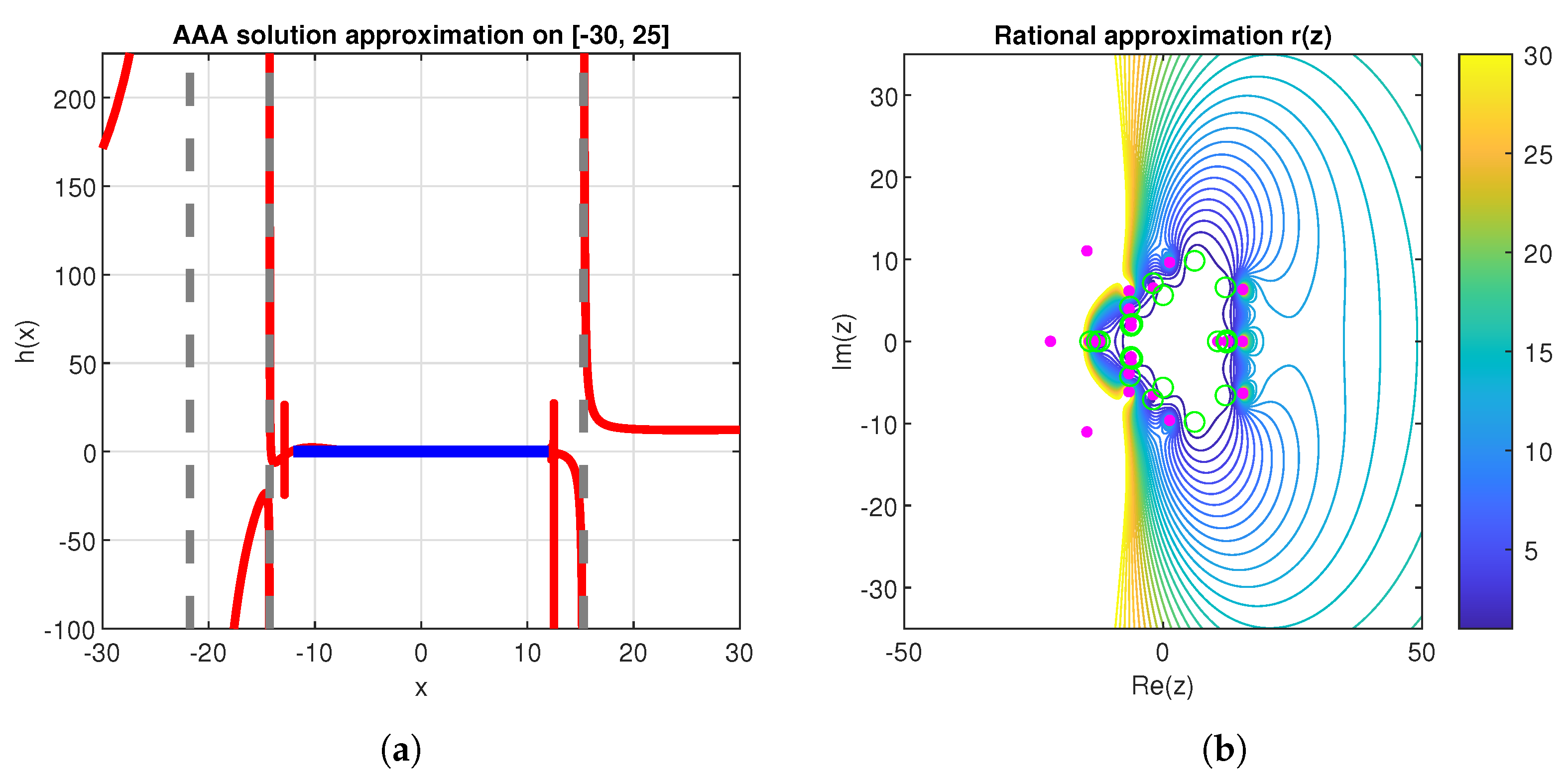
The solution $h\left(x\right)$ of the problem (13)–(9) is not an analytic function on the entire real line, i.e., there are three branch points. The first, where the continuity is broken, is situated at the left pole $p_{-}^2=$$-14.27037925761109$, and the rightmost branch point is situated at the largest positive pole $p_{+}^1=$$15.29228208548559\times 10$. The leftmost pole $p_{-}^1$, is situated at the abscissa $-21.78178506233091$. This situation is numerically illustrated in the left panel (a) of Figure 7. The thick blue line marks the integration domain and does not contain any real poles!

The real poles, along with their residuals and significance in the context of the differential equation, are listed in

Table 2. The real poles, their residuals and an interpretation in connection with Figure 7a.

Poles	Interpretation	Abscissa	Residual
$p_{-}^1$	b p $\alpha$	$-21.78178$	$-8.456699\times {10}^2$
$p_{-}^2$	b p	$-14.27037$	$1.742982$
$p_{-}^3$	s o $\beta$	$-12.86426$	$3.188191\times {10}^{-2}$
$p_{-}^4$	n $\gamma$	$-12.24661$	$-1.947585\times {10}^{-5}$
$p_{+}^1$	b p	$15.29228$	$13.76886$
$p_{+}^2$	s o	$12.49836$	$-6.550628\times {10}^{-2}$
$p_{+}^3$	n	$12.25851$	$4.268247\times {10}^{-3}$
$p_{+}^4$	n	$10.53572$	$-8.307072\times {10}^{-11}$ Λ

^Λ Chebfun worked on the finite interval $[-X,X]$ with $X:=12$. ^$\alpha$ branch point ^$\beta$ solution oscillation ^$\gamma$ neglected.

.

3.4. The Marangoni Effect

We consider as a last example, the Equation (2) with the convex flux function defined only by

$$f\left(h\right):=h^2.$$

(15)

We applied our strategy to this particular case, but from a mathematical point of view, nothing stood out; therefore, we did not consider it worth exposing in more detail.

However, travelling wave solutions will be obtained in this case by solving the nonlinear third-order equation

$$h^3{h}_{xxx}-(1+b)h+h^2+b=0,$$

(16)

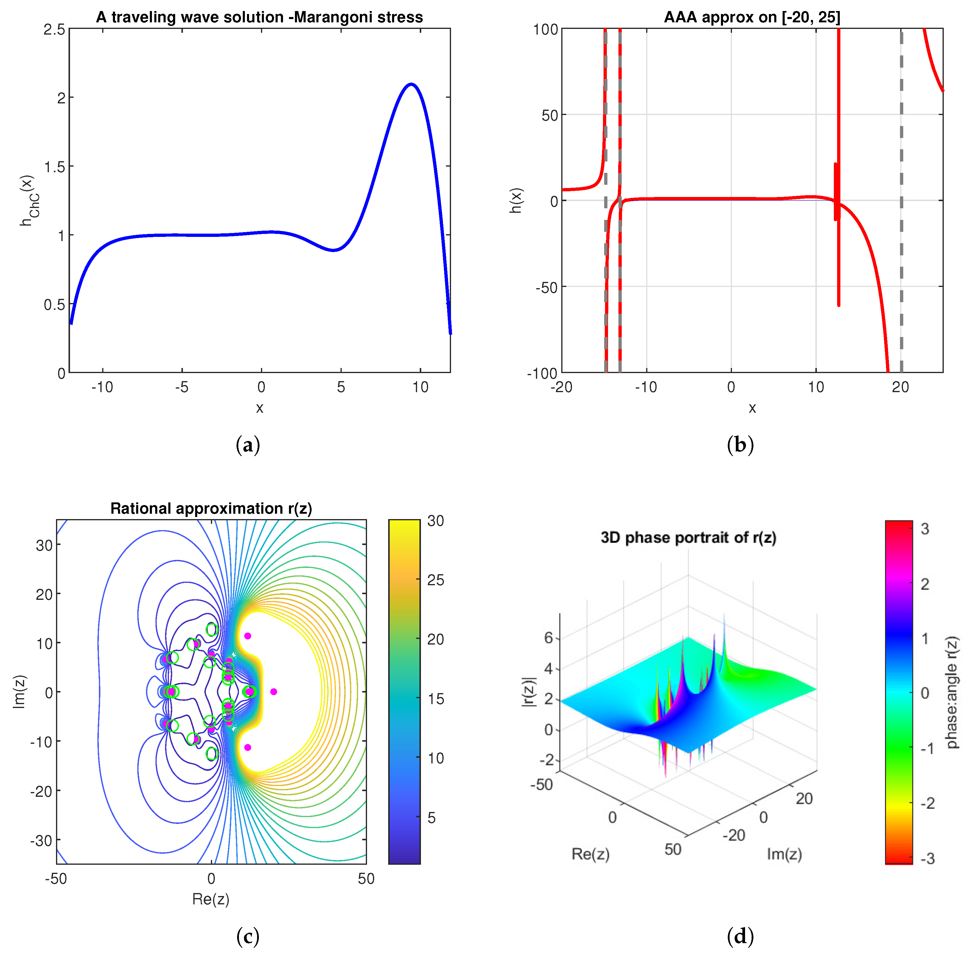
where b is a constant, along with the boundary condition (9). The numerical results are gathered in Figure 8. Apart from these results, we mention that the Chebfun solved length has been $N=231$, the ChC convergence is again exponential, and the order of the Newton method only reached the value $1.60$.

Of the 24 poles generated by the aaa, 6 are real. All are visible in Figure 8b–d. The rightmost one has an abscissa 20.09334166262438 and a residue of order 10², and the leftmost one has an abscissa −14.81960440944722 and the residue equals −5.90. All other residuals are smaller in absolute value.

The same fundamental observation remains valid for the case of exclusively gravitational stress, i.e., $f\left(h\right):=h^3$.

4. Discussion

The emergence of some branch point-type singularities in the study of all the last three problems is an important aspect from both a numerical and an applicative perspective.

We are tempted to formulate a conjecture, namely that the influence of a real pole depends on the size of its residue (see lines 4, 7 and 8 in Table 2) and the discussion in the last Section 3.4.

The existence of simple complex poles, both in this case and in the case of the SL problem (1), does not bring anything significant either numerically and/or from the perspective of differential problems.

The problem (13)–(9) as well as the problem (16)–(9) are both not well-posed; i.e., the order of differentiation is three, and we only have two boundary conditions attached. Chebfun notes this fact, and a warning is issued, namely Operator may not have the correct number of boundary conditions. What is very interesting is that Chebfun successfully solves these problems.

An important observation can be made by reading

Table 3. The errors in the AAA approximation of solutions.

The Problem	Error in $\mathit{inf}$ Norm
(2)–(9)–(11)	$2.58336\times {10}^{-6}$ 1
(13)–(9)	$3.2720\times {10}^{-9}$
(16)–(9)	$9.5562\times {10}^{-11}$

¹ Solution considered at the final moment $t=50$.

. It is clear from it that the accuracy with which the AAA algorithm works decreases with increasing problem complexity, which was expected.

It is also important to note that spurious (false) poles did not affect our analysis. However, in the paper [4], the authors provide a Chebfun code for their elimination (clean).

Of course, there is room for improvement, especially in making a more accurate connection between the size of the residue of a real pole and the type of singularity it implies.

5. Conclusions

Based on the numerical evidence presented here, we appreciate that the used strategy should be considered successful. In tackling ODE and PDE, the singularity dynamics have been tracked accurately.

The phase portrait for a specified solution was used to detect the hidden singularities of a specified solution. In fact, with the proposed strategy, all singularities in the complex plane are taken into account, not just those close to the real axis.

A fundamental result produced by our analysis consists of finding the widest possible intervals on the real axis where the studied problems are well formulated, meaning they avoid singularities of the branch point type.

In other words, the proposed strategy suggests a well-founded path for the truncation of an unbounded domain! For similar two-dimensional domains, an analogous study is in progress.

The present work adds to our series of works [15,23] in which we have attempted to demonstrate the superiority of the ChC implemented through Chebfun over shooting-type methods in solving nonlinear and even singular BVPs.

References

1. Boyd, J.P. The Blasius Function in the Complex Plane. Exp. Math. 1999, 8, 381–394. [Google Scholar] [CrossRef]
2. Caflisch, R.E.; Gargano, F.; Sammartino, M.; Sciacca, V. Complex singularities and PDEs. Riv. Mat. Univ. Parma 2015, 6, 69–133. [Google Scholar]
3. Viswanath, D.; Şahutoğlu, S. Complex Singularities and the Lorenz Attractor. SIAM Rev. 2010, 52, 294–314. [Google Scholar] [CrossRef]
4. Trefethen, L.N. Numerical analytic continuation. Japan J. Appl. Math. 2023, 40, 1587–1636. [Google Scholar] [CrossRef]
5. Nakatsukasa, Y.; Sète, O.; Trefethen, L.N. The AAA algorithm for rational approximation. SIAM J. Sci. Comput. 2018, 40, A1494–A1522. [Google Scholar] [CrossRef]
6. Gaudreau, P.; Slevinsky, R.; Safouhi, H. The double exponential sinc collocation method for singular Sturm-Liouville problems. J. Math. Phys. 2016, 57, 043505. [Google Scholar] [CrossRef]
7. Bertozzi, A.L.; Münch, A.; Shearer, M. Undercompressive shocks in thin film flows. Physica D 1999, 134, 431–464. [Google Scholar] [CrossRef]
8. Buckingham, R.; Shearer, A.; Bertozzi, A. Thin Film Travelling Waves and the Navier Slip Condition. SIAM J. Appl. Math. 2003, 63, 722–744. [Google Scholar] [CrossRef]
9. Münch, A. Shock transitions in Marangoni gravity-driven thin-film flow. Nonlinearity 2000, 13, 731–746. [Google Scholar] [CrossRef]
10. Weideman, J.A.C. Computing the Dynamics of Complex Singularities of Nonlinear PDEs. SIAM J. Appl. Dyn. Syst. 2003, 2, 171–186. [Google Scholar] [CrossRef]
11. VandenHeuvel, D.J.; Lustri, C.J.; King, J.R.; Turner, I.W.; McCue, S.W. Burgers’ Equation in the Complex Plane. Numer. Algorithms 2022, 90, 1305–1326. [Google Scholar]
12. Trefethen, L.N. Approximation Theory and Approximation Practice, Extended Edition; SIAM: Philadelphia, PA, USA, 2019; pp. 251–263. [Google Scholar]
13. Trefethen, L.N. Quantifying the ill-conditioning of analytic continuation. BIT Numer. Math. 2020, 60, 901–915. [Google Scholar] [CrossRef]
14. Driscoll, T.A.; Hale, N.; Trefethen, L.N. (Eds.) Chebfun Guide; Pafnuty Publications: Oxford, UK, 2014; Available online: www.chebfun.org (accessed on 1 January 2020).
15. Gheorghiu, C.-I. Accurate Spectral Collocation Computation of High-Order Eigenvalues for Singular Schrödinger Equations. Computation 2021, 9, 2. [Google Scholar] [CrossRef]
16. Aurentz, J.L.; Trefethen, L.N. Chopping a Chebyshev series. ACM Trans. Math. Softw. 2017, 43, 33. [Google Scholar] [CrossRef]
17. Wegert, E. Visual Complex Functions. An Introduction with Phase Portraits; Springer: Basel/Heidelberg, Germany; New York, NY, USA; Dordrecht, The Netherlands; London, UK, 2012. [Google Scholar]
18. Weideman, J.A.C.; Reddy, S.C. A MATLAB Differentiation Matrix Suite. ACM T. Math. Softw. 2000, 26, 465–519. [Google Scholar] [CrossRef]
19. Chifu, E.; Gheorghiu, C.I.; Stan, I. Surface Mobility of Surfactant Solutions XI. Numerical Analysis for the Marangoni and Gravity Flow in a Thin Liquid Layer of Triangular Section. Rev. Roum. Chim. 1984, 29, 31–42. [Google Scholar]
20. Tahara, H. On the Singularities of Solutions of Nonlinear Partial Differential Equations in the Complex Plane. RIMS Kôkyûroku 2004, 1397, 102–111. [Google Scholar]
21. Bernis, F. Viscous flows, fourth-order nonlinear degenerate parabolic equations and singular elliptic problems. In Free Boundary Problems: Theory and Applications; Diaz, J.I., Herrero, M.A., Linan, A., Vazquez, J.L., Eds.; Pitman Research Notes in Mathematics 323; Longman: Harlow, UK, 1995; pp. 40–56. [Google Scholar]
22. Tuck, E.O.; Schwartz, L.W. A Numerical and Asymptotic Study of some Third-Order Ordinary Differential Equations Relevant to Draining and Coating Flows. SIAM Rev. 1990, 32, 453–469. [Google Scholar] [CrossRef]
23. Gheorghiu, C.-I. Chebyshev Collocation Solutions to Some Nonlinear and Singular Third-Order Problems Relevant to Thin-Film Flows. Mod. Math. Phys. 2025, 1, 5. [Google Scholar] [CrossRef]
24. Cătinaş, E. How Many Steps Still Left to x*? SIAM Rev. 2021, 63, 585–624. [Google Scholar] [CrossRef]
Figure 1. Chebfun working on the domain [ 12 , 12 ] produced the following outcomes: (a) The first three eigenvectors of the problem (1), in order, are red, green and blue. (b) The Chebyshev coefficients of the first three eigenvectors. They decrease linearly and overlap on a log-linear plot.
Foundations 06 00004 g001
Figure 2. Chebfun working on [ 12 , 12 ] produced the following outcomes concerning problem (1): (a) Poles (red dots), zeros (green circles) and Bernstein ellipse for the first eigenvector. (b) Phase (argument) portrait of the approximation r ( z ) to the first eigenvector of the problem (1). (c) Rational approximation of r ( z ) . Contour plots of rational approximants to the numerical first eigenvector, in the complex plane.
Foundations 06 00004 g002
Figure 3. The relative drift of the first fifteen eigenvalues to the problem (1); red dotted line refers to X 1 : = 12 , X 2 : = 8 , green circled line refers to X 1 : = 12 , X 2 : = 8 , and blue circled line refers to X 1 : = 12 , X 2 : = 15 .
Foundations 06 00004 g003
Figure 4. Chebfun working on [ 12 , 12 ] with D : = 0.1 , h : = 0.325 and b : = 0.1 produced the following outcomes: (a) The solution to the problem (2)–(9)–(11), starting from the initial data (10). (b) The solution at moments t = [ 0 : 5 : 50 ] . (c) The third derivative of the solution at the same time moments. This is sharp but still bounded. (d) The phase portrait corresponds to the solution at the final moment. (e) The absolute value | h ( z , 50 ) | of the AAA extrapolation into the complex plane of the solution is plotted. The poles are marked by red dots, and the zeros are marked with green circles. (f) Extension of the solution on the real axis with pole p + as a branch point is displayed. The domain of integration is marked by a thick blue line.
Foundations 06 00004 g004aFoundations 06 00004 g004b
Figure 5. The 3D phase portrait of r ( z ) .
Foundations 06 00004 g005
Figure 6. Chebfun working on [ 12 , 12 ] with D : = 0.1 , h : = 0.325 and b : = 0.1 produced the following outcomes: (a) The traveling wave solution to the problem (13)–(9) when Marangoni and gravitational stresses compete. (b) Evolution of Newton’s algorithm left panel, and the behaviour of Chebyshev coefficients of the solution, right panel. Again, no plateau point is found. (c) Poles (red colour), zeros (green colour) and the Bernstein ellipse are depicted. (d) The phase (argument) portrait corresponding to the travelling wave solution.
Foundations 06 00004 g006
Figure 7. Chebfun working on [ 12 , 12 ] with D : = 0.1 , h : = 0.627 and b : = 0.1 produced the following outcomes: (a) The AAA approximation of the solution with three branch points at real poles p 1 , p 2 and p + 1 marked by dotted lines (see Table 2). The solution plotted in panel (a) of the previous figure overlaps the blue line due to the scale on the ordinate axis. (b) The rational approximation of the solution is symmetric with respect to the x axis. The magenta dots represent poles, and the green circles represent zeros.
Foundations 06 00004 g007
Figure 8. Chebfun working on [ 12 , 12 ] with D : = 0 , h : = 0.325 and b : = 0.1 produced the following outcomes: (a) The solution to the problem (16)–(9), starting from a constant initial data. (b) The extension of the solution on the real axis with singularities at the real poles. (c) The rational approximation around the poles is marked by real dots. (d) The 3 D phase portrait.
Foundations 06 00004 g008