Complexity Assessments for Decidable Fragments of Set Theory. IV: A Quadratic Reduction from Constraints over Nested Sets to Boolean Formulae

Abstract

As a contribution to automated set-theoretic inferencing, a translation is proposed of conjunctions of literals of the forms $x=y\setminus z$, $x\ne y\setminus z$, and $z=\left\{x\right\}$, where $x,y,z$ stand for variables ranging over the von Neumann universe of sets, into quantifier-free Boolean formulae of a rather simple conjunctive normal form. The formulae in the target language involve variables ranging over a Boolean ring of sets, along with a difference operator and relators designating equality, non-disjointness, and inclusion. Moreover, the result of each translation is a conjunction of literals of the forms $x=y\setminus z$ and $x\ne y\setminus z$ and of implications whose antecedents are isolated literals and whose consequents are either inclusions (strict or non-strict) between variables, or equalities between variables. Besides reflecting a simple and natural semantics, which ensures satisfiability preservation, the proposed translation has quadratic algorithmic time complexity and bridges two languages, both of which are known to have an $\mathsf{NP}$-complete satisfiability problem.

1. Introduction

As reported in the survey paper [1], the line of investigation to which this paper belongs began in 1978 (ref. [2]), driven by the goal of developing an automated system for proof-checking and program correctness verification. Since then, identifying decidable fragments of set theory has been regarded as a key step toward achieving that goal. As a matter of fact, in the organization of the proof-checker $\mathsf{Referee/\AE tnaNova}$, which came into existence some thirty years later (ref. [3]), a satisfiability decision tester for a specific class of unquantified set-theoretic formulae plays a central and pervasive role.

When it comes to implementations, complexity emerges as an inescapable issue; this is why we recently undertook a systematic study on the algorithmic complexities of satisfiability testers (see, e.g., [4,5]). In the same frame of mind, this paper enhances a quadratic-cost method (announced ref. [4] and then presented in D. Cantone, A. De Domenico, P. Maugeri, and E.G. Omodeo; a quadratic reduction of constraints over nested sets to purely Boolean formulae in CNF; in Proc. 35th Italian Conference on Computational Logic, volume 2710 of CEUR Workshop Proceedings, pages 214–230. 2020). This translates the formulae of an unquantified language involving set-theoretic variables, Boolean operators, and membership and equality relators into propositional combinations of purely Boolean literals.

The enhancement lies in the availability of a singleton-formation operator ‘{■}’, which increases the expressive power of the source language without affecting the algorithmic time complexity of the translation process; however, the fact that the translation preserves satisfiability as well as unsatisfiability must be proved anew and differently. The material that follows bridges two complexity taxonomies, developed and analyzed in the respective papers [4,5]. These taxonomies, one of which—unlike the other—involves membership, concern fragments of set theory for which satisfiability is decidable.

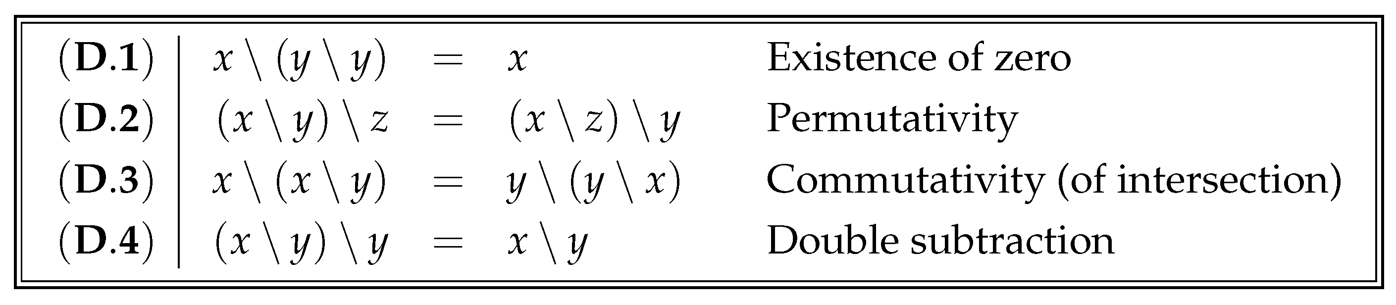
A fit theoretical framework for the study of our target language is the theory of Boolean rings, a merely equational first-order theory endowed with finitely many axioms—at times, one blends this theory with an arithmetic of cardinals (see, e.g., [6])—or just a surrogate of it, cf. Figure 1 in Section 7. Frameworks for the study of the source language are such all-embracing theories as ZF and NBG (the Zermelo–Fraenkel and von Neumann–Bernays–Gödel theories), within which one can cast the whole corpus of mathematical disciplines. Boolean algebra is decidable in its entirety (cf. Section 3.7 ref. [7]); ZF is essentially undecidable, yet nonetheless an effort to find practical decision algorithms for fragments of it began in 1979. The rationale of this long-standing research is that satisfiability testers embodying some knowledge about ZF can act as key inference mechanisms within a programmed system apt to verifying the correctness of large-scale mathematical proofs as envisaged ref. [3].

A priori, one would expect the distance between the performances of decision algorithms for fragments of Boolean algebra, and of the seemingly much more expressive languages whose dictionaries embody nested membership, to be abysmal. Luckily, though, as we will see, this is not the case.

We introduce in Section 2 an interpreted formal language, dubbed $\mathbb{BST}$, within which one can formulate unquantified Boolean constraints. Despite its syntax being quite minimal—$\mathbb{BST}$ only encompasses conjunctions of primitive literals of two forms, namely, $x=y\setminus z$ and $x\ne y\setminus z$ —, the satisfiability problem for $\mathbb{BST}$ is $\mathsf{NP}$-complete (ref. [4]). By way of abbreviations, a number of additional constraints (e.g., literals of the form $x\ne y\cup z$) can be expressed in $\mathbb{BST}$.

Alongside $\mathbb{BST}$, we also consider its natural Boolean closure ${\mathbb{BST}}^{+}$, defined as the language of all propositional combinations—using ∧, ∨, ⟶, ⟷, and ¬ with arbitrary nesting—of atoms of the form $x=y\setminus z$. It is straightforward to verify that the satisfiability problem for ${\mathbb{BST}}^{+}$ can be reduced to that for $\mathbb{BST}$ in nondeterministic polynomial time; therefore, it is $\mathsf{NP}$-complete in turn.

According to our semantics, the domain of discourse to which $\mathbb{BST}$ (and ${\mathbb{BST}}^{+}$) refers is a universe of nested sets; however, as will be seen in Section 5, every satisfiable propositional combination of $\mathbb{BST}$ literals (in particular, every satisfiable $\mathbb{BST}$ constraint) admits a model consisting of sets which are, in a certain sense, ‘flat’. This makes it clear that there is no straightforward way of expressing membership atoms $x\in y$ in $\mathbb{BST}$. Yet, many natural set-theoretic constructors (most notably the singleton operator {■}) inherently interact with membership, and understanding whether and how such constructs can be eliminated while preserving satisfiability and complexity is the main motivation of this paper.

To address this research gap, Section 3 introduces a complexity-aware notion of expressibility, which requires not only a semantic reduction but also an explicit bound on the cost of the translation. While related notions already appear ref. [4], the present formulation is tailored to our setting and is a valuable technical tool that enables the complexity-preservation arguments developed here.

In terms of this notion, Section 6 provides an explicit translation of conjunctions of literals of the three forms $x=y\setminus z$, $x\ne y\setminus z$, and $z=\left\{x\right\}$ into propositional combinations of $\mathbb{BST}$ literals, i.e., into ${\mathbb{BST}}^{+}$. As shown in Section 6.3 and Section 6.4, the translation preserves satisfiability. It yields a conjunction whose conjuncts are either $\mathbb{BST}$ literals or simple disjunctions. Moreover, the translation can be computed in quadratic time (see Section 6.1), which entails that satisfiability remains $\mathsf{NP}$-complete when the singleton operator {■} is added to the constructs of $\mathbb{BST}$. This $\mathsf{NP}$-completeness result was already known (see, e.g., [8]), but our approach derives it anew via an explicit, complexity-controlled elimination procedure.

The concluding section, Section 7, recapitulates what has been accomplished, indicates what we intend to pursue next, and situates our line of investigation in relation to that of other scholars.

2. The Theories $\mathbb{BST}$ and ${\mathbb{BST}}^{+}$

Boolean set theory ($\mathbb{BST}$) is the quantifier-free theory consisting of all finite conjunctions of literals of the forms

$$x=y\setminus z,x\ne y\setminus z,$$

(1)

where x, y, and z are set variables, ranging over the universe of well-founded sets.

Remark 1. 

Throughout, we use the term theory in a nonstandard sense, referring to a collection of set-theoretic formulae—possibly involving, along with primitive symbols, some derived constructs—rather than a deductively closed collection of sentences.

Semantics for the theory $\mathbb{BST}$ is defined in terms of set assignments. Specifically, given a (finite) collection V of set variables, a set assignment M over V—the domain of definition of M, denoted by $\mathsf{dom}\left(M\right)$—is any map from V into the von Neumann universe $\mathcal{V}$ (see below). (Note that our semantics of $\mathbb{BST}$ does not rely on flat sets of urelements (as would be doable). Working with those would call for minor adjustments, unjustified—and perhaps disturbing—in the economy of this paper.) The support of M, denoted by $\mathsf{supp}\left(M\right)$, is the union of the sets assigned by M to the variables in its domain, namely,

$$\mathsf{supp}\left(M\right):=\bigcup _{x\in \mathsf{dom}\left(M\right)}Mx.$$

We shall refer to the cardinality of the support of M as the cardinality of the assignment M. A set assignment M is said to satisfy, or to model, a given literal $x=y\setminus z$, with $x,y,z\in \mathsf{dom}\left(M\right)$, if $Mx=My\setminus Mz$ holds, where ‘∖’ denotes standard set difference. Likewise, M is said to satisfy the literal $x\ne y\setminus z$ if $Mx\ne My\setminus Mz$ holds. Finally, M satisfies a $\mathbb{BST}$-conjunction $\phi$ such that $\mathit{Vars}\left(\phi \right)\subseteq \mathsf{dom}\left(M\right)$ (where $\mathit{Vars}\left(\phi \right)$ denotes the collection of the variables occurring free in $\phi$) if it satisfies all of the conjuncts of $\phi$, in which case we say that M is a model of $\phi$ and write

$$M\vDash \phi$$

(a short for $M{\vDash }_{\mathcal{V}}\phi$). A $\mathbb{BST}$-conjunction $\phi$ is said to be satisfiable if it has some model; otherwise, it is said to be unsatisfiable. It is said to be valid if it is true in every model, in which case we write

$$\vDash \phi$$

(again, a short for ${\vDash }_{\mathcal{V}}\phi$). Two $\mathbb{BST}$-conjunctions $\phi$ and $\psi$ are said to be equisatisfiable if either both are satisfiable or both are unsatisfiable—that is, if $\phi$ has a model if and only if $\psi$ has a model. Equisatisfiability does not require the two formulae to have the same models, but only that they agree in satisfiability, irrespective of their models. The notions introduced in this paragraph, here tailored to the case of $\mathbb{BST}$-conjunctions, extend naturally to all theories discussed in the sequel.

In ref. [4], it is proved that the satisfiability problem for $\mathbb{BST}$, namely, the problem of establishing algorithmically the satisfiability status of any given $\mathbb{BST}$-conjunction, is $\mathsf{NP}$-complete.

• The extension ${\mathbb{BST}}^{+}$.

Recall that $\mathbb{BST}$ only allows for conjunctions of its primitive literals—in particular, a $\mathbb{BST}$-formula is a finite conjunction of constraints of the form $x=y\setminus z$ and $x\ne y\setminus z$. In contrast, ${\mathbb{BST}}^{+}$ is the Boolean closure of $\mathbb{BST}$: it consists of all propositional combinations of atoms of the form $x=y\setminus z$, obtained by unrestrained use of the logical connectives ∧, ∨, ⟶, ⟷, and ¬. Thus, ${\mathbb{BST}}^{+}$ strictly extends $\mathbb{BST}$ by allowing for arbitrary Boolean structure (e.g., disjunctions, implications, and negations at any depth), whereas $\mathbb{BST}$ is restricted to conjunctive constraints.

The satisfiability problem for ${\mathbb{BST}}^{+}$ reduces to that for $\mathbb{BST}$ in nondeterministic polynomial time (by guessing a satisfying assignment for the Boolean structure and checking the resulting conjunction), and hence the satisfiability problem for ${\mathbb{BST}}^{+}$ is $\mathsf{NP}$-complete as well.

The von Neumann Universe

We recall that the von Neumann universe $\mathcal{V}$ of (well-founded) sets, also dubbed von Neumann cumulative hierarchy, is built up through a transfinite sequence of steps as the union $\mathcal{V}:={\cup }_{\alpha \in \mathit{On}}{\mathcal{V}}_{\alpha }$ of the levels ${\mathcal{V}}_{\alpha }:={\cup }_{\beta <\alpha }\mathcal{P}\left({\mathcal{V}}_{\beta }\right)$, with $\mathcal{P}(■)$ denoting the powerset operator and $\alpha$ ranging over the class $\mathit{On}$ of all ordinals.

It can easily be seen that, for every ordinal $\alpha$ (and, in particular, for every integer), we have

$${\mathcal{V}}_{\alpha +1}=\mathcal{P}\left({\mathcal{V}}_{\alpha }\right),$$

and consequently

$$\left|{\mathcal{V}}_{\alpha +1}\right|=2^{\left|{\mathcal{V}}_{\alpha }\right|},$$

(2)

so that $\left|{\mathcal{V}}_{\alpha }\right|<\left|{\mathcal{V}}_{\alpha +1}\right|$.

Based on the level of first appearance in the von Neumann hierarchy, one can define the rank of any set s, denoted $\mathsf{rk}\left(s\right)$. Specifically, $\mathsf{rk}\left(s\right)$ is the ordinal $\alpha$ such that $s\in {\mathcal{V}}_{\alpha +1}\setminus {\mathcal{V}}_{\alpha }$. Hence, for every $\alpha \in \mathit{On}$, the set ${\mathcal{V}}_{\alpha +1}\setminus {\mathcal{V}}_{\alpha }$, hereinafter denoted ${\mathcal{W}}_{\alpha }^{\#}$, collects all sets having rank $\alpha$.

The following lower bound on the number of well-founded sets of any positive integer rank n, to be proved as Proposition A2 in Appendix A, will be useful:

$$\left|{\mathcal{W}}_n^{\#}\right|⩾2^{n-1}.$$

(3)

A particularly important subclass of $\mathcal{V}$ is that of hereditarily finite sets, denoted by $\mathsf{HF}$. By definition,

$$\mathsf{HF}:=\bigcup _{n\in \mathbb{N}}{\mathcal{V}}_n,$$

that is, $\mathsf{HF}$ consists of all sets of finite rank.

Some handy properties of the rank function that we shall tacitly use are the following, which hold for all sets $s,t\in \mathcal{V}$:

• If $s\in t$, then $\mathsf{rk}\left(s\right)<\mathsf{rk}\left(t\right)$;
• If $s\subseteq t$, then $\mathsf{rk}\left(s\right)⩽\mathsf{rk}\left(t\right)$;
• $\mathsf{rk}\left(s\right)=\left\{\begin{array}{cc}0\hfill & \mathrm{if}s=⌀,\hfill \\ {sup}_{u\in s}\left(\mathsf{rk}\left(u\right)+1\right)\hfill & (\mathrm{i.e.,} {\cup }_{u\in s}\left(\mathsf{rk}\left(u\right)+1\right))\mathrm{otherwise}.\hfill \end{array}\right.$

We also recall that well-foundedness, as enforced by the regularity (or foundation) axiom of set theory, precludes the formation of infinite descending membership chains of the form

$$\cdots \in s_2\in s_1\in s_0,$$

and, in particular, membership cycles of the form

$$s_0\in s_n\in \cdots \in s_2\in s_1\in s_0,$$

for any sets $s_i$.

3. From Existential Expressibility to $\mathcal{O}\left(\mathit{f}\right)$-Expressibility Across Theories

We first recall the definition of existential expressibility (cf. [4] for several applications of this notion).

Definition 1 

(Existential expressibility). A formula $\psi \left(x\right)$ is said to be existentially expressible in a theory $\mathcal{T}$ if there exists a $\mathcal{T}$-formula $\mathrm{\Psi }(x,z)$ such that

$$\vDash \mathrm{\Psi }\left({\displaystyle x}\right)⟷(\exists {\displaystyle z})\mathrm{\Psi }({\displaystyle x},{\displaystyle z}),$$

where $x$ and $z$ stand for tuples of set variables.

In spite of the parsimony of $\mathbb{BST}$ as just presented, it turns out (see [4]) that several other Boolean constructs, such as the ones in the list of literals

$$\begin{array}{c}x=⌀,x\subseteq y,x=y\cap z,x=y\cup z,\phantom{\neg }\mathrm{D}\mathrm{ISJ}(x,y),x⊊y,\hfill \\ x\ne ⌀,x⊈y,x\ne y\cap z,x\ne y\cup z,\neg \mathrm{D}\mathrm{ISJ}(x,y),\hfill \end{array}$$

(4)

can be expressed existentially in $\mathbb{BST}$, where $\mathrm{D}\mathrm{ISJ}(a,b)$ is a short for $a\cap b=⌀$.

Ref. [4], existential expressibility was generalized into $\mathcal{O}\left(f\right)$-expressibility (we use standard asymptotic notations $\mathcal{O}(·)$, $\mathrm{\Omega }(·)$, and $\mathrm{\Theta }(·)$ throughout the paper; see, e.g., Ch. 3 of [9]), a notion that helped develop a fine-grained complexity taxonomy of the subfragments of $\mathbb{BST}$.

Definition 2 

($\mathcal{O}\left(f\right)$-expressibility). Let $\mathcal{T}$ be a theory and let $f:\mathbb{N}\to \mathbb{N}$ be a complexity function. A formula $\psi \left(x\right)$—typically involving a construct one aims to eliminate—is said to be $\mathcal{O}\left(f\right)$-expressible in $\mathcal{T}$ if there exists a transformation

$$\phi \left({\displaystyle y}\right)\mapsto {\mathrm{\Psi }}_{\phi }({\displaystyle x},{\displaystyle y},{\displaystyle z})$$

(5)

from $\mathcal{T}$ to $\mathcal{T}$, where no variable in $z$ occurs in $x$ or $y$, such that, for every φ, the following conditions hold:

(a)

The transformation (5) can be computed in $\mathcal{O}\left(f\left(\left|\phi \right|\right)\right)$-time;

(b)

If $\phi \left(y\right)\wedge (\exists z){\mathrm{\Psi }}_{\phi }(x,y,z)$ is satisfiable, then $\phi \left(y\right)\wedge \psi \left(x\right)$ is satisfiable;

(c)

$\vDash \left(\phi \left(y\right)\wedge \psi \left(x\right)\right)⟶(\exists z){\mathrm{\Psi }}_{\phi }(x,y,z)$.

Here, we further generalize $\mathcal{O}\left(f\right)$-expressibility in two directions. First, we allow for a collection $\mathcal{C}$ of set-theoretic formulae, rather than a single formula $\psi$ as in [4]. Second, we explicitly distinguish a source theory ${\mathcal{T}}_1$ from a target theory ${\mathcal{T}}_2$, whereas [4] works in the single-theory setting, with source and target taken to coincide.

Definition 3 

($\mathcal{O}\left(f\right)$-expressibility across theories). Let ${\mathcal{T}}_1$ and ${\mathcal{T}}_2$ be any theories and $f:\mathbb{N}\to \mathbb{N}$ be a given complexity function. A collection $\mathcal{C}$ of formulae is said to be  $\mathcal{O}\left(f\right)$-expressible from ${\mathcal{T}}_1$ into ${\mathcal{T}}_2$ if there exists a map

$$〈\phi \left({\displaystyle y}\right),\psi \left({\displaystyle x}\right)〉⟼{\mathrm{\Xi }}_{\phi }^{\psi }({\displaystyle x},{\displaystyle y},{\displaystyle z})$$

(6)

from ${\mathcal{T}}_1\times \mathcal{C}$ into ${\mathcal{T}}_2$, where no variable in $z$ occurs in either $x$ or $y$, such that the following conditions are satisfied:

(a)

The mapping (6) can be computed in $\mathcal{O}\left(f\left(\left|\phi \wedge \psi \right|\right)\right)$ time;

(b)

If $\phi \left(y\right)\wedge {\mathrm{\Xi }}_{\phi }^{\psi }(x,y,z)$ is satisfiable, so is $\phi \left(y\right)\wedge \psi \left(x\right)$;

(c)

$\vDash \left(\phi \left(y\right)\wedge \psi \left(x\right)\right)⟶(\exists z){\mathrm{\Xi }}_{\phi }^{\psi }(x,y,z)$.

Observe that the two formulae appearing in condition (b) of Definition 3—namely, $\phi \left(y\right)\wedge {\mathrm{\Xi }}_{\phi }^{\psi }(x,y,z)$ and $\phi \left(y\right)\wedge \psi \left(x\right)$—are in fact equisatisfiable. This is formalized in the following lemma.

Lemma 1. 

Let ${\mathcal{T}}_1$ and ${\mathcal{T}}_2$ be theories, and let $\mathcal{C}$ be a collection of formulae that is $\mathcal{O}\left(f\right)$-expressible from ${\mathcal{T}}_1$ into ${\mathcal{T}}_2$ via a given mapping $〈\phi \left(y\right),\psi \left(x\right)〉⟼{\mathrm{\Xi }}_{\phi }^{\psi }(x,y,z)$, as defined in Definition 3. Then, for every $\phi \left(y\right)\in {\mathcal{T}}_1$ and every $\psi \left(x\right)\in \mathcal{C}$, the formulae

$$\phi \left({\displaystyle y}\right)\wedge {\mathrm{\Xi }}_{\phi }^{\psi }({\displaystyle x},{\displaystyle y},{\displaystyle z})\mathit{and}\phi \left({\displaystyle y}\right)\wedge \psi \left({\displaystyle x}\right)$$

are equisatisfiable.

Proof. 

Let $\phi \left(y\right)\in {\mathcal{T}}_1$ and $\psi \left(x\right)\in \mathcal{C}$. We prove that the two conjunctions $\phi \left(y\right)\wedge \psi \left(x\right)$ and $\phi \left(y\right)\wedge {\mathrm{\Xi }}_{\phi }^{\psi }(x,y,z)$ are equisatisfiable.

• (⇒) Suppose $\phi \left(y\right)\wedge {\mathrm{\Xi }}_{\phi }^{\psi }(x,y,z)$ is satisfiable. Then, by condition (b) of Definition 3, it follows that $\phi \left(y\right)\wedge \psi \left(x\right)$ is satisfiable.
• (⇐) Conversely, suppose $\phi \left(y\right)\wedge \psi \left(x\right)$ is satisfiable, and let M be a model of this formula. Then, by condition (c) of Definition 3, we have

$$M\vDash \phi \left({\displaystyle y}\right)\wedge (\exists {\displaystyle z}){\mathrm{\Xi }}_{\phi }^{\psi }({\displaystyle x},{\displaystyle y},{\displaystyle z}).$$

This means that there exists an extension $M^{★}$ of M to the variables in $z$—which, by hypothesis, occur neither in $x$ nor in $y$—such that $M^{★}\vDash {\mathrm{\Xi }}_{\phi }^{\psi }(x,y,z)$; hence, $M^{★}\vDash \phi \left(y\right)\wedge {\mathrm{\Xi }}_{\phi }^{\psi }(x,y,z)$.

From the satisfiability of one formula, we have derived that of the other; hence, the two formulae are equisatisfiable.    □

While Lemma 1 shows that the two formulae $\phi \left(y\right)\wedge \psi \left(x\right)$ and $\phi \left(y\right)\wedge {\mathrm{\Xi }}_{\phi }^{\psi }(x,y,z)$ are equisatisfiable, Definition 3 does not adopt equisatisfiability as a primitive requirement. Instead, it explicitly requires the two separate conditions (b) and (c), which together entail equisatisfiability but provide strictly more structure. This asymmetry is intentional: clause (b) ensures that satisfiability of the translated formula readily implies satisfiability of the original, supporting the soundness of the translation; clause (c) provides a constructive existential guarantee—namely, that any model of $\phi \wedge \psi$ can be extended to a model of $\phi \wedge {\mathrm{\Xi }}_{\phi }^{\psi }$, thus ensuring a form of witness-preserving completeness.

To analyze complexity preservation under $\mathcal{O}\left(f\right)$-expressibility, we encounter expressions like $g(n+f(n\left)\right)$ and, more generally, $g\left(\mathcal{O}\right(f\left(n\right)\left)\right)$. It is therefore useful to assume a mild robustness of g under constant scaling, formalized below.

Definition 4 

(Scale-invariant function). A function $g:\mathbb{N}\to \mathbb{N}$ is said to be scale-invariant (up to constants) if, for every real constant $c>0$, there exist constants $K_c>0$ and $N_c\in \mathbb{N}$ such that

$$g\left(\lceil cn\rceil \right)⩽K_{c}g\left(n\right),\mathit{for}\mathit{all}n⩾N_c.$$

Equivalently, $g(\lceil cn\rceil )=\mathcal{O}\left(g\right(n\left)\right)$ for every fixed $c>0$.

Remark 2. 

Definition 4 is closely related to classical doubling-type assumptions. For instance, in the theory of Orlicz spaces, the ${\Delta }_2$-condition for a Young function Φ requires $\mathrm{\Phi }\left(2t\right)⩽C\mathrm{\Phi }\left(t\right)$ for all $t⩾0$ (ref. [10]). Similarly, if g is (eventually) nondecreasing and satisfies a doubling-type bound, namely, there exist constants $K>0$ and $N\in \mathbb{N}$ such that

$$g\left(2n\right)⩽Kg\left(n\right)\mathit{for}\mathit{all}n⩾N,$$

then the estimate extends to any fixed scaling factor $c>1$ by iteration. Indeed, choose $k\in \mathbb{N}$ with $c⩽2^k$. For all $n⩾2^{k-1}N$, we have

$$g\left(\lceil cn\rceil \right)⩽g\left(2^{k}n\right)⩽K^{k}g\left(n\right).$$

Finally, our assumption can be viewed as a discrete, one-sided variant of  $\mathcal{O}$-regular variation. In the Karamata–Matuszewska framework, a function f is called  $\mathcal{O}$-regularly varying if, for every $\lambda ⩾1$, the ratio $f\left(\lambda x\right)/f\left(x\right)$ stays asymptotically bounded away from both 0 and $+\infty$ (via lim inf and lim sup) (cf. [11]). In contrast, we only require the upper control $g(\lceil cn\rceil )=\mathcal{O}\left(g\right(n\left)\right)$, which is sufficient for the complexity-preservation steps where constant-factor rescalings arise.

Example 1. 

Let $g\left(n\right)=n^2$ and take $c>0$. Then,

$$g\left(\lceil cn\rceil \right)={\lceil cn\rceil }^2⩽{\lceil c\rceil }^2{n}^2={\lceil c\rceil }^{2}g\left(n\right),$$

and hence $g(\lceil cn\rceil )=\mathcal{O}\left(g\right(n\left)\right)$.

More generally, the scale-invariance property holds for all standard polynomially bounded complexity functions, such as $n^k$ and $nlogn$, as well as for poly-logarithmic functions. More generally, it holds for functions of at most polynomial growth, and it also follows from a weak subadditivity condition: there exist constants $C_1⩾1$ and $C_2⩾0$ such that

$$g(m+n)⩽C_1\left(g\left(m\right)+g\left(n\right)\right)+C_2,$$

for all $m,n\in \mathbb{N}$.

In contrast, $g\left(n\right)=2^n$ is not scale-invariant: for $c=2$ we have $g\left(2n\right)=2^{2n}={\left(2^n\right)}^2$, and the ratio $g\left(2n\right)/g\left(n\right)=2^n$ is unbounded, so $g\left(2n\right)\notin \mathcal{O}\left(g\right(n\left)\right)$.

The next lemma provides the quantitative part of the reduction: under $\mathcal{O}\left(f\right)$-expressibility, it transfers the time bound for ${\mathcal{T}}_1\wedge {\mathcal{T}}_2$ to ${\mathcal{T}}_1\wedge \mathcal{C}$. The assumptions that g is nondecreasing and scale-invariant control the rescaling of input sizes, while the at least linear growth of g ensures that the preprocessing cost $\mathcal{O}\left(f\right(n\left)\right)$ is absorbed in the final bound.

Lemma 2. 

Let ${\mathcal{T}}_1$ and ${\mathcal{T}}_2$ be two theories (in the sense of Remark 1) and suppose that their conjunctive product

$${\mathcal{T}}_1\wedge {\mathcal{T}}_2:=\{{\phi }_1\wedge {\phi }_2:{\phi }_1\in {\mathcal{T}}_1,{\phi }_2\in {\mathcal{T}}_2\}$$

admits a decision procedure running in time $\mathcal{O}\left(g\left(n\right)\right)$, for some nondecreasing, scale-invariant function $g:\mathbb{N}\to \mathbb{N}$ of at least linear growth, i.e., $g\left(n\right)=\mathrm{\Omega }\left(n\right)$.

Suppose moreover that the collection $\mathcal{C}$ of formulae is $\mathcal{O}\left(f\right)$-expressible from ${\mathcal{T}}_1$ into ${\mathcal{T}}_2$, for some complexity function $f:\mathbb{N}\to \mathbb{N}$.

Then, the combined theory ${\mathcal{T}}_1\wedge \mathcal{C}$ is decidable in time $\mathcal{O}\left(g(n+f(n\left)\right)\right)$.

Proof. 

Let $\phi \left(y\right)\in {\mathcal{T}}_1$ and $\psi \left(x\right)\in \mathcal{C}$, and set $n:=|\phi \wedge \psi |$. Since $\mathcal{C}$ is $\mathcal{O}\left(f\right)$-expressible from ${\mathcal{T}}_1$ into ${\mathcal{T}}_2$, we can compute, in time $\mathcal{O}\left(f\right(n\left)\right)$, a formula ${\mathrm{\Xi }}_{\phi }^{\psi }(x,y,z)\in {\mathcal{T}}_2$ satisfying conditions (a)–(c) of Definition 3. Moreover, by condition (a) (and the fact that the output of an $\mathcal{O}\left(f\right(n\left)\right)$-time transformation has size $\mathcal{O}\left(f\right(n\left)\right)$), we have $\left|{\mathrm{\Xi }}_{\phi }^{\psi }\right|=\mathcal{O}\left(f\left(n\right)\right)$. Hence, there exist a constant $c>0$ and a threshold $N_0\in \mathbb{N}$ such that, for every input pair $(\phi ,\psi )\in {\mathcal{T}}_1\times \mathcal{C}$ with $|\phi \wedge \psi |⩾N_0$, we have

$$|\phi \wedge {\mathrm{\Xi }}_{\phi }^{\psi }|⩽c(n+f\left(n\right))\mathrm{and}\mathrm{thus}|\phi \wedge {\mathrm{\Xi }}_{\phi }^{\psi }|⩽\lceil c(n+f\left(n\right))\rceil ,$$

where $n:=|\phi \wedge \psi |$ as stipulated above.

By Lemma 1, the formulae $\phi \wedge \psi$ and $\phi \wedge {\mathrm{\Xi }}_{\phi }^{\psi }$ are equisatisfiable. Therefore, to decide satisfiability of $\phi \wedge \psi$, it suffices to decide satisfiability of $\phi \wedge {\mathrm{\Xi }}_{\phi }^{\psi }$, which belongs to ${\mathcal{T}}_1\wedge {\mathcal{T}}_2$. By hypothesis, this can be done in time $\mathcal{O}\left(g\left(\right|\phi \wedge {\mathrm{\Xi }}_{\phi }^{\psi }\left|\right)\right)$. Using that g is nondecreasing and scale-invariant, we obtain

$$g\left(\right|\phi \wedge {\mathrm{\Xi }}_{\phi }^{\psi }\left|\right)⩽g\left(\lceil c(n+f\left(n\right))\rceil \right)=\mathcal{O}\left(g(n+f(n\left)\right)\right).$$

Finally, the overall running time is the sum of the preprocessing time $\mathcal{O}\left(f\right(n\left)\right)$ needed to compute ${\mathrm{\Xi }}_{\phi }^{\psi }$ and the decision time for $\phi \wedge {\mathrm{\Xi }}_{\phi }^{\psi }$; hence,

$$\mathcal{O}\left(f\left(n\right)\right)+\mathcal{O}\left(g(n+f(n\left)\right)\right).$$

Since g has at least linear growth, there exist constants $a>0$ and $N_1\in \mathbb{N}$ such that $g\left(t\right)⩾at$ for all $t⩾N_1$. For all sufficiently large n, we have $n+f\left(n\right)⩾N_1$, and therefore

$$g(n+f(n\left)\right)⩾a(n+f(n\left)\right)⩾af\left(n\right),$$

whence $\mathcal{O}\left(f\left(n\right)\right)\subseteq \mathcal{O}\left(g(n+f(n\left)\right)\right)$. Consequently, the total running time is $\mathcal{O}\left(g(n+f(n\left)\right)\right)$.

Since this procedure works uniformly for every input $\phi \wedge \psi \in {\mathcal{T}}_1\wedge \mathcal{C}$, the claim follows.    □

4. $\mathsf{BST}$-Replacements and Flat Models

In this section, we develop two central notions that will be used in the rest of the paper. The first is that of $\mathsf{BST}$-replacement, which captures how set assignments can be modified in a controlled way while preserving the satisfaction of ${\mathbb{BST}}^{+}$-formulae.

The second is the notion of a ♭-flat model, namely, a set assignment in which every element occurring in the interpretation of a variable has rank exactly ♭. This ‘single-layer support’ property makes it possible to reason cleanly about disjointness and membership when dealing with singleton atoms under replacement.

4.1. Replacement Assignments and $\mathsf{BST}$-Replacements

In preparation for the results that follow, we need a method to modify a set assignment for a $\mathsf{BST}$ formula without disrupting satisfiability. Such a method is implemented by means of $\mathsf{BST}$-replacements.

Definition 5 

(Replacement assignments and $\mathsf{BST}$-replacements). Let M be a set assignment over a collection V of variables, let $W\subseteq V$, and let $S,T$ be nonempty sets. The replacement (assignment) restricted to W of M from S to T (or with respect to the pair $(S,T)$), denoted ${\left(M_{|W}\right)}_T^S$, is the set assignment defined for each $x\in V$ by

$${\left(M_{|W}\right)}_T^{S}x:=\left\{\begin{array}{cc}(Mx\setminus S)\cup T\hfill & \mathit{if}x\in W\wedge \neg \mathrm{D}\mathrm{ISJ}(S,Mx)\hfill \\ \hfill & \phantom{\mathrm{if}x\in W\wedge }\hfill \\ Mx\hfill & \mathit{otherwise}.\hfill \end{array}\right.$$

(7)

The assignment ${\left(M_{|W}\right)}_T^S$ is a  $\mathsf{BST}$-replacement restricted to W(or a ${\mathsf{BST}}_W$-replacement) of M from S to T if in addition the following condition holds:

$$(\forall x\in W)\left(\left(\mathrm{D}\mathrm{ISJ}\right(S,Mx)\vee S\subseteq Mx)\wedge \mathrm{D}\mathrm{ISJ}(T\setminus S,Mx)\right).$$

(8)

When $W=V$, we omit W from the notation and write $M_T^S$, calling it simply a replacement  of M from S to T. If condition (8) also holds, it is a  $\mathsf{BST}$-replacement  of M from S to T.

Note that the requirement that S and T are nonempty is essential only for T: if $S=⌀$, then ${\left(M_{|W}\right)}_T^S=M$ for any T, so the replacement has no effect and is of no interest.

Example 2 

(${\mathsf{BST}}_W$-replacement). Let

$$V=\{x,y,z\},W=\{x,y\},S=\{2,3\},T=\{3,7\},$$

and define the set assignment M by

$$Mx=\{1,2,3\},My=\{2,3,4\},Mz=\left\{5\right\}.$$

Note that $S,T\ne ⌀$.

Since $x,y\in W$ with $\neg \mathrm{D}\mathrm{ISJ}(S,Mx)$ and $\neg \mathrm{D}\mathrm{ISJ}(S,My)$, the restricted replacement ${\left(M_{|W}\right)}_T^S$ acts on x and y. On the other hand, as $z\notin W$, z is left unchanged:

$$\begin{array}{cc}\hfill {\left(M_{|W}\right)}_T^S\left(x\right)& =(Mx\setminus S)\cup T=\left(\right\{1,2,3\}\setminus \{2,3\left\}\right)\cup \{3,7\}=\left\{1\right\}\cup \{3,7\}=\{1,3,7\},\hfill \\ \hfill {\left(M_{|W}\right)}_T^S\left(y\right)& =(My\setminus S)\cup T=\left(\right\{2,3,4\}\setminus \{2,3\left\}\right)\cup \{3,7\}=\left\{4\right\}\cup \{3,7\}=\{3,4,7\},\hfill \\ \hfill {\left(M_{|W}\right)}_T^S\left(z\right)& =Mz=\left\{5\right\}.\hfill \end{array}$$

We verify the $\mathsf{BST}$-condition (8) for all $u\in W$:

$$\left(\mathrm{D}\mathrm{ISJ}\right(S,Mu)\vee S\subseteq Mu)\wedge \mathrm{D}\mathrm{ISJ}(T\setminus S,Mu).$$

For $u=x$ and $u=y$,

$$S=\{2,3\}\subseteq Mx=\{1,2,3\},S=\{2,3\}\subseteq My=\{2,3,4\},$$

and

$$T\setminus S=\left\{7\right\}\mathit{is}\mathit{disjoint}\mathit{from}Mx=\{1,2,3\}\mathit{and}My=\{2,3,4\}.$$

Hence, the condition holds for every $u\in W$. Therefore,

$${\left(M_{|W}\right)}_T^S\mathit{is}a{\mathsf{BST}}_W-\mathit{replacement}\mathit{of}M\mathit{from}S\mathit{to}T.$$

Remark 3 

(Restricted setting convention). All results in this subsection are stated in the unrestricted case ($W=V$), except where explicitly noted otherwise (cf. Lemma 6), but they extend plainly to the restricted setting ${\left(M_{|W}\right)}_T^S$ with $W\subseteq V$.

To study more closely how $\mathsf{BST}$-replacements affect a set assignment, it is useful to introduce the partition induced by a set assignment, which decomposes its support into blocks determined by membership patterns of elements with respect to the assignment’s variable interpretations.

Definition 6. 

Given a set assignment M over a collection V of variables, the partition induced by Mis defined as

$${\Sigma }_M:=\{\bigcap _{x\in U}Mx\setminus \bigcup _{y\in V\setminus U}My|⌀\ne U\subseteq V\}\setminus \{⌀\}.$$

This notion provides a precise way to track the effect of a replacement, as illustrated in the subsequent lemma.

Lemma 3. 

Let Φ be a formula of  ${\mathbb{BST}}^{+}$, M a set assignment for it, and T a nonempty set such that $\mathrm{D}\mathrm{ISJ}(T,Mv)$ holds for all $v\in \mathit{Vars}\left(\mathrm{\Phi }\right)$. Then, for all $\sigma \in {\Sigma }_M$

(a)

$M_T^{\sigma }$ is a  $\mathsf{BST}$-replacement of M;

(b)

${\Sigma }_{M_T^{\sigma }}=({\Sigma }_M\setminus \left\{\sigma \right\})\cup \left\{T\right\}$.

Proof.  

Let $\sigma \in {\Sigma }_M$ and set $M^{\prime }:=M_T^{\sigma }$.

(a) By the definition of ${\Sigma }_M$, for every $x\in \mathit{Vars}\left(\mathrm{\Phi }\right)$ either $\sigma \subseteq Mx$ or $\mathrm{D}\mathrm{ISJ}(\sigma ,Mx)$. Together with the assumption that $\mathrm{D}\mathrm{ISJ}(T,Mv)$ holds for all $v\in \mathit{Vars}\left(\mathrm{\Phi }\right)$, this is precisely condition (8). Hence, $M_T^{\sigma }$ is a $\mathsf{BST}$-replacement of M.

(b) Each block of ${\Sigma }_M$ collects the elements that share the same membership pattern with respect to the variables of $\mathrm{\Phi }$. The replacement $M_T^{\sigma }$ removes $\sigma$ wherever it occurs and inserts T instead. Since T is disjoint from every $Mv$, no other block is modified, and the pattern corresponding to $\sigma$ is now realized by T. Therefore,

$${\Sigma }_{M^{\prime }}=({\Sigma }_M\setminus \left\{\sigma \right\})\cup \left\{T\right\}. \square$$

We note that the hypothesis on T in Lemma 3 (namely, its disjointness from every $Mv$) is stronger than what is needed in general. The next result shows that a replacement can always be reversed under the sole assumption that the $\mathsf{BST}$-replacement conditions (8) are satisfied.

Lemma 4. 

Let M be a set assignment over a collection V of variables, and  let $S,T$ be nonempty sets such that $M_T^S$ is a $\mathsf{BST}$-replacement of M from S to T. Then, ${\left(M_T^S\right)}_S^T$ is a $\mathsf{BST}$-replacement of M from T to S, and 

$${\left(M_T^S\right)}_S^T=M.$$

Proof. 

Set $M^{\prime }:=M_T^S$. We first check that the $\mathsf{BST}$-conditions (8) hold for the pair $(T,S)$ relative to $M^{\prime }$ and then show that ${\left(M^{\prime }\right)}_S^T=M$.

Fix $x\in V$. From the $\mathsf{BST}$-conditions for $(S,T)$ relative to M, we know that either $\mathrm{D}\mathrm{ISJ}(S,Mx)$ or $S\subseteq Mx$, and in all cases $\mathrm{D}\mathrm{ISJ}(T\setminus S,Mx)$.

• Case 1: $\mathrm{D}\mathrm{ISJ}(S,Mx)$. Then, $M^{\prime }x=Mx$. Furthermore,

  $$T\cap Mx=\left((T\setminus S)\cup (T\cap S)\right)\cap Mx=\left((T\setminus S)\cap Mx\right)\cup \left((T\cap S)\cap Mx\right)=⌀,$$

since $\mathrm{D}\mathrm{ISJ}(T\setminus S,Mx)$ and $\mathrm{D}\mathrm{ISJ}(S,Mx)$. Hence, $\mathrm{D}\mathrm{ISJ}(T,M^{\prime }x)$. Also, $\mathrm{D}\mathrm{ISJ}(S\setminus T,M^{\prime }x)$ holds because $S\setminus T\subseteq S$ and $\mathrm{D}\mathrm{ISJ}(S,Mx)$. Thus, the $\mathsf{BST}$-conditions for $(T,S)$ hold at x, and the reverse update does nothing:

$${\left(M^{\prime }\right)}_S^{T}x=M^{\prime }x=Mx.$$

• Case 2: $S\subseteq Mx$. Then, $M^{\prime }x=(Mx\setminus S)\cup T$, so $T\subseteq M^{\prime }x$. Moreover, $S\setminus T$ is disjoint from $Mx\setminus S$ and from T; hence, $\mathrm{D}\mathrm{ISJ}(S\setminus T,M^{\prime }x)$. Therefore, the $\mathsf{BST}$-conditions for $(T,S)$ hold at x, and

$${\left(M^{\prime }\right)}_S^{T}x=(M^{\prime }x\setminus T)\cup S=\left(\left(\right(Mx\setminus S)\cup T)\setminus T\right)\cup S=(Mx\setminus S)\cup S=Mx.$$

In both cases, the $(T,S)$-conditions hold relative to $M^{\prime }$, and ${\left(M^{\prime }\right)}_S^{T}x=Mx$. Since x was arbitrary, we conclude that ${\left(M^{\prime }\right)}_S^T$ is a $\mathsf{BST}$-replacement of $M^{\prime }$ from T to S, and indeed ${\left(M^{\prime }\right)}_S^T=M$.    □

The next lemma shows that satisfiability of a ${\mathbb{BST}}^{+}$-formula is preserved under $\mathsf{BST}$-replacements: if a formula holds in a given assignment, it continues to hold after any valid $\mathsf{BST}$-replacement.

Lemma 5. 

For every set assignment M, every formula Φ of  ${\mathbb{BST}}^{+}$, and every $\mathsf{BST}$-replacement $M^{\prime }$ of M, we have

$$M\vDash \mathrm{\Phi }⟺M^{\prime }\vDash \mathrm{\Phi }.$$

Proof.  

Let $(S,T)$ be any pair of nonempty sets fulfilling the $\mathsf{BST}$-replacement conditions (8) with respect to M. As ${\mathbb{BST}}^{+}$-formulae are Boolean combinations of atoms of the form $x=y\setminus z$, it is enough to show that for every such atom (with variables in the domain of M) we have

$$M\vDash x=y\setminus z⟺M_T^S\vDash x=y\setminus z.$$

Suppose $M\vDash x=y\setminus z$, that is, $Mx=My\setminus Mz$.

We analyze separately the two cases $\mathrm{D}\mathrm{ISJ}(S,Mx)$ and $\neg \mathrm{D}\mathrm{ISJ}(S,Mx)$.

• Case $\mathrm{D}\mathrm{ISJ}(S,Mx)$. Then, $Mx=M_T^{S}x$, and since $S\subseteq My$ implies $S\subseteq Mz$, we have

  $$M_T^{S}x=Mx=My\setminus Mz=(My\setminus S)\setminus (Mz\setminus S)=\left((My\setminus S)\cup T\right)\setminus \left((Mz\setminus S)\cup T\right),$$

using (8) to ensure $\mathrm{D}\mathrm{ISJ}(T\setminus S,Mz)$. Hence, $M_T^S\vDash x=y\setminus z$.

• Case $\neg \mathrm{D}\mathrm{ISJ}(S,Mx)$. By (8), we have $S\subseteq Mx\subseteq My$, and hence $\mathrm{D}\mathrm{ISJ}(S,Mz)$. Using the definition of $M_T^S$, we compute

  $$\begin{array}{cc}\hfill M_T^{S}x& =(Mx\setminus S)\cup T=\left((My\setminus Mz)\setminus S\right)\cup T\hfill \\ \hfill & =\left((My\setminus S)\setminus Mz\right)\cup T=\left((My\setminus S)\cup T\right)\setminus Mz=M_T^{S}y\setminus M_T^{S}z,\hfill \end{array}$$

where we used $\mathrm{D}\mathrm{ISJ}(T\setminus S,Mz)$ and $\mathrm{D}\mathrm{ISJ}(S,Mz)$ to conclude $\mathrm{D}\mathrm{ISJ}(T,Mz)$.

Thus, in all cases,

$$M\vDash x=y\setminus z⟹M_T^S\vDash x=y\setminus z.$$

For the converse implication, assume $M_T^S\vDash x=y\setminus z$. By Lemma 4, ${\left(M_T^S\right)}_S^T$ is a $\mathsf{BST}$-replacement of $M_T^S$ and moreover ${\left(M_T^S\right)}_S^T=M$; hence, by the first part,

$$M_T^S\vDash x=y\setminus z⟹M\vDash x=y\setminus z.$$

Therefore, for every atomic formula of the form $x=y\setminus z$,

$$M\vDash x=y\setminus z⟺M_T^S\vDash x=y\setminus z.$$

It follows that the logical equivalence holds for all ${\mathbb{BST}}^{+}$-formulae $\mathrm{\Phi }$. This proves the lemma.    □

For later use, we also state a restricted variant, in which replacements are carried out only with respect to a chosen subset of variables.

Lemma 6. 

Let V be a collection of variables and $W\subseteq V$. Let M be a set assignment over V, and let $S,T$ be nonempty sets such that

$$M^{\prime }:={\left(M_{|W}\right)}_T^S$$

is a $\mathsf{BST}$-replacement of M restricted to W. If Φ is a ${\mathbb{BST}}^{+}$-formula such that for every literal ℓ in Φ either $\mathit{Vars}(\ell )\subseteq W$ or $\mathit{Vars}(\ell )\cap W=⌀$ holds, then

$$M\vDash \mathrm{\Phi }⟺M^{\prime }\vDash \mathrm{\Phi }.$$

Proof.  

As ${\mathbb{BST}}^{+}$-formulae are Boolean combinations of atoms $x=y\setminus z$, it suffices to check atoms. Fix an atom $\alpha$.

If $\mathit{Vars}\left(\alpha \right)\cap W=⌀$, then none of its variables is modified by the replacement, so $M\vDash \alpha$ iff $M^{\prime }\vDash \alpha$.

If $\mathit{Vars}\left(\alpha \right)\subseteq W$, then satisfaction of $\alpha$ depends only on the restrictions $M_{|W}$ and $M^{\prime }={\left(M_{|W}\right)}_T^S$. By Lemma 5, $M_{|W}\vDash \alpha$ iff $M_{|W}^{\prime }\vDash \alpha$; hence, $M\vDash \alpha$ iff $M^{\prime }\vDash \alpha$.

The claim follows by propositional logic.    □

With the same restriction on variables—namely, every literal lies wholly inside W or wholly outside it—Lemma 6 yields invariance of satisfiability under any finite sequence of $\mathsf{BST}$-replacements restricted to W.

Corollary 1. 

Let V be a collection of variables and let $W\subseteq V$. Let $M^{\left(0\right)},\dots ,M^{\left(m\right)}$ ($m⩾1$) be set assignments over V such that, for each $i=1,\dots ,m$,

$$M^{\left(i\right)}={\left(M_{|W}^{(i-1)}\right)}_{T_i}^{S_i}$$

is a $\mathsf{BST}$-replacement of $M^{(i-1)}$ restricted to W, for some nonempty $S_i,T_i$. Let Φ be a  ${\mathbb{BST}}^{+}$-formula such that for every literal ℓ occurring in Φ we have either $\mathit{Vars}(\ell )\subseteq W$ or $\mathrm{D}\mathrm{ISJ}\left(\mathit{Vars}\right(\ell ),W)$. Then, for all $0⩽h,j⩽m$,

$$M^{\left(h\right)}\vDash \mathrm{\Phi }⟺M^{\left(j\right)}\vDash \mathrm{\Phi }.$$

4.2. ♭-Flat Models

Definition 7. 

For every ordinal $♭⩾1$, a set assignment M over a collection V of variables is said to be ♭-flat if all sets in the realm $\cup \left\{Mv|v\in V\right\}$ of M have rank ♭.

No membership atom $x\in y$ is satisfied by any ♭-flat set assignment:

Lemma 7. 

Let M be a $♭$-flat set assignment over a collection V of variables. Then, $Mx\notin My$ for any $x,y\in V$.

Proof.  

By the ♭-flatness of M, for all $x\in V$, either $\mathsf{rk}\left(Mx\right)=0$ (when $Mx=⌀$), or $\mathsf{rk}\left(Mx\right)=♭+1$ (when $Mx\ne ⌀$). In either case, $\mathsf{rk}\left(Mx\right)\ne ♭$, since ♭-flatness presupposes $♭⩾1$. Thus, $Mx\notin -1pt\cup \left\{My\mid y\in V\right\}$ for all $x\in V$.    □

A satisfiable formula of ${\mathbb{BST}}^{+}$ always admits a ♭-flat model, for sufficiently large ♭. This is proved in the next lemma.

Lemma 8. 

Let Φ be a satisfiable ${\mathbb{BST}}^{+}$-formula with n distinct variables. Then, for every ordinal $♭⩾n+1$, Φ admits a ♭-flat set model of cardinality at most $2^n-1$.

Proof.  

Let $\mathrm{\Phi }$ be satisfiable, M a model of $\mathrm{\Phi }$, and ${\Sigma }_M=\{{\sigma }_0,\dots ,{\sigma }_{m-1}\}$ its induced partition. Fix an ordinal $♭⩾n+1$, where $n=\left|\mathit{Vars}\left(\mathrm{\Phi }\right)\right|$.

We associate to each block ${\sigma }_i\in {\Sigma }_M$ a distinct set $s_i$ of rank ♭, as follows:

• For every block ${\sigma }_i$ that already contains elements of rank ♭, choose one such element as $s_i$.
• For the remaining blocks, choose $s_i$ among elements of rank ♭ (possibly belonging to other blocks), ensuring that the chosen $s_i$ are all distinct and different from those fixed in step 1.

This is possible because the number of blocks is at most exponential in $n=\left|\mathit{Vars}\left(\mathrm{\Phi }\right)\right|$, while the collection ${\mathcal{W}}_{♭}^{\#}$ of sets of rank exactly ♭ is large enough to supply that many distinct elements. Indeed, since each block of ${\Sigma }_M$ is nonempty and determined by a membership pattern over the n variables, it follows that $|{\Sigma }_M|⩽2^n-1$. On the other hand, the functions $\kappa \mapsto 2^{\kappa }-\kappa$ and $\kappa \mapsto \left|{\mathcal{V}}_{\kappa }\right|$ are strictly increasing for $\kappa ⩾1$, so from (2) and (3) it follows that, for every integer $\ell ⩾n+1$,

$$\begin{array}{cc}\hfill \left|{\mathcal{W}}_{\ell }^{\#}\right|& =\left|{\mathcal{V}}_{\ell +1}\right|-\left|{\mathcal{V}}_{\ell }\right|=2^{\left|{\mathcal{V}}_{\ell }\right|}-\left|{\mathcal{V}}_{\ell }\right|\hfill \\ \hfill & ⩾2^{\left|{\mathcal{V}}_{n+1}\right|}-\left|{\mathcal{V}}_{n+1}\right|=\left|{\mathcal{V}}_{n+2}\right|-\left|{\mathcal{V}}_{n+1}\right|=\left|{\mathcal{W}}_{n+1}^{\#}\right|⩾2^n.\hfill \end{array}$$

Therefore, whether ♭ is finite or infinite, ${\mathcal{W}}_{♭}^{\#}$ contains at least $2^n$ elements of rank ♭, enough to assign distinct representatives to all the blocks of ${\Sigma }_M$.

The argument that follows requires that the distinct blocks ${\sigma }_0,\dots ,{\sigma }_{m-1}$ of ${\Sigma }_M$ be ordered so that all blocks containing elements of rank ♭ come first. Based on this ordering, we recursively construct a sequence of assignments $M_0,\dots ,M_m$ as follows:

$$\left\{\begin{array}{c}{M}_{0}M,\hfill \\ M_{i+1}{\left(M_i\right)}_{\left\{s_i\right\}}^{{\sigma }_i},i=0,\dots ,m-1.\hfill \end{array}\right.$$

For the blocks considered in step 1, we have $\left\{s_i\right\}\subseteq {\sigma }_i$; hence, ${\left(M_i\right)}_{\left\{s_i\right\}}^{{\sigma }_i}$ is trivially a $\mathsf{BST}$-replacement of $M_i$ from ${\sigma }_i$ to $\left\{s_i\right\}$. For the blocks in step 2, the choice of $s_i$ guarantees that $\left\{s_i\right\}$ is disjoint from every block not yet replaced, so the $\mathsf{BST}$-conditions also hold.

Therefore, each $M_{i+1}$ is a $\mathsf{BST}$-replacement of $M_i$, and since $M_0$ is a model of $\mathrm{\Phi }$, induction and Lemma 5 yield that every $M_{i+1}$ is as well. In particular, $M_m$ is a model of $\mathrm{\Phi }$ with support $\{s_0,\dots ,s_{m-1}\}$, consisting solely of sets of rank ♭. Therefore, $M_m$ provides the desired ♭-flat model of $\mathrm{\Phi }$, with cardinality at most $2^n-1$.    □

Remark 4. 

Building on an argument developed in [12] (see also [13]), one can show that every satisfiable formula Φ of ${\mathbb{BST}}^{+}$ admits a model of cardinality less than the number of its distinct variables. Accordingly, in the proof of Lemma 8, the initial model M may be taken with support of size at most $n-1$, where $n=\left|\mathit{Vars}\right(\mathrm{\Phi }\left)\right|$. The remainder of the argument then produces a ♭-flat model of cardinality at most $n-1$.

This observation leads to the following sharper result.

Corollary 2. 

Let Φ be a satisfiable ${\mathbb{BST}}^{+}$-formula with n distinct variables. Then, for every ordinal $♭⩾n+1$, Φ admits a ♭-flat set model of cardinality at most $n-1$. □

5. Existential Inexpressibility of $z=\left\{\mathbf{x}\right\}$ in ${\mathbb{BST}}^{+}$

We investigate whether atoms of the form $z=\left\{x\right\}$ can be existentially expressed in ${\mathbb{BST}}^{+}$. If this were possible, then membership atoms $x\in y$ would also be expressible: indeed, the presence of ‘{■}’ allows one to derive ‘∈’ as a definable construct.

Lemma 9. 

$\vDash x\in y⟷(\exists z)(z=\left\{x\right\}\wedge z\subseteq y),$ if z is distinct from the variables $x,y$.

Proof.  

If $M\vDash z=\left\{x\right\}\wedge z\subseteq y$ holds, then $M\vDash x\in y$, since $Mx\in Mz\subseteq My$.

Conversely, if $M\vDash x\in y$ holds, extend M by putting $Mz=\left\{Mx\right\}$; then, $Mx\in My$ yields $M\vDash z=\left\{x\right\}\wedge z\subseteq y$, so that $M\vDash (\exists z)(z=\left\{x\right\}\wedge z\subseteq y)$.    □

In what follows we show that membership atoms $x\in y$ are not existentially expressible in ${\mathbb{BST}}^{+}$. Therefore, by Lemma 9, atoms of the form $z=\left\{x\right\}$ are not existentially expressible either. Specifically, we prove that every satisfiable formula $\mathrm{\Psi }$ of ${\mathbb{BST}}^{+}$ admits a flat model M, namely, a model whose support consists solely of elements all having the same positive rank. As a consequence, $Mx\notin My$ for any $x,y\in \mathit{Vars}\left(\mathrm{\Psi }\right)$, and thus $M⊭x\in y$.

We are now ready to prove that membership atoms $x\in y$—and hence, by Lemma 9, atoms of the form $z=\left\{x\right\}$—are not existentially expressible in ${\mathbb{BST}}^{+}$.

Theorem 1.

The atom $x\in y$ is not existentially expressible in ${\mathbb{BST}}^{+}$.

Proof.  

By way of contradiction, assume that $x\in y$ is existentially expressible by a formula $\mathrm{\Psi }(x,y,z)$ of ${\mathbb{BST}}^{+}$ involving only atoms of the form $x^{\prime }=y^{\prime }\setminus z^{\prime }$, i.e.,

$$\vDash x\in y⟷(\exists z)\mathrm{\Psi }(x,y,{\displaystyle z}).$$

(9)

Since $x \in y$ is trivially satisfiable, so are—by (9)—$(\exists z)\mathrm{\Psi }(x,y,z)$ and $\mathrm{\Psi }(x,y,z)$. Thus, by Lemma 8, $\mathrm{\Psi }(x,y,z)$ is modeled by a ♭-flat set assignment $M^{*}$; hence, by Lemma 7, $M^{*}x \mathrm{\notin } M^{*}y$ holds. It follows that $M^{*}\vDash x\notin y\wedge (\exists z)\mathrm{\Psi }(x,y,z)$ holds, and therefore $M^{*}⊭(\exists z)\mathrm{\Psi }(x,y,z)⟶x\in y$, which contradicts (9).    □

6. $\mathcal{O}\left({\mathbf{n}}^{\mathbf{2}}\right)$-Expressibility in ${\mathbb{BST}}^{+}$ of Singleton-Atom Conjunctions

In accordance with Definition 3, we shall prove that any conjunction $\psi \left(x\right)$ of atoms of the form $x=\left\{y\right\}$ is $\mathcal{O}\left(n^2\right)$-expressible from $\mathbb{BST}$ into ${\mathbb{BST}}^{+}$ by exhibiting a map

$$〈\phi \left({\displaystyle y}\right),\psi \left({\displaystyle x}\right)〉\mapsto {\mathrm{\Xi }}_{\phi }^{\psi }({\displaystyle x},{\displaystyle y},{\displaystyle z}),$$

computable in quadratic time, such that conditions (a)–(c) of Definition 3 hold. Here, $\phi \left(y\right)$ ranges over $\mathbb{BST}$-conjunctions, and the variables in $z$ are distinct from those in $x$ and in $y$.

Thus, let $\phi \left(y\right)$ and $\psi \left(x\right)$ be of the said form. For each variable $x\in \mathit{Vars}(\phi \wedge \psi )$ (note that $\mathit{Vars}(\phi \wedge \psi )=\mathit{Vars}\left(\phi \right)\cup \mathit{Vars}\left(\psi \right)$), introduce a fresh auxiliary variable $\tilde{x}$, chosen distinct from all others. These variables will be used to mimic $x\in y$ via the relation $\tilde{x}⊊\tilde{y}$. Also, let $\mathsf{z}$ be an additional fresh auxiliary variable, to be interpreted as the empty set. Then, we put

$$\begin{array}{cc}\hfill {\mathrm{\Xi }}_{\phi }^{\psi }≔& \mathsf{z}=\mathsf{z}\setminus \mathsf{z}\wedge \underset{x=\left\{y\right\}\mathrm{in}\psi }{\bigwedge }x⊈y\wedge \hfill \\ \hfill & \underset{\begin{array}{c}x=\left\{y\right\}\mathrm{in}\psi \\ x^{\prime }=\left\{y^{\prime }\right\}\mathrm{in}\psi \end{array}}{\bigwedge }\left(y=y^{\prime }⟷x=x^{\prime }\right)\wedge \underset{\begin{array}{c}x=\left\{y\right\}\mathrm{in}\psi \\ v\in \mathit{Vars}(\phi \wedge \psi )\end{array}}{\bigwedge }\left(\neg \mathrm{D}\mathrm{ISJ}(x,v)⟶x\subseteq v\right)\wedge \hfill \\ \hfill & \underset{\begin{array}{c}x=\left\{y\right\}\mathrm{in}\psi \\ v\in \mathit{Vars}(\phi \wedge \psi )\end{array}}{\bigwedge }\left(\neg \mathrm{D}\mathrm{ISJ}(x,v)⟶\tilde{y}⊊\tilde{v}\right)\wedge \underset{x,y\in \mathit{Vars}(\phi \wedge \psi )}{\bigwedge }\left(x=y⟶\tilde{x}=\tilde{y}\right)\hfill \end{array}$$

(10)

(thus, the list $z$ of variables in Definition 3 consists of the collection $\tilde{x}$ of all auxiliary set variables $\tilde{x}$ together with $\mathsf{z}$).

Remark 5. 

In the formula ${\mathrm{\Xi }}_{\phi }^{\psi }$, the following shorthands are used:

$$\begin{array}{cc}\hfill \mathrm{D}\mathrm{ISJ}(x,v)& \stackrel{\mathit{def}}{\iff }x=x\setminus v,\hfill \\ \hfill x=v& \stackrel{\mathit{def}}{\iff }x=v\setminus \mathsf{z},\hfill \\ \hfill x\subseteq v& \stackrel{\mathit{def}}{\iff }x\setminus v=\mathsf{z},\hfill \\ \hfill x⊊v& \stackrel{\mathit{def}}{\iff }x\setminus v=\mathsf{z}\wedge v\setminus x\ne \mathsf{z}.\hfill \end{array}$$

Here, $\mathsf{z}$ is the auxiliary variable intended to denote the empty set. Indeed, for every model M of ${\mathrm{\Xi }}_{\phi }^{\psi }$, the conjunct $\mathsf{z}=\mathsf{z}\setminus \mathsf{z}$ ensures $M\mathsf{z}=⌀$, from which the following equivalences follow:

$$\begin{array}{cc}\hfill M\vDash \mathrm{D}\mathrm{ISJ}(x,v)& ⟺\mathrm{D}\mathrm{ISJ}(Mx,Mv);\hfill \\ \hfill M\vDash x=v& ⟺Mx=Mv;\hfill \\ \hfill M\vDash x\subseteq v& ⟺Mx\subseteq Mv;\hfill \\ \hfill M\vDash x⊊v& ⟺Mx⊊Mv.\hfill \end{array}$$

(11)

For instance, the second equivalence can be justified as follows:

$$M\vDash x=v⟺M\vDash x=v\setminus \mathsf{z}⟺Mx=Mv\setminus M\mathsf{z}=Mv.$$

These shorthands are introduced purely for readability: their syntactic form mirrors the underlying semantics, making formulae such as ${\mathrm{\Xi }}_{\phi }^{\psi }$ easier to parse at a glance without repeatedly unfolding their full definitions.

By the preceding remark, ${\mathrm{\Xi }}_{\phi }^{\psi }$ is a formula of ${\mathbb{BST}}^{+}$; indeed, it is just a conjunction of a rather simple form. As a preliminary step, we record a basic semantic property that will be used repeatedly.

Lemma 10. 

For every model M of ${\mathrm{\Xi }}_{\phi }^{\psi }$, if $x=\left\{y\right\}$ occurs in ψ, then

$$Mx\ne ⌀\mathit{and}\mathrm{D}\mathrm{ISJ}(Mx,My).$$

Proof. 

Let $M\vDash {\mathrm{\Xi }}_{\phi }^{\psi }$, and let $x=\left\{y\right\}$ be a literal in $\psi$. Since ${\mathrm{\Xi }}_{\phi }^{\psi }$ includes the conjuncts

$$\mathsf{z}=\mathsf{z}\setminus \mathsf{z},x⊈y,\mathrm{and}\left(\neg \mathrm{D}\mathrm{ISJ}(x,y)\to x\subseteq y\right),$$

the equivalences (11) in Remark 5 imply

$$Mx⊈My\mathrm{and}\neg \mathrm{D}\mathrm{ISJ}(Mx,My)⟹Mx\subseteq My.$$

From this, it follows that $Mx\ne ⌀$ and $\mathrm{D}\mathrm{ISJ}(Mx,My)$, as claimed.    □

6.1. Design and Analysis of the Translation Algorithm

We first present an explicit procedure that constructs ${\mathrm{\Xi }}_{\phi }^{\psi }$ from the input conjunction $\phi \wedge \psi$; see Algorithm 1. We then analyze its running time, thereby establishing point (a) of Definition 3.

We use the auxiliary program variables $\mathsf{V}$ and $\mathrm{\Xi }$ in the pseudocode below to store, respectively, the list of variables encountered in $\phi \wedge \psi$ and the list of generated conjuncts.

Algorithm 1 Construction of ${\mathrm{\Xi }}_{\phi }^{\psi }$

1: Initialize $\mathsf{V}$ as an empty list of set variables;   2: Initialize $\mathrm{\Xi }$ as an empty list of conjuncts;   3: for each set variable x that appears in $\phi$ do   4:     add x to $\mathsf{V}$;   5: for each conjunct $x=\left\{y\right\}$ in $\psi$ do   6:     add x and y to $\mathsf{V}$;   7:     add $x⊈y$ to $\mathrm{\Xi }$;   8: for each conjunct $x=\left\{y\right\}$ in $\psi$ do   9:     for each $v\in \mathsf{V}$ do 10:         add $\left(\neg \mathrm{D}\mathrm{ISJ}(x,v)\to x\subseteq v\right)\wedge \left(\neg \mathrm{D}\mathrm{ISJ}(x,v)\to \tilde{y}⊊\tilde{v}\right)$ to $\mathrm{\Xi }$; 11: for each pair $x=\left\{y\right\}$, $x^{\prime }=\left\{y^{\prime }\right\}$ of distinct conjuncts in $\psi$ do 12:     add $\left(y=y^{\prime }\leftrightarrow x=x^{\prime }\right)$ to $\mathrm{\Xi }$; 13: for all $x,y\in \mathsf{V}$ do 14:     add $(x=y\to \tilde{x}=\tilde{y})$ to $\mathrm{\Xi }$; 15: add $\mathsf{z}=\mathsf{z}\setminus \mathsf{z}$ to $\mathrm{\Xi }$; 16: return $\mathrm{\Xi }$.

The running time of Algorithm 1 is bounded as follows.

Lemma 11. 

The formula ${\mathrm{\Xi }}_{\phi }^{\psi }$ can be constructed from φ and ψ in time $\mathcal{O}\left({\left|\phi \wedge \psi \right|}^2\right)$.

Proof.  

In order to prove the lemma, it is convenient to spell out in Algorithm 1 the procedure that constructs ${\mathrm{\Xi }}_{\phi }^{\psi }$ from the conjunction $\phi \wedge \psi$. We maintain the program variable $\mathsf{V}$ as a list of variables and $\mathrm{\Xi }$ as a list of conjuncts, so that appending a variable or a conjunct takes constant time. Moreover, each conjunct appended to $\mathrm{\Xi }$ has constant size.

The for-loop at lines 3–4 can be performed in $\mathrm{\Theta }\left(\left|\phi \right|\right)$ time, where $\left|\phi \right|$ denotes the total length of the conjunction $\phi$. Similarly, the for-loop at lines 5–7 can be performed in $\mathrm{\Theta }\left(\left|\psi \right|\right)$ time.

Letting m be the length of the list $\mathsf{V}$ after the execution of the for-loops 3–4 and 5–7, we have $m⩽\left|\phi \right|+\left|\psi \right|$.

• Upper bound (running time). The only nontrivial operations performed by Algorithm 1 are iterating through the for-loops and appending variables/conjuncts to the lists $\mathsf{V}$ and $\mathrm{\Xi }$. By assumption, each append takes constant time, and each conjunct appended to $\mathrm{\Xi }$ has constant size. Hence, the running time is asymptotically proportional to the total number of loop iterations.

As noted, lines 5–7 perform $\mathrm{\Theta }\left(\left|\psi \right|\right)$ iterations. Lines 8–10 perform $\mathrm{\Theta }(\left|\psi \right|·m)$ iterations (for each conjunct in $\psi$, the inner loop ranges over all v in $\mathsf{V}$). Lines 11–12 perform $\mathrm{\Theta }\left({\left|\psi \right|}^2\right)$ iterations, since they range over all pairs of distinct conjuncts in $\psi$. Finally, lines 13–14 perform $\mathrm{\Theta }\left(m^2\right)$ iterations, since they range over all pairs $(x,y)$ with x and y in $\mathsf{V}$, whereas line 15 clearly takes constant time.

Therefore, the overall running time is

$$\mathrm{\Theta }\left(\left|\phi \right|+\left|\psi \right|+\left|\psi \right|·m+{\left|\psi \right|}^2+m^2\right).$$

Since $m\le \left|\phi \right|+\left|\psi \right|\le \left|\phi \wedge \psi \right|$ and $\left|\psi \right|\le \left|\phi \wedge \psi \right|$, we conclude that Algorithm 1 runs in time

$$\mathcal{O}\left({\left|\phi \wedge \psi \right|}^2\right),$$

as claimed. □

Before proving the semantic conditions (b) and (c) of Definition 3 for the translation map (10), we briefly illustrate ${\mathrm{\Xi }}_{\phi }^{\psi }$ on two concrete examples. We then return to the main line of the argument and show that

• If $\phi \left(y\right)\wedge {\mathrm{\Xi }}_{\phi }^{\psi }(x,y,z)$ is satisfiable, then so is $\phi \left(y\right)\wedge \psi \left(x\right)$;
• Every model of $\phi \left(y\right)\wedge \psi \left(x\right)$ can be extended into a model of ${\mathrm{\Xi }}_{\phi }^{\psi }(x,y,z)$.

As above, this is where the list $z$ of variables consists of the collection $\tilde{x}$ of all auxiliary set variables $\tilde{x}$ together with $\mathsf{z}$. This will prove that conditions (b) and (c) of Definition 3 hold and hence that every singleton-atom conjunction is $\mathcal{O}\left(n^2\right)$-expressible from $\mathbb{BST}$ into ${\mathbb{BST}}^{+}$.

6.2. Illustrating the Translation ${\mathrm{\Xi }}_{\phi }^{\psi }$ on Examples

We start with an unsatisfiable input, showing how ${\mathrm{\Xi }}_{\phi }^{\psi }$ preserves unsatisfiability, and then consider a satisfiable instance illustrating the model extension mechanism used for condition (c).

Example 3. 

The conjunction $\phi \wedge \psi$, where $\phi ≔y=x\setminus z$ and $\psi ≔x=\left\{y\right\}\wedge y=\left\{z\right\}$, is not satisfiable; in fact, any set assignment M satisfying this formula is such that $My=Mx\setminus Mz$, $Mx=\left\{My\right\}$, and $My=\left\{Mz\right\}$; thus, $My=Mz$, and hence $Mz=\left\{Mz\right\}$, a contradiction.

Our translation ${\mathrm{\Xi }}_{\phi }^{\psi }$ comprises

$$y\ne ⌀\wedge x⊈y\wedge \left(\neg \mathrm{D}\mathrm{ISJ}(x,y)⟶x\subseteq y\right).$$

Any model M for $\phi \wedge {\mathrm{\Xi }}_{\phi }^{\psi }$ is such that $My\subseteq Mx$ (since $My=Mx\setminus Mz$), $My\ne ⌀$, and $Mx⊈My$ hold, so that $\neg \mathrm{D}\mathrm{ISJ}(Mx,My)$; but then $Mx\subseteq My$ must hold, which conflicts with $Mx⊈My$.

The next example complements the previous one: it is satisfiable and highlights the extension of a model of $\phi \wedge \psi$ to the auxiliary variables so as to satisfy ${\mathrm{\Xi }}_{\phi }^{\psi }$ (cf. Section 6.4).

As we will prove in Section 6.4, satisfiability carries over from $\phi \wedge \psi$ to $\phi \wedge {\mathrm{\Xi }}_{\phi }^{\psi }$. Here is an interesting example of this:

Example 4.

Consider the conjunction $\phi \wedge \psi$, where

$$\phi ≔x=y\setminus y^{\prime }\wedge x=z\setminus z^{\prime },\mathrm{and}\psi ≔z=\left\{y\right\}.$$

This formula is satisfiable: for instance, it is satisfied by every set assignment M over $\mathit{Vars}(\phi \wedge \psi )$ of the form

$$Mx≔⌀,My≔s,Mz≔\left\{s\right\},M{y}^{\prime }≔s\cup s^{\prime },M{z}^{\prime }≔\left\{s\right\}\cup s^{\prime \prime },$$

(12)

where s, $s^{\prime }$, and $s^{\prime \prime }$ are any well-founded sets.

It can easily be checked that, for every set assignment M of the form (12), the extension $M^{+}$ of M over the auxiliary variables $\tilde{v}$, for $v\in \mathit{Vars}(\phi \wedge \psi )$ and where

$$M^{+}\tilde{v}≔\left\{\begin{array}{cc}s\cup \left\{s\right\}\hfill & \mathrm{if}s\in Mv\hfill \\ ⌀\hfill & \mathit{otherwise},\hfill \end{array}\right.$$

satisfies ${\mathrm{\Xi }}_{\phi }^{\psi }$, so that $M\vDash (\exists \tilde{x},\tilde{y},\tilde{z},{\tilde{y}}^{\prime },{\tilde{z}}^{\prime }){\mathrm{\Xi }}_{\phi }^{\psi }$ holds. Thus, to show that condition (c) of Definition 3 is satisfied, namely, that $\vDash \left(\phi \wedge \psi \right)⟶(\exists \tilde{x},\tilde{y},\tilde{z},{\tilde{y}}^{\prime },{\tilde{z}}^{\prime }){\mathrm{\Xi }}_{\phi }^{\psi }$ holds, it is enough to check that the conjunction $\phi \wedge \psi$ is satisfied by set assignments of the form (12) only. Let then $\overline{M}$ be any model for $\phi \wedge \psi$. Since $\overline{M}x\subseteq \overline{M}z$ and $\overline{M}z=\left\{\overline{M}y\right\}$, either $\overline{M}x=⌀$ or $\overline{M}x=\left\{\overline{M}y\right\}$ holds. The latter case can be readily ruled out, for in view of $\overline{M}x\subseteq \overline{M}y$ it would follow $\overline{M}y\in \overline{M}y$, which is untenable in the realm of well-founded sets. Thus, $\overline{M}x=⌀$ must hold. Letting $s≔\overline{M}y$—so that $\overline{M}z=\left\{s\right\}$—, since $\overline{M}y\subseteq \overline{M}{y}^{\prime }$ and $\overline{M}z\subseteq \overline{M}{z}^{\prime }$, we have $\overline{M}{y}^{\prime }=s\cup s^{\prime }$ and $\overline{M}{z}^{\prime }=\left\{s\right\}\cup s^{\prime \prime }$, for some sets $s^{\prime }$ and $s^{\prime \prime }$, and therefore $\overline{M}$ has the form (12).

6.3. Satisfiability Preservation

We first establish that if $\phi \wedge {\mathrm{\Xi }}_{\phi }^{\psi }$ is satisfiable, then so is $\phi \wedge \psi$, thereby fulfilling condition (b) of Definition 3.

Let M be a model of $\phi \wedge {\mathrm{\Xi }}_{\phi }^{\psi }$. In order to convert it into a model of $\phi \wedge \psi$, we can assume that M is ♭-flat over $\mathit{Vars}(\phi \wedge {\mathrm{\Xi }}_{\phi }^{\psi })$ for some integer

$$♭>max\left(\left|\mathit{Vars}(\phi \wedge {\mathrm{\Xi }}_{\phi }^{\psi })\right|,\left|\psi \right|\right).$$

Indeed, on the one hand, Lemma 8 enables us to do so; on the other hand, Lemma 7 tells us that such an M does not model any of the atoms $x=\left\{y\right\}$ in $\psi$.

Set $M^{\left(0\right)}≔M$, and let m be the number of singleton conjuncts in $\psi$. For $i=1,\dots ,m$, we select an atom $x_i=\left\{y_i\right\}$ in $\psi$ and lift $M^{(i-1)}$ to a model $M^{\left(i\right)}$ of $\phi$ such that every conjunct of $\psi$ already satisfied in $M^{(i-1)}$ remains satisfied in $M^{\left(i\right)}$, and the selected conjunct is also satisfied in $M^{\left(i\right)}$. At the end of this iterative process, all conjuncts of $\psi$ will be satisfied. More precisely, if ${\psi }_i$ denotes the conjunction of the atoms selected up to step i, then ${\psi }_1\wedge \cdots \wedge {\psi }_m$ coincides with $\psi$ (possibly reordered and with repetitions).

In our set up, each ${\psi }_i$ must hence comprise a conjunct $x_i=\left\{y_i\right\}$ from $\psi$ not appearing in any ${\psi }_j$ with $j<i$. The selection of $x_i=\left\{y_i\right\}$ determines the transformation from $M^{(i-1)}$ to $M^{\left(i\right)}$ and is made as follows: among the conjuncts of $\psi$ that are not already present in ${\psi }_1\wedge \cdots \wedge {\psi }_{i-1}$, select one that is minimal with respect to the ordering ${\prec }_{\psi }^M$ on the conjuncts of $\psi$, defined below:

Definition 8.

The relation ${\prec }_{\psi }^M$ is the minimal transitively closed relation over the conjuncts of ψ such that, for all singleton atoms $x=\left\{y\right\}$ and $x^{\prime }=\left\{y^{\prime }\right\}$ in ψ, one has

$$(x=\left\{y\right\}){\prec }_{\psi }^M(x^{\prime }=\left\{y^{\prime }\right\})\mathit{whenever}\neg \mathrm{D}\mathrm{ISJ}(Mx,M{y}^{\prime }).$$

This definition enforces the following:

Lemma 12.

The relation ${\prec }_{\psi }^M$ is a strict partial order.

Proof.  

By definition ${\prec }_{\psi }^M$ is transitive, so it remains only to prove that it is acyclic.

Suppose, by way of contradiction, that ${\prec }_{\psi }^M$ contains some cycle. Then, there are atoms ${\ell }_0,{\ell }_1,\dots ,{\ell }_h$ of $\psi$ with

$${\ell }_0{\prec }^M{\ell }_1{\prec }^M\dots {\prec }^M{\ell }_{m-1}{\prec }^M{\ell }_h={\ell }_0,$$

where each ${\ell }_i$ is of the form $x_i=\left\{y_i\right\}$ for $i=0,1,\dots ,h$. By the definition of ${\prec }_{\psi }^M$, we have

$$\neg \mathrm{D}\mathrm{ISJ}(M{x}_0,M{y}_1),\dots ,\neg \mathrm{D}\mathrm{ISJ}(M{x}_{h-1},M{y}_0).$$

Since $M\vDash {\mathrm{\Xi }}_{\phi }^{\psi }$, we know in particular that

$$M\vDash \underset{\begin{array}{c}x=\left\{y\right\}\mathrm{in}\psi \\ v\in \mathit{Vars}(\phi \wedge \psi )\end{array}}{\bigwedge }\left(\neg \mathrm{D}\mathrm{ISJ}(x,v)⟶\tilde{y}⊊\tilde{v}\right),$$

and so we obtain the strict chain

$$M{\tilde{y}}_0⊊M{\tilde{y}}_1⊊\cdots ⊊M{\tilde{y}}_{h-1}⊊M{\tilde{y}}_0,$$

which yields the contradiction $M{\tilde{y}}_0⊊M{\tilde{y}}_0$.

Therefore, ${\prec }_{\psi }^M$ has no cycles and is thus acyclic. Together with its transitivity by definition, this shows that ${\prec }_{\psi }^M$ is a strict partial order, as claimed.   □

From the previous lemma, we may arrange the literals in $\psi$ as

$${\ell }_1,\dots ,{\ell }_m,$$

where each ${\ell }_i$ has the form $x_i=\left\{y_i\right\}$, in such a way that the sequence complies with the strict partial order ${\prec }_{\psi }^M$; that is, for all $1⩽i<j⩽m$, we have ${\ell }_j\neg {\prec }_{\psi }^M{\ell }_i$.

Such an ordering will guide the iterative process: it is not arbitrary but rather ensures that the satisfaction of atoms established in earlier steps is preserved in all subsequent steps.

The iterative process proceeds as follows: at each step i, an atom ${\ell }_i{x}_i=\left\{y_i\right\}$ is selected from $\psi$, as specified above, so that ${\ell }_i$ is minimal, in $\psi$ with all atoms selected at previous steps removed, with respect to ${\prec }_{\psi }^M$; that is, for all $i,j\in \{1,\dots ,m\}$,

$$\mathrm{if}i<j\mathrm{then}{\ell }_j{\cancel{\prec }}_{\psi }^M{\ell }_i,$$

(13)

Then, letting

$$X_i≔M^{(i-1)}{x}_i\mathrm{and}{Y}_i≔M^{(i-1)}{y}_i,$$

(14)

we define

$$M^{\left(i\right)}{≔\left(M_{|W}^{(i-1)}\right)}_{\left\{Y_i\right\}}^{X_i},$$

(15)

where

$$W≔\mathit{Vars}(\varphi \wedge \psi ).$$

That is, $M^{\left(i\right)}$ is obtained from $M^{(i-1)}$ by replacing $X_i$ with $\left\{Y_i\right\}$ while restricting to the variables in $\mathit{Vars}(\varphi \wedge \psi )$.

Remark 6.

Throughout the remainder of this subsection, we may occasionally omit to mention the explicit restriction to $W=\mathit{Vars}(\phi \wedge \psi )$ and, for instance, write ${\left(M^{(i-1)}\right)}_{\left\{Y_i\right\}}^{X_i}$ in place of ${\left(M_{|W}^{(i-1)}\right)}_{\left\{Y_i\right\}}^{X_i}$.

The following lemma establishes a useful dichotomy on the possible ranks of the values assigned to variables during the replacement process.

Lemma 13.

For each $i=1,\dots ,m$, we have

$$\mathit{either}\mathsf{rk}\left(M^{(i-1)}{y}_i\right)⩽i-1<m⩽♭\mathit{or}\mathsf{rk}\left(M^{(i-1)}{y}_i\right)>♭.$$

Proof.  

Preliminarily, it is immediate to check that for every $i=1,\dots ,m$ we have

$$\mathsf{supp}\left(M^{\left(i\right)}\right)\subseteq \mathsf{supp}\left(M^{(i-1)}\right)\cup \left\{M^{(i-1)}{y}_i\right\}.$$

(16)

We proceed by induction on i.

Base case ($i=1$). Before any replacement we are at $M^{\left(0\right)}$, which by construction is ♭-flat; hence, every member of every $M^{\left(0\right)}v$ has rank ♭. Thus, $\mathsf{rk}\left(M^{(0)}{y}_1\right)$ is either 0 or $♭+1$, so the stated dichotomy holds.

Inductive step. Fix $i>1$ and assume the statement holds for all indices $1,\dots ,i-1$. By iterating (16) we obtain

$$\mathsf{supp}\left(M^{(i-1)}\right)\subseteq \mathsf{supp}\left(M^{\left(0\right)}\right)\cup \{M^{(t-1)}{y}_t\mid 1⩽t⩽i-1\}.$$

(17)

Let $s\in M^{(i-1)}{y}_i$ be arbitrary. Then, $s\in \mathsf{supp}\left(M^{(i-1)}\right)$, so by (17) either

(a)

$s\in \mathsf{supp}\left(M^{\left(0\right)}\right)$, in which case $\mathsf{rk}\left(s\right)=♭$ (since $M^{\left(0\right)}$ is ♭-flat);

(b)

$s=M^{(t-1)}{y}_t$ for some $t\in \{1,\dots ,i-1\}$. By the inductive hypothesis at index t, either $\mathsf{rk}\left(s\right)=\mathsf{rk}\left(M^{(t-1)}{y}_t\right)⩽t-1⩽i-2$, or $\mathsf{rk}\left(s\right)>♭$.

If case (a) occurs for some member s of $M^{(i-1)}{y}_i$, then $\mathsf{rk}\left(M^{(i-1)}{y}_i\right)⩾♭+1>♭$. If case (b) occurs with $\mathsf{rk}\left(s\right)>♭$ for some member s, again $\mathsf{rk}\left(M^{(i-1)}{y}_i\right)>♭$. Otherwise, all members of $M^{(i-1)}{y}_i$ (if any) have rank at most $i-2$, whence

$$\mathsf{rk}\left(M^{(i-1)}{y}_i\right)⩽(i-2)+1=i-1.$$

Finally, by our choice of ♭ we have $m⩽♭$, so in particular $i-1<m⩽♭$. This yields exactly the stated dichotomy for i.

This completes the proof.   □

Our goal is to prove that the final assignment $M^{\left(m\right)}$ is a model of $\phi \wedge \psi$. To this end, we first establish a stability lemma, from which it follows that after step i the sets assigned to the variables in the atom $x_i=\left\{y_i\right\}$ remain unchanged in all later assignments $M^{\left(t\right)}$, for $t>i$.

Lemma 14. 

For every $i=1,\dots ,m$, letting $x_i=\left\{y_i\right\}$ be the atom of ψ selected at step i, we have the following:

(a)

$M^{\left(i\right)}$ is a $\mathsf{BST}$-replacement of $M^{(i-1)}$ restricted to $\mathit{Vars}(\phi \wedge \psi )$ such that $M^{\left(i\right)}\vDash \phi \wedge {\mathrm{\Xi }}_{\phi }^{\psi }$;

(b)

for each j with $1⩽j<i$,

(b₁)

$M^{\left(j\right)}{y}_j=M^{\left(i\right)}{y}_j$;

(b₂)

$M^{\left(j\right)}{x}_j=M^{\left(i\right)}{x}_j$;

(c)

$M^{\left(i\right)}{y}_i=M^{(i-1)}{y}_i$;

(d)

$M^{\left(i\right)}{x}_i=\left\{M^{\left(i\right)}{y}_i\right\}$.

Proof Sketch. 

The proof proceeds by induction on i, relying on the preservation properties of $\mathsf{BST}$-replacements and the constraints encoded in ${\mathrm{\Xi }}_{\phi }^{\psi }$. The detailed argument, which involves a careful case analysis for clauses (a)–(d), is rather technical. For readability, we defer the full proof to Appendix B. □

The replacement construction of Lemma 14 immediately entails a monotonicity condition on the cardinalities of the assigned sets, stated next.

Corollary 3.

For every $i=1,\dots ,m$ and every $v\in \mathit{Vars}(\phi \wedge {\mathrm{\Xi }}_{\phi }^{\psi })$, we have

$$\left|M^{\left(i\right)}v\right|⩽\left|M^{(i-1)}v\right|.$$

Consequently, for every $v\in \mathit{Vars}(\phi \wedge {\mathrm{\Xi }}_{\phi }^{\psi })$, we have

$$\left|M^{\left(m\right)}v\right|⩽\left|M^{\left(0\right)}v\right|.$$

Proof. 

Fix $i\in \{1,\dots ,m\}$ and $v\in \mathit{Vars}(\phi \wedge {\mathrm{\Xi }}_{\phi }^{\psi })$. If $M^{\left(i\right)}v=M^{(i-1)}v$, the claim is immediate. Otherwise, since $M^{\left(i\right)}$ is obtained from $M^{(i-1)}$ by a $\mathsf{BST}$-replacement (with respect to the pair $\left(M^{(i-1)}{x}_i,\left\{M^{(i-1)}{y}_i\right\}\right)$), the only way $M^{(i-1)}v$ can change is when $⌀\ne M^{(i-1)}{x}_i\subseteq M^{(i-1)}v$, in which case

$$M^{\left(i\right)}v=\left(M^{(i-1)}v\setminus M^{(i-1)}{x}_i\right)\cup \left\{M^{(i-1)}{y}_i\right\}.$$

Plainly, $\left|M^{(i-1)}{x}_i\right|⩾\left|\left\{M^{(i-1)}{y}_i\right\}\right|$; hence, $\left|M^{\left(i\right)}v\right|⩽\left|M^{(i-1)}v\right|$.

Applying this inequality successively for $i=1,2,\dots ,m$ yields

$$\left|M^{\left(m\right)}v\right|⩽\left|M^{(m-1)}v\right|⩽\cdots ⩽\left|M^{\left(0\right)}v\right|,$$

as required.   □

We are now ready to prove that $M^{\left(m\right)}$ satisfies $\phi \wedge \psi$. By Lemma 14(a), we have

$$M^{\left(m\right)}\vDash \phi .$$

(18)

Moreover, Lemma 14(c) guarantees that, for every i with $1⩽i⩽m$,

$$M^{\left(i\right)}{x}_i=\left\{M^{\left(i\right)}{y}_i\right\}.$$

(19)

Thus, to establish $M^{\left(m\right)}\vDash \psi$, it suffices to prove that, for all i,

$$M^{\left(m\right)}{x}_i=\left\{M^{\left(m\right)}{y}_i\right\}.$$

(20)

If $i=m$, then (19) immediately gives (20). If $i<m$, clauses (b₁) and (b₂) of Lemma 14 yield $M^{\left(i\right)}{y}_i=M^{\left(m\right)}{y}_i$ and $M^{\left(i\right)}{x}_i=M^{\left(m\right)}{x}_i$, respectively. Combining these with (19), we again obtain (20). Hence, $M^{\left(m\right)}\vDash \psi$. From this and (18), it follows that $M^{\left(m\right)}\vDash \phi \wedge \psi$, thus completing the proof of satisfiability preservation.

6.4. Model Extension

We next prove that every model of $\phi \wedge \psi$ can be extended into a model of $\phi \wedge {\mathrm{\Xi }}_{\phi }^{\psi }$, which corresponds to condition (c) of Definition 3.

Let $\phi \wedge \psi$ be satisfiable, and let M be a model of it. Define ≺ as the minimal transitive relation on $\mathit{Vars}(\phi \wedge \psi )$ such that

$$y\prec x\mathrm{whenever}My\in Mx,\mathrm{for}\mathrm{all}x,y\in \mathit{Vars}(\phi \wedge \psi ).$$

By set well-foundedness, ≺ is irreflexive; together with transitivity, this makes ≺ a strict ordering on $\mathit{Vars}(\phi \wedge \psi )$.

Extend M to the auxiliary variables $\tilde{v}$, for each $v\in \mathit{Vars}(\phi \wedge \psi )$, by setting for each of them:

$$M\tilde{v}≔\{Mx\mid x\prec v\}.$$

Moreover, extend M to the auxiliary variable $\mathsf{z}$ by stipulating

$$M\mathsf{z}≔⌀,$$

so that in particular

$$M\vDash \mathsf{z}=\mathsf{z}\setminus \mathsf{z}.$$

(21)

We prove that $M\vDash {\mathrm{\Xi }}_{\phi }^{\psi }$ holds.

Preliminarily, note that $Mx$ is a singleton for every singleton atom $x=\left\{y\right\}$ in $\psi$. It then follows directly that

$$M\vDash \underset{\begin{array}{c}x=\left\{y\right\}\mathrm{in}\psi \\ v\in \mathit{Vars}(\phi \wedge \psi )\end{array}}{\bigwedge }\left(\neg \mathrm{D}\mathrm{ISJ}(x,v)⟶x\subseteq v\right).$$

(22)

Moreover, for each singleton atom $x=\left\{y\right\}$ in $\psi$, the acyclicity of the membership relation yields $Mx⊈My$, and so $M\vDash x⊈y$. Therefore,

$$M\vDash \underset{x=\left\{y\right\}\in \psi }{\bigwedge }x⊈y.$$

(23)

In addition, for each pair of singleton atoms $x=\left\{y\right\}$ and $x^{\prime }=\left\{y^{\prime }\right\}$ in $\psi$, we plainly have

$$M\vDash y=y^{\prime }⟷x=x^{\prime },$$

whence

$$M\vDash \underset{\begin{array}{c}x=\left\{y\right\}\in \psi \\ x^{\prime }=\left\{y^{\prime }\right\}\in \psi \end{array}}{\bigwedge }\left(y=y^{\prime }⟷x=x^{\prime }\right).$$

(24)

Now, consider any implication of the form

$$\neg \mathrm{D}\mathrm{ISJ}(x,v)⟶\tilde{y}⊊\tilde{v},$$

with $x=\left\{y\right\}$ in $\psi$ and $v\in \mathit{Vars}(\phi \wedge \psi )$, and assume that $M\vDash \neg \mathrm{D}\mathrm{ISJ}(x,v)$. Since $Mx=\left\{My\right\}$, this yields $Mx\subseteq Mv$; hence, $My\in Mv$. Thus, $y\prec v$. By the transitivity and strictness of ≺, we obtain

$$M\tilde{y}=\{M{y}^{\prime }\mid y^{\prime }\prec y\}\subseteq \{M{y}^{\prime }\mid y^{\prime }\prec v\}=M\tilde{v},$$

namely, $M\vDash \tilde{y}\subseteq \tilde{v}$.

Hence, by the arbitrariness of $x=\left\{y\right\}$ in $\psi$ and $v\in \mathit{Vars}(\phi \wedge \psi )$, it follows that

$$M\vDash \underset{\begin{array}{c}x=\left\{y\right\}\in \psi \\ v\in \mathit{Vars}(\phi \wedge \psi )\end{array}}{\bigwedge }\left(\neg \mathrm{D}\mathrm{ISJ}(x,v)⟶\tilde{y}⊊\tilde{v}\right).$$

(25)

Finally, consider the implications

$$x=y⟶\tilde{x}=\tilde{y},$$

with $x,y\in \mathit{Vars}(\phi \wedge \psi )$. Assume $Mx=My$. Suppose $v\prec x$. By definition of ≺, there exists a finite chain of variables $v_1,\dots ,v_n$ such that

$$v=v_1,M{v}_i\in M{v}_{i+1}\mathrm{for}\mathrm{each}i,v_n=x.$$

Hence,

$$Mv=M{v}_1\in \cdots \in M{v}_n=Mx=My,$$

which yields $v\prec y$. By a symmetric argument, $v\prec x$ follows from $v\prec y$. Therefore,

$$\{v\mid v\prec x\}=\{v\mid v\prec y\},$$

and thus $M\tilde{x}=M\tilde{y}$. Hence,

$$M\vDash \underset{x,y\in \mathit{Vars}(\phi \wedge \psi )}{\bigwedge }\left(x=y⟶\tilde{x}=\tilde{y}\right).$$

(26)

Collecting (21)–(25), and the above argument, we see that all conjuncts of ${\mathrm{\Xi }}_{\phi }^{\psi }$ are satisfied by M. Therefore,

$$M\vDash {\mathrm{\Xi }}_{\phi }^{\psi },$$

which establishes the model extension property.

We have so extended a generic M such that $M\vDash \phi \wedge \psi$ into a model of $\phi \wedge {\mathrm{\Xi }}_{\phi }^{\psi }$; therefore, we get

$$\vDash \left(\phi \left({\displaystyle y}\right)\wedge \psi \left({\displaystyle x}\right)\right)⟶(\exists {\displaystyle z}){\mathrm{\Xi }}_{\phi }^{\psi }({\displaystyle x},{\displaystyle y},{\displaystyle z}),$$

where the list $z$ consists of the collection $\tilde{x}$ of all auxiliary set variables $\tilde{x}$ together with $\mathsf{z}$.

Finally, in view of Definition 3, combining the satisfiability preservation established in Section 6.3 with the model extension property of Section 6.4, and relying on Lemma 11, we obtain our main expressibility result:

Theorem 2.

Singleton-atom conjunctions are $\mathcal{O}\left(n^2\right)$-expressible from $\mathbb{BST}$into ${\mathbb{BST}}^{+}$.

7. Conclusions: Related and Planned Work

The main contributions of this paper are as follows:

• The introduction of the notion of $\mathcal{O}\left(f\right)$-expressibility across theories, refining the existing notion of existential expressibility, which, while useful, is too coarse for our purposes.
• The proof that atoms of the form $z=\left\{x\right\}$ are not existentially expressible in ${\mathbb{BST}}^{+}$.
• The proof that, by contrast, any conjunction of such atoms is $\mathcal{O}\left(n^2\right)$-expressible from $\mathbb{BST}$ into ${\mathbb{BST}}^{+}$, using a construction we call the nested-to-flat translation.

As noted in the Introduction, the authors’ interest in satisfiability mechanisms for restricted fragments of set theory arises primarily from the design and experimental use of the $\mathsf{\AE tnaNova}$ proof verifier.

As discussed ref. [3], $\mathsf{ELEM}$ is the core inference mechanism in $\mathsf{\AE tnaNova}$, where it often operates implicitly alongside other methods. It is based on an enhanced form of multilevel syllogistic (ref. [1]), a decision procedure for checking the satisfiability of certain unquantified set-theoretic formulae. This procedure allows $\mathsf{\AE tnaNova}$ to establish that a statement follows from a given proof context by showing that its negation yields an unsatisfiable conjunction with earlier statements.

When parts of a proof involve constructs that fall outside the scope of $\mathsf{ELEM}$’s built-in syllogistic, a preprocessing step replaces them with fresh variables, ensuring uniform treatment of identical structures. However, proof steps are rarely uniquely determined by prior lines and hints alone. This is because $\mathsf{ELEM}$ often generates a range of easy consequences from a given context, leaving the user free to choose which of these consequences to assert as the next proof step.

Since inference mechanisms akin to $\mathsf{ELEM}$ are likely to play a central role in proof technology, it is important to develop translation methods of low algorithmic cost—such as the nested-to-flat translation discussed above—that make their integration possible.

7.1. Envisaged Enhancements to the Nested-to-Flat Translation

We expect that the satisfiability-preserving translation treated in Section 6 can be tuned to theories richer that $\mathbb{BST}$, such as the following. Let $\mathbb{BSTS}$ denote the collection of conjunctions of literals of the forms

$$x=y\setminus z,x\ne y\setminus z,x=\left\{y\right\}$$

and let ${\mathbb{BSTS}}^{+}$ be the Boolean closure of atoms of the forms

$$x=y\setminus z,x=\left\{y\right\}.$$

Then, it seems plausible that conjunctions of atoms of the form

$$\mathrm{F}\mathrm{INITE}\left(x\right),\mathrm{D}\mathrm{ENUMERABLE}\left(x\right),$$

together with their negations—where $\mathrm{F}\mathrm{INITE}\left(x\right)$ expresses that the set assigned to x is finite and $\mathrm{D}\mathrm{ENUMERABLE}\left(x\right)$ expresses that the set assigned to x is denumerable (i.e., finite or countably infinite)—are likewise $\mathcal{O}\left(n^2\right)$-expressible from $\mathbb{BSTS}$ to ${\mathbb{BSTS}}^{+}$. Exploring this broader scenario is part of our ongoing research agenda.

7.2. Towards Integrating Set-Theoretic, Boolean, and Numerical Constraint Reasoning

Besides its independent interest, the nested-to-flat translation discussed so far can be seen as a preparatory step toward the quantitative approach to logical inference (cf. [14,15]), as specialized to the field of computable set theory (cf. Ch. 11 ref. [16]).

Our translation, in fact, lays the groundwork for reducing satisfiability problems about sets to satisfiability problems about nonnegative integers—or, if we move from the theory of hereditarily finite sets to a more general setting, to the language of the additive theory of cardinals (which is decidable; ref. [17]).

One such reduction, where the source language embodies a cardinality operator $\left|x\right|$ indicating how many elements belong to the set x, is presented in Sec. 11.1 ref. [16]. Let us briefly outline how it proceeds. We are given a conjunction $\psi$ of literals of the forms

$$\begin{array}{ccccccccc}x=y\setminus z,& & x=\left\{y\right\},& & h=\left|x\right|,& & h=i+j,& & h=1.\end{array}$$

Suppose we want to test $\psi$ for satisfiability over the hereditarily finite sets. Here, $x,y,z$ stand for set variables while $i,j,h$ stand for numeric variables drawn from a disjoint infinite set of symbols and are intended to range over the nonnegative integers. Let $\mathcal{X}$ be the collection of all set variables occurring in $\psi$; let, moreover, $\mathcal{Q}$ be the collection of all nonempty subsets Q of $\mathcal{X}$ such that the assignment

$$\begin{array}{ccc}\hfill B_Q\left(v\right)& & :=\left\{\begin{array}{ccc}\left\{⌀\right\}& if& v\in Q,\hfill \\ ⌀& if& v\in \mathcal{X}\setminus Q,\hfill \end{array}\right.\hfill \end{array}$$

satisfies all equalities of the form $x=y\setminus z$ occurring in $\psi$. Associate two numeric variables ${\nu }_Q,{\varrho }_Q$ with each Q in $\mathcal{Q}$. We have an algorithm that, given $\psi$, constructs a system $\mathcal{C}$ of purely arithmetic constraints such that $\psi$ is satisfiable over sets and natural numbers if and only if $\mathcal{C}$ has a solution over the natural numbers. Those literals of the forms $h=i+j$ and $h=1$ that were in $\psi$ from the outset are retained in $\mathcal{C}$; in addition to them, $\mathcal{C}$ encompasses conditions specifying the intended meanings of ${\nu }_Q,{\varrho }_Q$ relative to a (hypothetical) model $x\mapsto {\xi }_x$ of $\psi$, namely,

• Each ${\nu }_Q$ represents the cardinality of the set

  $$\widehat{Q}:=\left({\cap }_{v\in Q}{\xi }_v\right)\setminus \left({\cup }_{w\in \mathcal{X}\setminus Q}{\xi }_w\right);$$
• Each ${\varrho }_Q$ represents the position occupied by $\widehat{Q}$ in a total ordering that extends the rank comparison relation.

The reduction just outlined can certainly be refined beyond the treatment ref. [16], as we will strive to do in the future. We also expect that it can be boosted with the treatment of explicit rank-related constructs, such as the comparison relator $\mathsf{rk}\left(x\right)<\mathsf{rk}\left(y\right)$.

Some reductions of the set-satisfiability problem to integer programming can be found ref. [18], whose line of research aimed at integrating linear programming problems and set constraint manipulation methods in a single logic programming language, as explained refs. [19,20] (the endeavor of integrating cardinality constraints into constraint logic programming with sets has been carried out with a different approach, as reported ref. [21]). A technique for reducing the problem of multilevel syllogistic (cf. [3]) to propositional consistency testing was described ref. [18] (an account of it can also be found in Sec. 11.3 ref. [16]).

In Sec. 4.5 ref. [22], the authors show that satisfiability of nonrecursive Tarskian set constraints is decidable in nondeterministic double-exponential time by reducing the problem to a class of Diophantine constraints called prequadratic. They prove that satisfiability of prequadratic Diophantine constraints is decidable in nondeterministic exponential time and conjecture that it is in NP. If this conjecture holds, satisfiability of nonrecursive Tarskian constraints would be decidable in nondeterministic single-exponential time.

Along a related line of research, ref. [23] reduces quantifier-free constraints on sets involving cardinalities along with direct and inverse images of functions on sets, to systems of numerical constraints in linear integer arithmetic or of the form $x⩽y^d$, where d is a positive integer.

7.3. Difference Algebras

We take this opportunity to mention an issue concerning an alternative semantics for $\mathbb{BST}$, which, although only loosely related to the central theme of this paper, is nevertheless of independent interest. In his bachelor’s thesis Unificazione semantica in strutture booleane (‘Semantic unification in Boolean structures’), defended at the University of Trieste in 2020, Mattia Furlan isolated the valid formulae involving Boolean difference that are displayed in Figure 1.

Let us adopt the universal closures of these formulae as the axioms of a theory in quantificational first-order logic with equality. These axioms characterize an algebraic variety, whose instances we provisionally call difference algebras.

A natural open question is whether every difference algebra $\mathbb{D}=(\mathcal{D},{\setminus }_{\mathcal{D}})$ is isomorphic to an algebra of the form $\mathbb{S}=(\mathcal{S},\setminus )$, in which the operator ‘∖’ is interpreted as ordinary set-theoretic difference. In this case, $\mathcal{S}$ must be a family of sets closed under difference, and hence under intersection, since

$$X\cap Y=X\setminus (X\setminus Y)$$

holds for all sets $X,Y$.

One might hope to settle this question by appealing to Stone’s celebrated representation theorem, which states that every Boolean algebra is isomorphic to a field of sets. However, we see no direct way to apply this theorem, since there exist difference algebras $\mathbb{D}$ whose carrier $\mathcal{D}$ is not closed under symmetric difference, viewed as an operation $〈Y,Z〉\mapsto Y{△}_{\mathcal{D}}Z$ satisfying, for all $X,Y,Z$ in $\mathcal{D}$,

$$\begin{array}{ccccccccccccc}\hfill X& =& Y{△}_{\mathcal{D}}Z\hfill & & ⟷& & \hfill (X{\setminus }_{\mathcal{D}}\left(Y{\setminus }_{\mathcal{D}}Z\right)& =& Z{\setminus }_{\mathcal{D}}Y\hfill & \wedge & \hfill Y{\setminus }_{\mathcal{D}}Z& =& X{\setminus }_{\mathcal{D}}Z).\hfill \end{array}$$

Moreover, it is unclear how to embed an arbitrary difference algebra into one that forms a proper Boolean ring by virtue of satisfying this closure property.