
Physlr: Next-Generation Physical Maps


 ,
,  and
and
Abstract
:
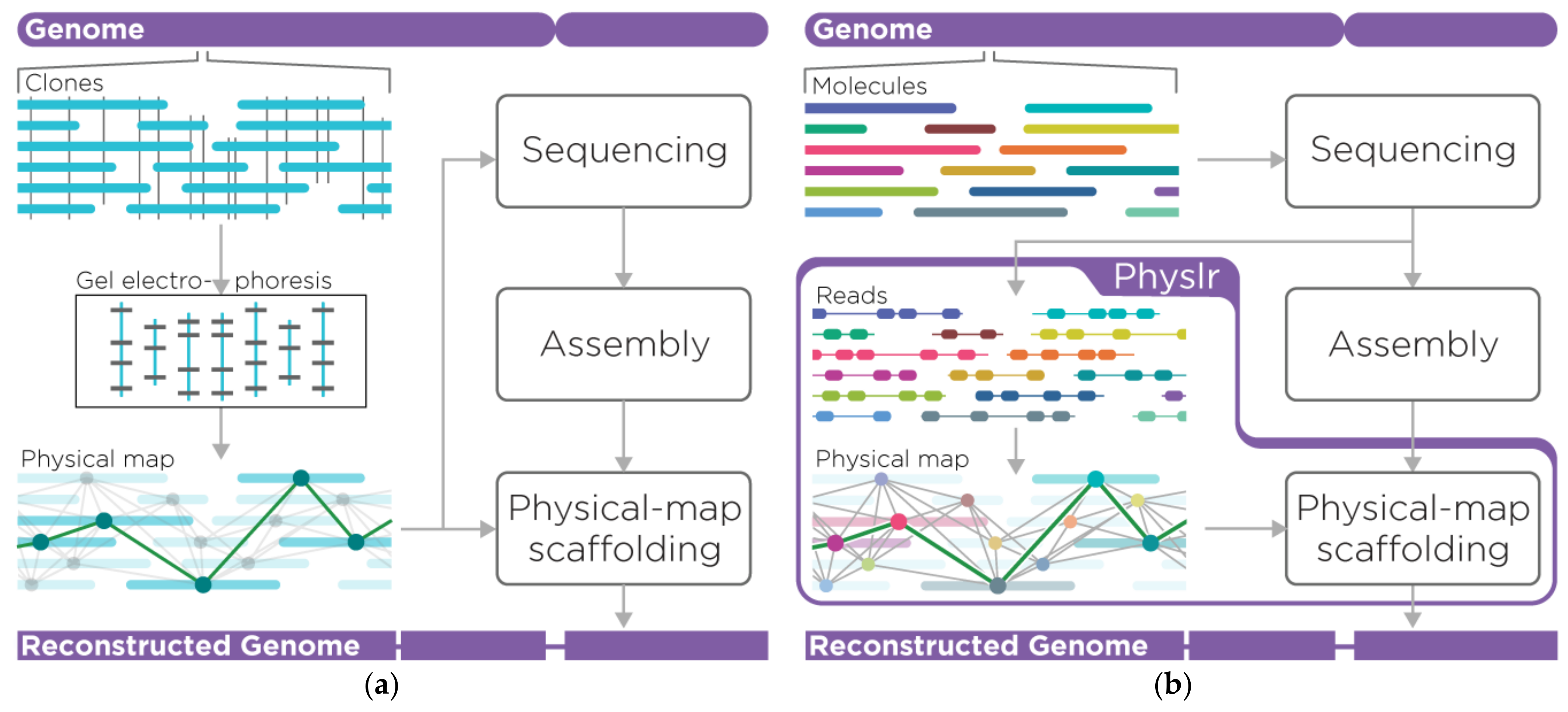
1. Introduction
2. Materials and Methods
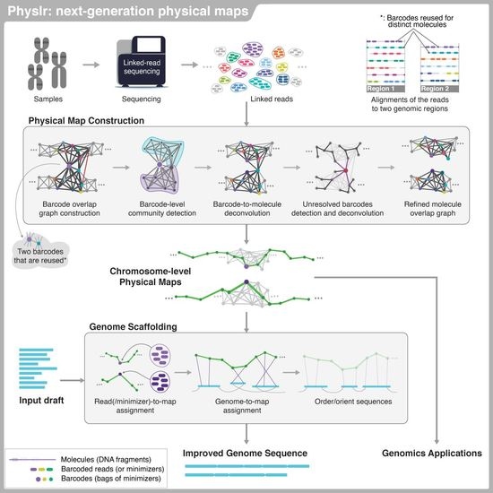
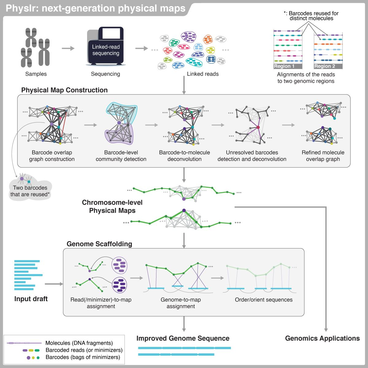
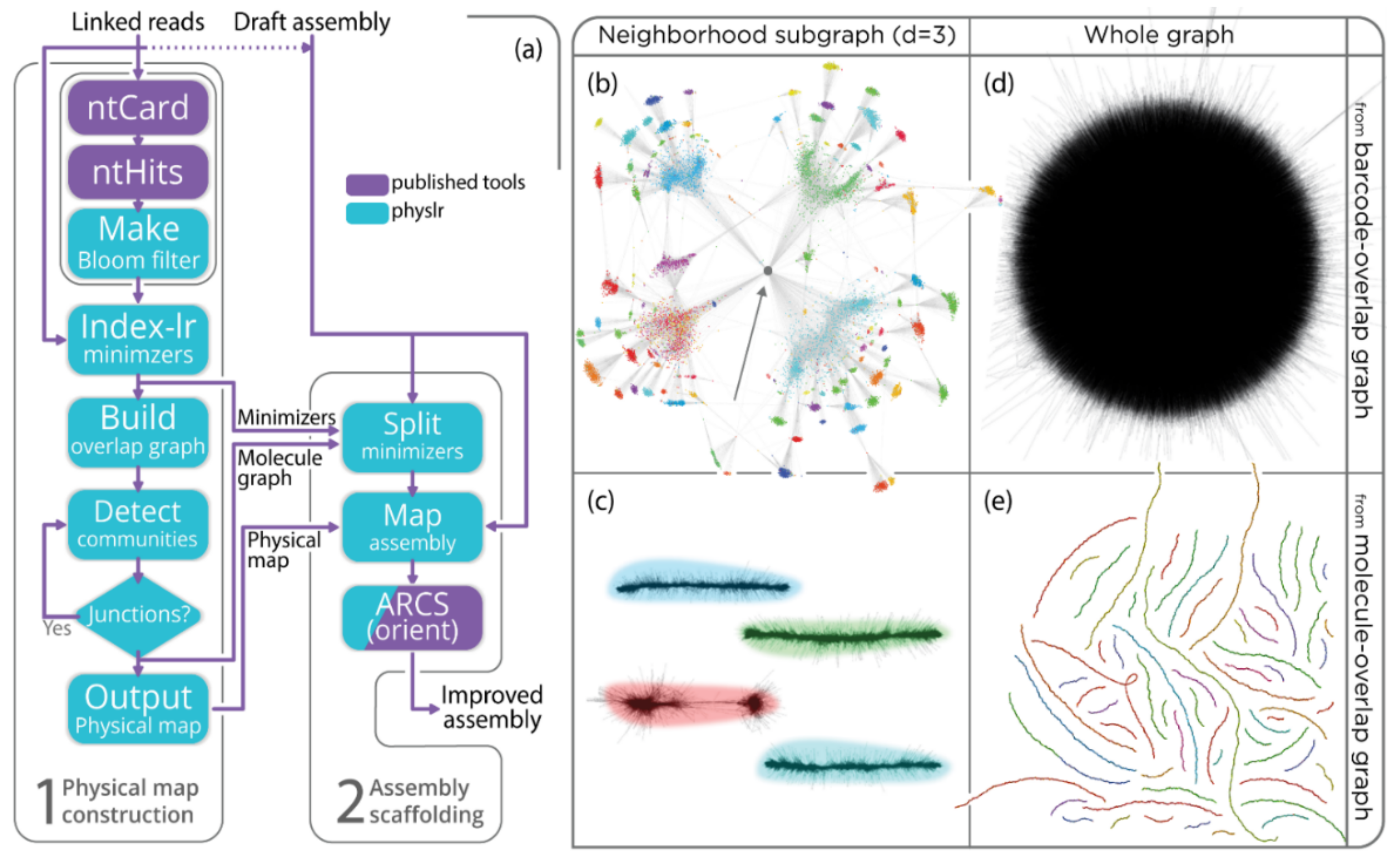
2.1. Overview of the Pipeline
2.2. Physlr Implementation, Stage 1: Constructing Physical Maps
2.3. Physlr Implementation, Stage 2: Scaffolding Draft Assemblies
2.4. Evaluations
3. Results
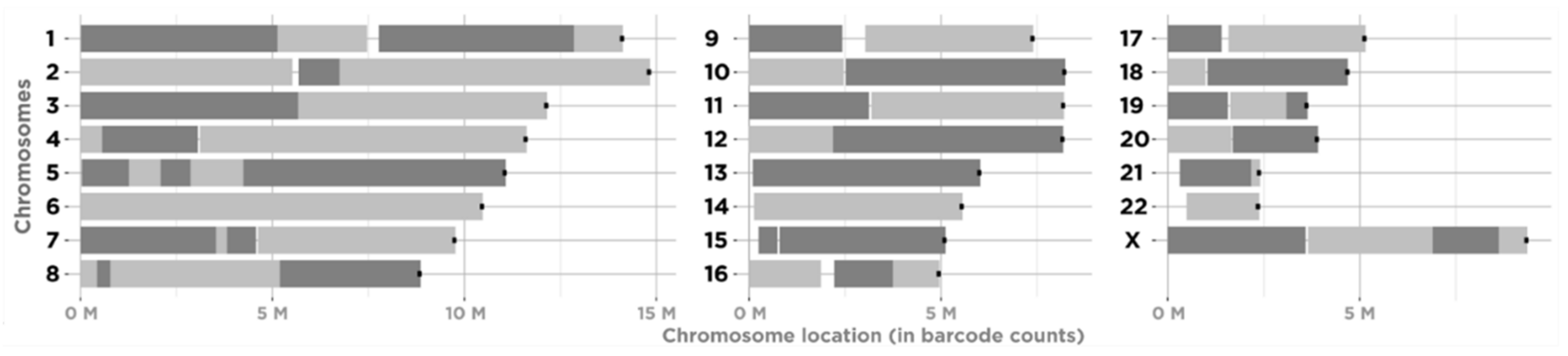
3.1. Constructing Physical Maps
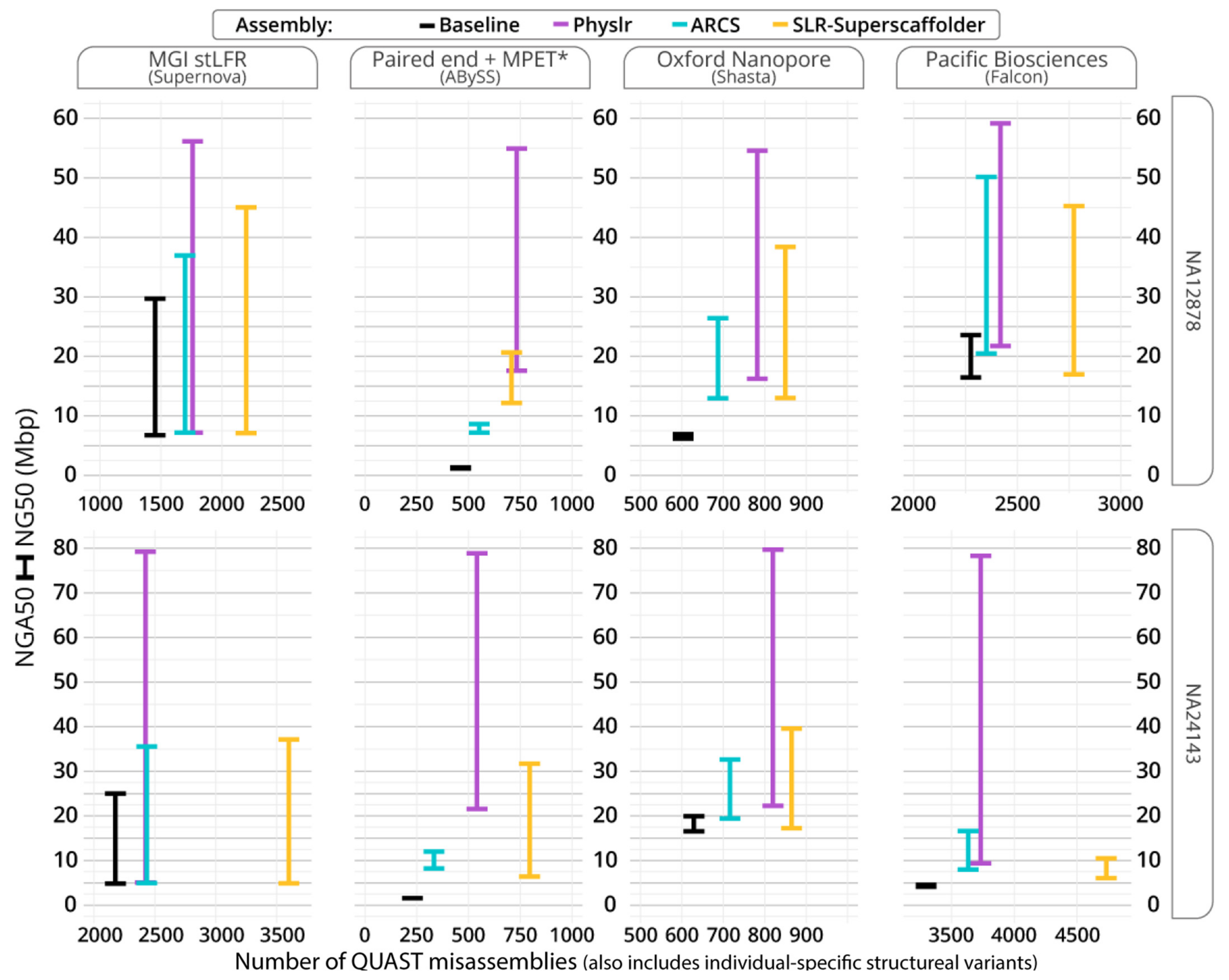
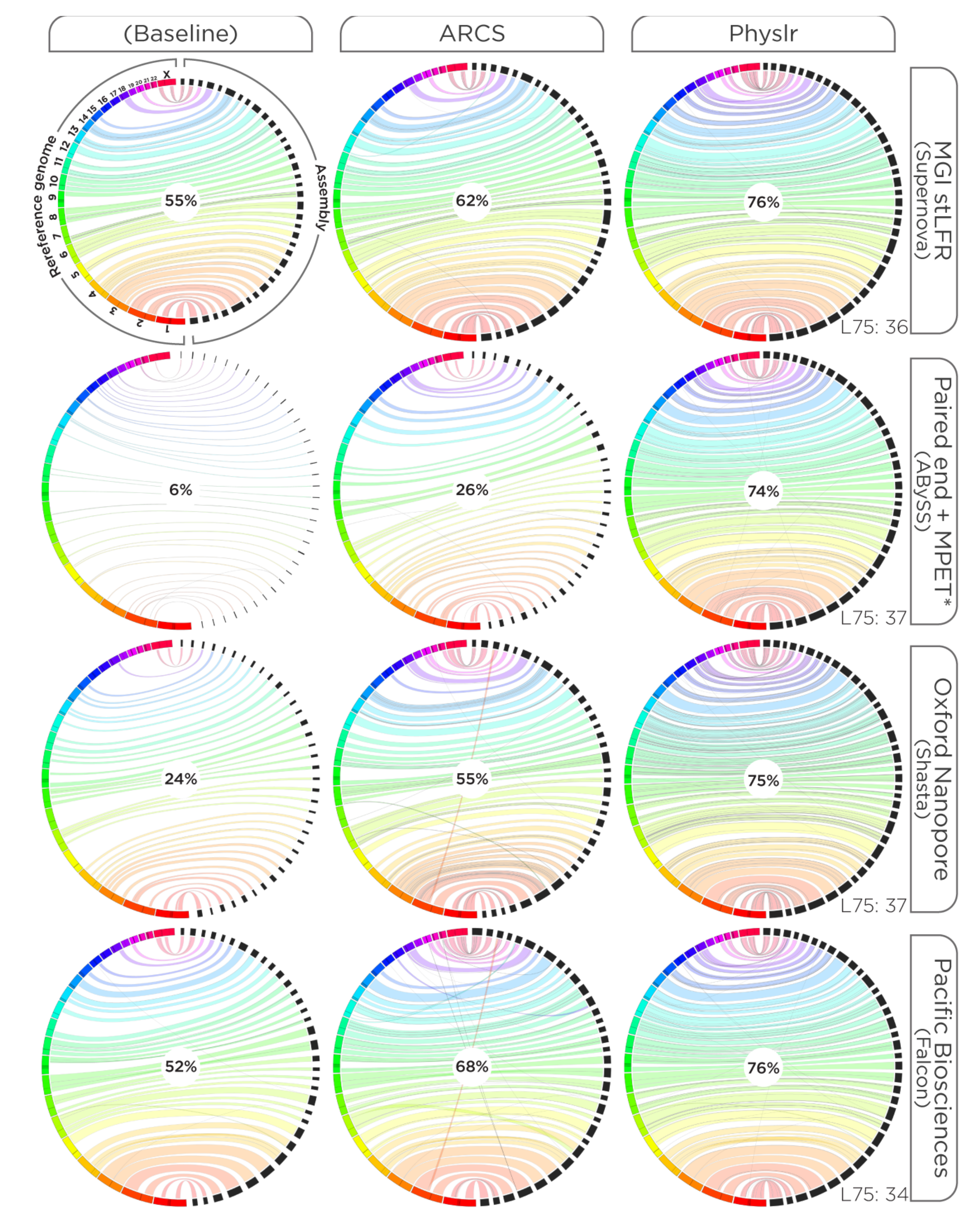
3.2. Scaffolding Draft Assemblies
3.3. Deconvoluting Barcodes via Community Detection
4. Discussion
5. Conclusions
Supplementary Materials
Author Contributions
Funding
Institutional Review Board Statement
Informed Consent Statement
Data Availability Statement
Acknowledgments
Conflicts of Interest
References
- Lewin, H.A.; Larkin, D.M.; Pontius, J.; O’Brien, S.J. Every Genome Sequence Needs a Good Map. Genome Res. 2009, 19, 1925. [Google Scholar] [CrossRef] [PubMed] [Green Version]
- Rice, E.S.; Green, R.E. New Approaches for Genome Assembly and Scaffolding. Annu. Rev. Anim. Biosci. 2019, 7, 17–40. [Google Scholar] [CrossRef] [PubMed]
- Giani, A.M.; Gallo, G.R.; Gianfranceschi, L.; Formenti, G. Long Walk to Genomics: History and Current Approaches to Genome Sequencing and Assembly. Comput. Struct. Biotechnol. J. 2020, 18, 9–19. [Google Scholar] [CrossRef] [PubMed]
- McPherson, J.D.; Marra, M.; Hillier, L.D.; Waterston, R.H.; Chinwalla, A.; Wallis, J.; Sekhon, M.; Wylie, K.; Mardis, E.R.; Wilson, R.K.; et al. A Physical Map of the Human Genome. Nature 2001, 409, 934–941. [Google Scholar] [CrossRef] [Green Version]
- Zhang, H.B.; Wu, C. BAC as Tools for Genome Sequencing. Plant Physiol. Biochem. 2001, 39, 195–209. [Google Scholar] [CrossRef]
- Green, E.D. Strategies for the Systematic Sequencing of Complex Genomes. Nat. Rev. Genet. 2001, 2, 573–583. [Google Scholar] [CrossRef]
- Goffeau, A.; Aert, R.; Agostini-Carbone, M.L.; Ahmed, A.; Aigle, M.; Alberghina, L.; Albermann, K.; Albers, M.; Aldea, M.; Alexandraki, D.; et al. The Yeast Genome Directory. Nature 1997, 387, 5. [Google Scholar] [CrossRef]
- Equence, C.E.S.; Iology, T.O.B.; The, C.; Consortium, S. Genome Sequence of the Nematode C. Elegans: A Platform for Investigating Biology. Science 1998, 282, 2012–2018. [Google Scholar] [CrossRef]
- Mayer, K.; Schüller, C.; Wambutt, R.; Murphy, G.; Volckaert, G.; Pohl, T.; Düsterhöft, A.; Stiekema, W.; Entian, K.D.; Terryn, N.; et al. Sequence and Analysis of Chromosome 4 of the Plant Arabidopsis Thaliana. Nature 1999, 402, 769–777. [Google Scholar] [CrossRef]
- Lander, E.S.; Linton, L.M.; Birren, B.; Nusbaum, C.; Zody, M.C.; Baldwin, J.; Devon, K.; Dewar, K.; Doyle, M.; Fitzhugh, W.; et al. Initial Sequencing and Analysis of the Human Genome. Nature 2001, 409, 860–921. [Google Scholar] [CrossRef] [Green Version]
- Collins, F.S.; McKusick, V.A. Implications of the Human Genome Project for Medical Science. J. Am. Med. Assoc. 2001, 285, 540–544. [Google Scholar] [CrossRef] [PubMed] [Green Version]
- Skolnick, J.; Fetrow, J.S. From Genes to Protein Structure and Function: Novel Applications of Computational Approaches in the Genomic Era. Trends Biotechnol. 2000, 18, 34–39. [Google Scholar] [CrossRef]
- Human Genome Project FAQ. Available online: https://www.genome.gov/human-genome-project/Completion-FAQ (accessed on 16 October 2021).
- Craig Venter, J.; Adams, M.D.; Myers, E.W.; Li, P.W.; Mural, R.J.; Sutton, G.G.; Smith, H.O.; Yandell, M.; Evans, C.A.; Holt, R.A.; et al. The Sequence of the Human Genome. Science 2001, 291, 1304–1351. [Google Scholar] [CrossRef] [Green Version]
- Weber, J.L.; Myers, E.W. Human Whole-Genome Shotgun Sequencing. Genome Res. 1997, 7, 401–409. [Google Scholar] [CrossRef] [PubMed] [Green Version]
- Warren, R.L.; Varabei, D.; Platt, D.; Huang, X.; Messina, D.; Yang, S.P.; Kronstad, J.W.; Krzywinski, M.; Warren, W.C.; Wallis, J.W.; et al. Physical Map-Assisted Whole-Genome Shotgun Sequence Assemblies. Genome Res. 2006, 16, 768. [Google Scholar] [CrossRef] [PubMed] [Green Version]
- Schloss, J.A. How to Get Genomes at One Ten-Thousandth the Cost. Nat. Biotechnol. 2008, 26, 1113–1115. [Google Scholar] [CrossRef]
- Reuter, J.A.; Spacek, D.V.; Snyder, M.P. Review High-Throughput Sequencing Technologies. Mol. Cell 2015, 58, 586–597. [Google Scholar] [CrossRef] [Green Version]
- Das, S.K.; Austin, M.D.; Akana, M.C.; Deshpande, P.; Cao, H.; Xiao, M. Single Molecule Linear Analysis of DNA in Nano-Channel Labeled with Sequence Specific Fluorescent Probes. Nucleic Acids Res. 2010, 38, e177. [Google Scholar] [CrossRef]
- Lam, E.T.; Hastie, A.; Lin, C.; Ehrlich, D.; Das, S.K.; Austin, M.D.; Deshpande, P.; Cao, H.; Nagarajan, N.; Xiao, M.; et al. Genome Mapping on Nanochannel Arrays for Structural Variation Analysis and Sequence Assembly. Nat. Biotechnol. 2012, 30, 771–776. [Google Scholar] [CrossRef]
- Williams, L.J.S.; Tabbaa, D.G.; Li, N.; Berlin, A.M.; Shea, T.P.; MacCallum, I.; Lawrence, M.S.; Drier, Y.; Getz, G.; Young, S.K.; et al. Paired-End Sequencing of Fosmid Libraries by Illumina. Genome Res. 2012, 22, 2241. [Google Scholar] [CrossRef] [Green Version]
- Li, R.; Hsieh, C.L.; Young, A.; Zhang, Z.; Ren, X.; Zhao, Z. Illumina Synthetic Long Read Sequencing Allows Recovery of Missing Sequences Even in the “Finished” C. Elegans Genome. Sci. Rep. 2015, 5, 10814. [Google Scholar] [CrossRef] [PubMed] [Green Version]
- Zheng, G.X.Y.; Lau, B.T.; Schnall-Levin, M.; Jarosz, M.; Bell, J.M.; Hindson, C.M.; Kyriazopoulou-Panagiotopoulou, S.; Masquelier, D.A.; Merrill, L.; Terry, J.M.; et al. Haplotyping Germline and Cancer Genomes with High-Throughput Linked-Read Sequencing. Nat. Biotechnol. 2016, 34, 303–311. [Google Scholar] [CrossRef]
- Pollard, M.O.; Gurdasani, D.; Mentzer, A.J.; Porter, T.; Sandhu, M.S. Long Reads: Their Purpose and Place. Hum. Mol. Genet. 2018, 27, R234–R241. [Google Scholar] [CrossRef] [PubMed]
- Kai, W.; Kikuchi, K.; Tohari, S.; Chew, A.K.; Tay, A.; Fujiwara, A.; Hosoya, S.; Suetake, H.; Naruse, K.; Brenner, S.; et al. Integration of the Genetic Map and Genome Assembly of Fugu Facilitates Insights into Distinct Features of Genome Evolution in Teleosts and Mammals. Genome Biol. Evol. 2011, 3, 424–442. [Google Scholar] [CrossRef] [PubMed] [Green Version]
- Di Genova, A.; Buena-Atienza, E.; Ossowski, S.; Sagot, M.-F. Efficient Hybrid de Novo Assembly of Human Genomes with WENGAN. Nat. Biotechnol. 2020, 39, 422–430. [Google Scholar] [CrossRef]
- Nurk, S.; Koren, S.; Rhie, A.; Rautiainen, M.; Bzikadze, A.V.; Mikheenko, A.; Vollger, M.R.; Altemose, N.; Uralsky, L.; Gershman, A.; et al. The Complete Sequence of a Human Genome. Science 2022, 376, 44–53. [Google Scholar] [CrossRef]
- Wang, O.; Chin, R.; Cheng, X.; Yan Wu, M.K.; Mao, Q.; Tang, J.; Sun, Y.; Anderson, E.; Lam, H.K.; Chen, D.; et al. Efficient and Unique Cobarcoding of Second-Generation Sequencing Reads from Long DNA Molecules Enabling Cost-Effective and Accurate Sequencing, Haplotyping, and de Novo Assembly. Genome Res. 2019, 29, 798–808. [Google Scholar] [CrossRef] [Green Version]
- Chen, Z.; Pham, L.; Wu, T.C.; Mo, G.; Xia, Y.; Chan, P.L.; Porter, D.; Phan, T.; Che, H.; Tran, H.; et al. Ultralow-Input Single-Tube Linked-Read Library Method Enables Short-Read Second-Generation Sequencing Systems to Routinely Generate Highly Accurate and Economical Long-Range Sequencing Information. Genome Res. 2020, 30, 898–909. [Google Scholar] [CrossRef]
- Mohamadi, H.; Khan, H.; Birol, I. NtCard: A Streaming Algorithm for Cardinality Estimation in Genomics Data. Bioinformatics 2017, 33, 1324–1330. [Google Scholar] [CrossRef] [Green Version]
- Mohamadi, H.; Chu, J.; Coombe, L.; Warren, R.; Birol, I. NtHits: De Novo Repeat Identification of Genomics Data Using a Streaming Approach. bioRxiv 2020. [Google Scholar] [CrossRef]
- Roberts, M.; Hayes, W.; Hunt, B.R.; Mount, S.M.; Yorke, J.A. Reducing Storage Requirements for Biological Sequence Comparison. Bioinformatics 2004, 20, 3363–3369. [Google Scholar] [CrossRef] [PubMed] [Green Version]
- Pearl, J. Reverend Bayes on Inference Engines: A Distributed Hierarchical Approach. In Proceedings of the Second AAAI Conference on Artificial Intelligence, Pittsburgh, PA, USA, 18 August 1982; pp. 133–136. [Google Scholar]
- Coombe, L.; Zhang, J.; Vandervalk, B.P.; Chu, J.; Jackman, S.D.; Birol, I.; Warren, R.L. ARKS: Chromosome-Scale Scaffolding of Human Genome Drafts with Linked Read Kmers. BMC Bioinform. 2018, 19, 234. [Google Scholar] [CrossRef] [PubMed] [Green Version]
- Yeo, S.; Coombe, L.; Warren, R.L.; Chu, J.; Birol, I. ARCS: Scaffolding Genome Drafts with Linked Reads. Bioinformatics 2018, 34, 725–731. [Google Scholar] [CrossRef] [PubMed]
- Guo, L.; Xu, M.; Wang, W.; Gu, S.; Zhao, X.; Chen, F.; Wang, O.; Xu, X.; Seim, I.; Fan, G.; et al. SLR-Superscaffolder: A de Novo Scaffolding Tool for Synthetic Long Reads Using a Top-to-Bottom Scheme. BMC Bioinform. 2021, 22, 158. [Google Scholar] [CrossRef] [PubMed]
- Weisenfeld, N.I.; Kumar, V.; Shah, P.; Church, D.M.; Jaffe, D.B. Direct Determination of Diploid Genome Sequences. Genome Res. 2017, 27, 757–767. [Google Scholar] [CrossRef] [Green Version]
- Jackman, S.D.; Vandervalk, B.P.; Mohamadi, H.; Chu, J.; Yeo, S.; Hammond, S.A.; Jahesh, G.; Khan, H.; Coombe, L.; Warren, R.L.; et al. ABySS 2.0: Resource-Efficient Assembly of Large Genomes Using a Bloom Filter Effect of Bloom Filter False Positive Rate. Genome Res. 2017, 27, 768–777. [Google Scholar] [CrossRef] [Green Version]
- Shafin, K.; Pesout, T.; Lorig-Roach, R.; Haukness, M.; Olsen, H.E.; Bosworth, C.; Armstrong, J.; Tigyi, K.; Maurer, N.; Koren, S.; et al. Nanopore Sequencing and the Shasta Toolkit Enable Efficient de Novo Assembly of Eleven Human Genomes. Nat. Biotechnol. 2020, 38, 1044–1053. [Google Scholar] [CrossRef]
- Chin, C.-S.; Peluso, P.; Sedlazeck, F.J.; Nattestad, M.; Concepcion, G.T.; Clum, A.; Dunn, C.; O’Malley, R.; Figueroa-Balderas, R.; Morales-Cruz, A.; et al. Phased Diploid Genome Assembly with Single-Molecule Real-Time Sequencing. Nat. Methods 2016, 13, 1050–1054. [Google Scholar] [CrossRef] [Green Version]
- Gurevich, A.; Saveliev, V.; Vyahhi, N.; Tesler, G. QUAST: Quality Assessment Tool for Genome Assemblies. Bioinformatics 2013, 29, 1072–1075. [Google Scholar] [CrossRef]
- Chu, J. Jupiter Plot: A Circos-Based Tool to Visualize Genome Assembly Consistency (Version 1.0). Zenodo. 2018. Available online: https://zenodo.org/record/1241235#.YqEDN6hlBD9 (accessed on 6 June 2022).
- Krzywinski, M.; Schein, J.; Birol, I.; Connors, J.; Gascoyne, R.; Horsman, D.; Jones, S.J.; Marra, M.A. Circos: An Information Aesthetic for Comparative Genomics. Genome Res. 2009, 19, 1639–1645. [Google Scholar] [CrossRef] [Green Version]
- Danko, D.C.; Meleshko, D.; Bezdan, D.; Mason, C.; Hajirasouliha, I. Minerva: An Alignment- and Reference-Free Approach to Deconvolve Linked-Reads for Metagenomics. Genome Res. 2019, 29, 116–124. [Google Scholar] [CrossRef] [PubMed] [Green Version]
- Palla, G.; Derényi, I.; Farkas, I.; Vicsek, T. Uncovering the Overlapping Community Structure of Complex Networks in Nature and Society. Nature 2005, 435, 814–818. [Google Scholar] [CrossRef] [PubMed] [Green Version]
- Blondel, V.D.; Guillaume, J.L.; Lambiotte, R.; Lefebvre, E. Fast Unfolding of Communities in Large Networks. J. Stat. Mech. Theory Exp. 2008, 2008, P10008. [Google Scholar] [CrossRef] [Green Version]
- Newman, M.E.J.; Girvan, M. Finding and Evaluating Community Structure in Networks. Phys. Rev. E 2004, 69, 026113. [Google Scholar] [CrossRef] [PubMed] [Green Version]
- Mori, B.A.; Coutu, C.; Chen, Y.H.; Campbell, E.O.; Dupuis, J.R.; Erlandson, M.A.; Hegedus, D.D. De Novo Whole Genome Assembly of the Swede Midge (Contarinia nasturtii), a Specialist of Brassicaceae, Using Linked-Read Sequencing. Genome Biol. Evol. 2021, 13, evab036. [Google Scholar] [CrossRef]
- Engler, J.O.; Lawrie, Y.; Gansemans, Y.; van Nieuwerburgh, F.; Suh, A.; Lens, L. Genome Report: De Novo Genome Assembly and Annotation for the Taita White-Eye (Zosterops Silvanus). bioRxiv 2020. [Google Scholar] [CrossRef] [Green Version]
- Brian Simison, W.; Parham, J.F.; Papenfuss, T.J.; Lam, A.W.; Henderson, J.B. An Annotated Chromosome-Level Reference Genome of the Red-Eared Slider Turtle (Trachemys Scripta Elegans). Genome Biol. Evol. 2020, 12, 456–462. [Google Scholar] [CrossRef]
- Roodgar, M.; Babveyh, A.; Nguyen, L.H.; Zhou, W.; Sinha, R.; Lee, H.; Hanks, J.B.; Avula, M.; Jiang, L.; Jian, R.; et al. Chromosome-Level de Novo Assembly of the Pig-Tailed Macaque Genome Using Linked-Read Sequencing and HiC Proximity Scaffolding. Gigascience 2020, 9, giaa069. [Google Scholar] [CrossRef]
- Helmkampf, M.; Bellinger, M.R.; Geib, S.M.; Sim, S.B.; Takabayashi, M. Draft Genome of the Rice Coral Montipora Capitata Obtained from Linked-Read Sequencing. Genome Biol. Evol. 2019, 11, 2045–2054. [Google Scholar] [CrossRef] [Green Version]
- Zhou, X.; Zhang, L.; Weng, Z.; Dill, D.L.; Sidow, A. Aquila Enables Reference-Assisted Diploid Personal Genome Assembly and Comprehensive Variant Detection Based on Linked Reads. Nat. Commun. 2021, 12, 1077. [Google Scholar] [CrossRef]
- Onore, M.E.; Torella, A.; Musacchia, F.; D’Ambrosio, P.; Zanobio, M.; del Vecchio Blanco, F.; Piluso, G.; Nigro, V. Linked-Read Whole Genome Sequencing Solves a Double DMD Gene Rearrangement. Genes 2021, 12, 133. [Google Scholar] [CrossRef] [PubMed]
- Fang, L.; Kao, C.; Gonzalez, M.V.; Mafra, F.A.; Pellegrino da Silva, R.; Li, M.; Wenzel, S.S.; Wimmer, K.; Hakonarson, H.; Wang, K. LinkedSV for Detection of Mosaic Structural Variants from Linked-Read Exome and Genome Sequencing Data. Nat. Commun. 2019, 10, 5585. [Google Scholar] [CrossRef] [PubMed] [Green Version]
- Teague, B.; Waterman, M.S.; Goldstein, S.; Potamousis, K.; Zhou, S.; Reslewic, S.; Sarkar, D.; Valouev, A.; Churas, C.; Kidd, J.M.; et al. High-Resolution Human Genome Structure by Single-Molecule Analysis. Proc. Natl. Acad. Sci. USA 2010, 107, 10848–10853. [Google Scholar] [CrossRef] [PubMed] [Green Version]
- Dréau, A.; Venu, V.; Avdievich, E.; Gaspar, L.; Jones, F.C. Genome-Wide Recombination Map Construction from Single Individuals Using Linked-Read Sequencing. Nat. Commun. 2019, 10, 4309. [Google Scholar] [CrossRef] [Green Version]
- Xu, M.; Guo, L.; Du, X.; Li, L.; Peters, B.A.; Deng, L.; Wang, O.; Chen, F.; Wang, J.; Jiang, Z.; et al. Accurate Haplotype-Resolved Assembly Reveals the Origin of Structural Variants for Human Trios. Bioinformatics 2021, 37, 2095–2102. [Google Scholar] [CrossRef]
- Chaisson, M.J.P.; Sanders, A.D.; Zhao, X.; Malhotra, A.; Porubsky, D.; Rausch, T.; Gardner, E.J.; Rodriguez, O.L.; Guo, L.; Collins, R.L.; et al. Multi-Platform Discovery of Haplotype-Resolved Structural Variation in Human Genomes. Nat. Commun. 2019, 10, 1784. [Google Scholar] [CrossRef] [Green Version]
- Udall, J.A.; Dawe, R.K. Is It Ordered Correctly? Validating Genome Assemblies by Optical Mapping. Plant Cell 2018, 30, 7–14. [Google Scholar] [CrossRef] [Green Version]
- Jackman, S.D.; Coombe, L.; Chu, J.; Warren, R.L.; Vandervalk, B.P.; Yeo, S.; Xue, Z.; Mohamadi, H.; Bohlmann, J.; Jones, S.J.M.; et al. Tigmint: Correcting Assembly Errors Using Linked Reads from Large Molecules. BMC Bioinform. 2018, 19, 393. [Google Scholar] [CrossRef] [Green Version]
- Rhie, A.; McCarthy, S.A.; Fedrigo, O.; Damas, J.; Formenti, G.; Koren, S.; Uliano-Silva, M.; Chow, W.; Fungtammasan, A.; Kim, J.; et al. Towards Complete and Error-Free Genome Assemblies of All Vertebrate Species. Nature 2021, 592, 737–746. [Google Scholar] [CrossRef]
- Cheng, H.; Concepcion, G.T.; Feng, X.; Zhang, H.; Li, H. Haplotype-Resolved de Novo Assembly Using Phased Assembly Graphs with Hifiasm. Nat. Methods 2021, 18, 170–175. [Google Scholar] [CrossRef]
- Nurk, S.; Walenz, B.P.; Rhie, A.; Vollger, M.R.; Logsdon, G.A.; Grothe, R.; Miga, K.H.; Eichler, E.E.; Phillippy, A.M.; Koren, S. HiCanu: Accurate Assembly of Segmental Duplications, Satellites, and Allelic Variants from High-Fidelity Long Reads. Genome Res. 2020, 30, 1291–1305. [Google Scholar] [CrossRef] [PubMed]
- Javed, M.A.; Younis, M.S.; Latif, S.; Qadir, J.; Baig, A. Community Detection in Networks: A Multidisciplinary Review. J. Netw. Comput. Appl. 2018, 108, 87–111. [Google Scholar] [CrossRef]

Publisher’s Note: MDPI stays neutral with regard to jurisdictional claims in published maps and institutional affiliations. |
© 2022 by the authors. Licensee MDPI, Basel, Switzerland. This article is an open access article distributed under the terms and conditions of the Creative Commons Attribution (CC BY) license (https://creativecommons.org/licenses/by/4.0/).
Share and Cite
Afshinfard, A.; Jackman, S.D.; Wong, J.; Coombe, L.; Chu, J.; Nikolic, V.; Dilek, G.; Malkoç, Y.; Warren, R.L.; Birol, I. Physlr: Next-Generation Physical Maps. DNA 2022, 2, 116-130. https://doi.org/10.3390/dna2020009
Afshinfard A, Jackman SD, Wong J, Coombe L, Chu J, Nikolic V, Dilek G, Malkoç Y, Warren RL, Birol I. Physlr: Next-Generation Physical Maps. DNA. 2022; 2(2):116-130. https://doi.org/10.3390/dna2020009
Chicago/Turabian StyleAfshinfard, Amirhossein, Shaun D. Jackman, Johnathan Wong, Lauren Coombe, Justin Chu, Vladimir Nikolic, Gokce Dilek, Yaman Malkoç, René L. Warren, and Inanc Birol. 2022. "Physlr: Next-Generation Physical Maps" DNA 2, no. 2: 116-130. https://doi.org/10.3390/dna2020009
APA StyleAfshinfard, A., Jackman, S. D., Wong, J., Coombe, L., Chu, J., Nikolic, V., Dilek, G., Malkoç, Y., Warren, R. L., & Birol, I. (2022). Physlr: Next-Generation Physical Maps. DNA, 2(2), 116-130. https://doi.org/10.3390/dna2020009