


Abstract
We examine the growth of Internet Protocol version 6 (IPv6) routing state from 2010 to 2025. The global IPv4 address space has been exhausted, and the transition to IPv6 is ongoing. Using publicly accessible data from the RIPE Route Collectors (RRCs), we show that growth in the number of globally visible IPv6 routing prefixes follows different models over time, reflecting different growth patterns: exponential, power-law, and stretched-exponential. In addition to building models using publicly available RIPE data, we use this data source to demonstrate that our analysis holds across different Internet Exchange Points (IXPs) around the world and has predictive value. We provide in-depth analyses of IPv6 routing state growth, and we believe these are the first such analyses. Additionally, we highlight previous similar analyses of other aspects of network characteristics (such as topology and network traffic), and show that our analyses provide new insights. Specifically, we show the following: (1) previous models that have worked well for other network characteristics do not work well for routing state; (2) growth patterns for IPv6 routing state have changed significantly over time; (3) growth patterns cannot be described by a single model, and need to be analysed in a piecewise fashion; (4) fitting of previous data might not necessarily result in good predictive quality, and we identify the factors that may affect the predictive quality of a model and the predictive models that are suitable at the current time. Our analyses include metrics for assessing model fit. Overall, we observe a decrease in the rate of growth of IPv6 routing state, while the overall use of IPv6 continues to grow. We provide a critical evaluation of our approach, and also discuss possible factors affecting the growth of global IPv6 routing state.
1. Introduction
The global Internet routing system maintains a distributed representation of reachable address space through routers sharing state via the Border Gateway Protocol (BGP). The size and growth of this routing state, typically measured by the number of distinct routing prefixes (also called address prefixes or simply prefixes) visible in routing tables, has long been recognised as a key factor in assessing the scalability of the global routing system for IPv6 (as well as for IPv4). Growth in routing state has a direct impact on network routers: memory requirements, forwarding performance, control-plane dynamics, and the convergence time for consistency after a change in routing state. Concern over such issues and the potential impact on the operational stability of the Internet have motivated architectural proposals for better managing this state.
Historically, the evolution of Internet routing has been studied through the lens of topology, traffic volumes and patterns, and protocol behaviour. While these perspectives provide important insights, they do not directly address the statistical structure of routing state growth itself. In particular, it remains unclear whether routing state evolves according to unbounded growth processes, such as exponential or power-law models, or whether it exhibits transitions toward constrained, saturating regimes. Such information would be valuable to network operators, as well as to designers of network hardware.
This question has become increasingly relevant in the context of IPv6. Unlike IPv4, which is subject to address exhaustion, IPv6 provides a vastly larger address space, potentially enabling continued expansion of routing state. At the same time, operational practices such as multi-homing, traffic engineering, and policy-driven announcements introduce competing pressures that impact the growth of routing state.
Understanding the statistical form of routing state evolution is therefore important for both theoretical and practical reasons. From a modelling perspective, it informs the choice of appropriate growth laws and the interpretation of observed heavy-tailed behaviour. From an operational perspective, it informs capacity planning, including router provisioning and control-plane design, and provides insight into the long-term scalability of the routing system.
1.1. Problem Statement
The problem addressed in this study is twofold. First, we seek to determine how existing IPv6 routing state can be modelled from historical observations: whether its growth is better described by unbounded models such as exponential or power-law forms, by intermediate heavy-tailed models, or by constrained sigmoidal forms. This distinction matters because apparent power-law behaviour in empirical Internet data can be misleading without careful model comparison and validation [1,2]. Secondly, we seek to determine how such models can be used to predict future IPv6 routing state in a way that is useful to those who run, operate, provision, and plan networks. By combining historical measurement with predictive modelling, this study aims to provide evidence about where IPv6 routing state has been and where it is likely to be heading, so that operational planning can be grounded in measured routing dynamics rather than extrapolation alone.
Growth in the global Internet routing state is a continuing operational concern because the routing system must store, process, and disseminate reachability information on a global scale. As the number of visible prefixes and routing updates increases, routers must maintain larger routing and forwarding state, while BGP control-plane mechanisms must process more announcements and withdrawals and still converge after policy or reachability changes. Prior work has shown that Internet routing convergence can be delayed after routing changes [3], and earlier analyses of BGP routing-table growth documented the operational significance of sustained increases in advertised prefixes [4,5]. Although aggregation mechanisms such as CIDR were introduced to reduce pressure on routing-table growth [6], operational practices including multi-homing, traffic engineering, policy-driven deaggregation, and IPv6 address-assignment choices continue to shape the amount of routing state visible in the global routing system [7,8].
A second aspect of the problem is provisioning. Network equipment is designed with finite memory and processing capacity, so operators must decide whether deployed and planned routers can hold the required routing and forwarding state, absorb control-plane updates, and converge without threatening operational stability. This planning problem is especially important for IPv6: the much larger IPv6 address space removes the address-exhaustion constraint that shaped IPv4, but it does not remove the operational and architectural constraints associated with globally visible routing state. Prior measurement studies have described IPv6 deployment, topology, routing, and performance [9,10], while measurement infrastructures such as RIPE RIS and Route Views provide the longitudinal BGP data needed to study routing state over time [11,12]. Recent measurement work reinforces that this is not only a static forwarding-table capacity problem. Traffic-engineering events can contribute materially to BGP updates and convergence time, while long-lived BGP “zombies” show that stale routes may persist after withdrawals [13,14]. Routing-state growth, therefore, has to be understood both as a provisioning problem, concerned with whether deployed equipment can store and process the required state, and as a dynamic control-plane problem, concerned with whether routing updates propagate and converge reliably.
1.2. Contributions
This study investigated the statistical structure of IPv6 routing prefix growth between 2010 and 2025, using data from multiple RIPE Routing Information Service (RIS) route collectors (RIPE RRCs). We then evaluated a range of alternative growth models, including unbounded and saturating forms, and assessed their relative performance using model selection criteria and rolling backtests. This approach enabled direct comparison of predictive accuracy across different time periods—fitting windows—and allowed identification of changes in the underlying growth regime.
By combining longitudinal measurement data with comparative model fitting and out-of-sample evaluation, this study provides new empirical evidence regarding the evolution of IPv6 routing state. In particular, it addresses whether routing growth is best characterised as a single process or as a sequence of piecewise, regime-dependent behaviours, and whether current trends are consistent with continued expansion or the emergence of a constrained steady state.
We constructed a longitudinal time series of IPv6 routing prefix visibility from multiple RIPE RIS collectors over the period 2010 to 2025. We evaluated a range of candidate growth models, including heavy-tailed, exponential, and saturating forms, and assessed their predictive performance using rolling backtests. The results provided evidence for regime-dependent growth behaviour and supported the interpretation that IPv6 routing state is transitioning toward a constrained, sigmoidal regime.
The modelling equations used later in this paper are included to test a deliberately broad set of plausible explanations for IPv6 routing-state growth, rather than to assume a single model in advance. The linear model is retained as a simple reference case: if more complex models do not improve substantially over constant incremental growth, then acceleration or saturation should not be claimed. The power-law model is included because power-law and scale-free explanations have been influential in Internet topology and Internet measurement, but such claims need to be tested rather than assumed [1,2,15]. The exponential model captures unconstrained multiplicative growth expected during an early technology-deployment phase, while the stretched-exponential model allows sub-exponential growth arising from heterogeneous adoption rates and multiple operational timescales [16]. The saturating power-law model provides an intermediate case in which initially scale-law growth is eventually constrained by finite operational resources [17]. Finally, the logistic, Gompertz, and Richards models are included because routing-state growth is also a deployment and diffusion process: IPv6 adoption may initially accelerate but later decelerate as large providers deploy IPv6, aggregation practices stabilise, and the marginal number of additional globally visible prefixes falls [4,5,18]. This candidate set therefore spans constant, heavy-tailed, exponential, heterogeneous, and constrained growth regimes, which is necessary for testing whether IPv6 routing state remains in an expansionary regime or is moving toward saturation. We return to the interpretation and validity of this comparison in Section 5.2.
1.3. Structure of This Paper
The remainder of this paper is structured as follows. Section 2 reviews the relevant literature on Internet growth, routing measurement, and statistical modelling. Section 3 describes the data and modelling framework we have used in our study. Section 4 presents empirical results, followed by a discussion of the implications as well as some suggestions as to the underlying reasons for the changing regimes that are observed in Section 5.
2. Background
From a research perspective, Internet growth has been studied across several distinct but related domains:
- Structural topology of the AS-level graph.
- Statistical properties of degree distributions and scaling laws.
- Dynamics of inter-domain routing and BGP behaviour.
- Growth of routing state and routing table size.
- Constraints on scalability, including convergence and memory requirements.
The Internet has long been recognised not merely as a communication infrastructure but as a complex evolving system whose growth reflects architectural principles, operational practice, and economic incentives [19]. Its growth has been studied from multiple disciplinary perspectives, including networking, economics, statistical physics, and complex systems theory.
Early efforts to characterise the Internet’s structure focused on macroscopic topology. It was observed from analysis of topology data that the Autonomous System (AS) level graph exhibits power-law relationships in node degree, path length, and connectivity metrics [15]. This observation was influential, suggesting that Internet growth reflects scale-free dynamics rather than random graph behaviour. Further analyses provided theoretical grounding through preferential attachment models, arguing that network expansion naturally produces heavy-tailed degree distributions [20].
2.1. Measurement Infrastructure and Routing Observability
Rigorous analysis of routing state depends on reliable observation infrastructure. The establishment of the RouteViews project and the RIPE Routing Information Service (RIS) provided continuous archival access to BGP table snapshots from multiple vantage points [11,12]. These systems enabled longitudinal studies of prefix growth, routing churn, and control-plane dynamics.
Subsequent measurement initiatives, such as CAIDA’s Ark infrastructure, expanded the ability to observe topology and reachability from distributed probing platforms [21]. Studies presented at PAM and IMC examined routing convergence, update frequency, AS relationship inference, and the evolution of peering structures [22,23].
Recent work has revisited the route-collector infrastructure on which such longitudinal analyses rely. It was argued that current BGP data-collection platforms face sustainability challenges arising from continued growth, redundancy in collected updates, and incomplete visibility; a next-generation architecture for BGP data collection was proposed [24]. For the present study, this reinforces the need to interpret RIPE RIS observations as collector-specific views of routing state rather than as a single complete view of the global routing system.
The methodological maturation of Internet measurement established several important principles. First, routing visibility is vantage-point dependent. Secondly, prefix advertisements reflect policy choices as well as allocation. Thirdly, routing state growth must be analysed in the context of operational practices for connectivity options, such as multi-homing and traffic engineering.
Despite these advances, most studies have treated routing table size descriptively rather than modelling its distributional form across ranks or over extended time windows.
2.2. Statistical Models of Network Growth
The observation of heavy-tailed distributions in Internet structure prompted extensive debate regarding appropriate statistical methodology. Early work highlighted the importance of critically examining claims of scale-free behaviour in networked systems [1]. However, it was later demonstrated that apparent power-law behaviour must be validated using rigorous maximum likelihood estimation and goodness-of-fit testing [2]. Many empirical datasets previously assumed to follow power laws were shown to exhibit alternative heavy-tailed forms.
In networking research, Zipfian and related distributions have been observed in web object popularity, peer-to-peer traffic, and AS connectivity [25]. The Zipf–Mandelbrot distribution generalises classical Zipf behaviour by incorporating a shift parameter, allowing improved modelling of empirical data exhibiting curvature at lower ranks.
In addition to power-law models, exponential and stretched-exponential forms have been widely used to describe growth processes in complex systems [16]. Exponential growth frequently arises in early phases of technological diffusion, while stretched-exponential behaviour reflects heterogeneous processes operating across multiple scales [18].
These observations suggest that growth in networked systems may not be well described by a single global distribution. Instead, different phases of system evolution may exhibit distinct statistical behaviour, reflecting changing technological and operational conditions.
2.3. IPv4 Routing Growth and Architectural Limits
During the expansionary phase of IPv4, the routing table size increased steadily despite the use of Classless Inter-Domain Routing (CIDR) to mitigate aggregation pressure [6]. Multi-homing, traffic engineering, and policy-driven deaggregation contributed to sustained growth in globally visible prefixes.
Before the year 2000, before more mainstream IPv6 adoption, longitudinal analyses documented the increase in advertised IPv4 prefixes and highlighted concerns regarding routing scalability [4,5]. Academic studies similarly examined BGP update rates and routing stability under increasing table sizes for IPv4 [3]. However, IPv4 growth was bounded by the finite size of the address space. The exhaustion of the Internet Assigned Numbers Authority (IANA) “free pool” of IPv4 addresses in 2011 marked a structural inflection point. Subsequent growth dynamics reflected transfers of addresses between providers and users, and the fragmentation of the aggregation benefits offered by CIDR, rather than expansion of the underlying resource [9].
This episode illustrated a key theoretical insight: scale-free behaviour observed during expansion may not persist under resource constraints. The literature has not systematically analysed the distributional consequences of exhaustion, but it establishes that growth regimes are sensitive to structural limits [26,27].
2.4. IPv6 Deployment and Control-Plane Evolution
IPv6 was designed with (what was thought to be) an effectively inexhaustible address space, values. Early IPv6 deployment was slow and uneven, driven largely by research networks and early adopters. Following IPv4 exhaustion and World IPv6 Launch, IPv6 adoption accelerated, but recent measurement work shows that deployment is uneven and partial rather than simply present or absent. There are arguments for a non-binary view of IPv6 adoption, measuring how often users and services actually use IPv6 across client, service, and cloud-provider perspectives [28]. This supports the view that IPv6 routing-state growth reflects heterogeneous deployment and operational practice rather than address-space availability alone.
Empirical studies have measured IPv6 traffic share and adoption rates across regions and networks [9]. A study of IPv6 topology has observed structural differences relative to IPv4, including distinct peering patterns [10], and analyses have shown operational environments shaped by Carrier-Grade Network Address Translation (CG-NAT) and dual-stack transitions [29]. These works establish that IPv6 adoption reflects economic incentives, regulatory pressures, and operational constraints. However, they do not model routing prefix visibility growth as a rank-frequency distribution nor evaluate its temporal stability.
Operator reports provide descriptive statistics on IPv6 routing table size, e.g., [5]. Yet formal parametric modelling remains largely absent from the peer-reviewed literature. Crucially, while IPv6 removes the address scarcity constraint present in IPv4, it does not eliminate constraints on routing state. Indeed, although the current best practice for prefix allocation is a 56-bit prefix for a site network [7], operational use might allow IPv6 prefixes of up to 64 bits, and Provider Independent (PI) allocation does not allow CIDR-like aggregation [8]; therefore, there is the potential for IPv6 routing state to be many millions of times greater than that of IPv4.
However, the nature of policy-based routing with BGP means that prefix visibility remains influenced by policy, aggregation behaviour, and economic incentives. As a result, the evolution of IPv6 routing state cannot be inferred directly from address space availability and must instead be examined empirically.
2.5. Diffusion of Innovation and Regime Transition
Technological infrastructures frequently exhibit growth dynamics that evolve over time as adoption progresses. Diffusion theory suggests that technological deployment of innovations often follows sigmoid trajectories characterised by an initial phase of slow growth, followed by rapid expansion, and eventually a period of saturation [18] (see also Appendix B). Such behaviour arises as adoption spreads through networks of organisations and users, while practical, economic, and architectural constraints eventually limit further expansion.
In practice, however, the intermediate phases of technological diffusion need not appear sigmoid when examined over limited time horizons. Early and mid-stage growth may instead exhibit behaviour that resembles exponential or heavy-tailed processes, reflecting heterogeneous adoption across networks, economic incentives for deployment, and evolving operational practices. As a result, different statistical models may describe different phases of system development.
Within Internet infrastructure, routing state growth is influenced not only by address availability but also by routing policy, multi-homing practices, aggregation behaviour, and the economic incentives of network operators. These factors may produce complex growth dynamics in which multiple statistical regimes appear over time. Consequently, models that assume a single global distribution may obscure important transitions in the evolution of routing state.
Understanding whether IPv6 routing growth exhibits such regime changes is therefore an important question for Internet measurement research.
2.6. Summary of Background
Taken together, previous research establishes several key points regarding Internet growth and routing dynamics.
- Internet topology exhibits heavy-tailed structural properties, often approximated by power-law distributions [15].
- Observational analyses of IPv4 routing growth documented sustained increases in globally visible prefixes during the expansionary phase of the Internet [4,5].
- The exhaustion of the IPv4 address space altered the dynamics of routing growth, introducing structural constraints on further expansion [9].
- Research on IPv6 has primarily focused on deployment metrics, topology evolution, and traffic share rather than on the statistical modelling of routing prefix visibility [9,10,29].
- Although heavy-tailed models such as Zipf or Zipf–Mandelbrot distributions are frequently invoked in Internet measurement, alternative models, including exponential and stretched-exponential forms, may also describe complex growth processes.
Consequently, while the previous research provides substantial insight into Internet topology and deployment dynamics, relatively little work has modelled the statistical structure of routing prefix growth itself for IPv6. The interaction between heavy-tailed behaviour, temporal evolution, and structural constraints has not been systematically analysed, nor has it been evaluated in a predictive framework.
The absence of longitudinal statistical modelling of IPv6 routing prefix visibility represents an important gap in the measurement literature. Existing studies provide detailed observations of deployment trends but do not evaluate competing growth models for the evolution of routing state, nor do they assess the predictive validity of such models across time.
In particular, it remains unclear whether the apparent heavy-tailed behaviour observed in routing datasets reflects a genuine power-law process or whether alternative growth regimes provide a more accurate description. Furthermore, the possibility that different phases of IPv6 deployment may exhibit distinct statistical behaviour has not been systematically examined. This limits the ability to determine whether routing growth is fundamentally unbounded or whether it transitions toward a constrained regime.
These questions are not only of theoretical interest. The growth of routing state directly affects router memory requirements, control-plane complexity, and convergence behaviour and performance during times of routing changes. Without a clear understanding of the underlying growth process, it is difficult to make informed decisions about capacity provisioning or to assess the long-term scalability of the routing system.
To make the relationship to prior work explicit, Table 1 summarises the main strands of literature relevant to this study. The purpose of the comparison is not to provide an exhaustive taxonomy, but to distinguish work that studies Internet topology, BGP observability, IPv4 routing growth, IPv6 deployment, and general growth models from work that directly models IPv6 routing-table size as a longitudinal routing-state process. This distinction is important because several prior studies provide essential measurement infrastructure or deployment context, but do not evaluate competing growth laws for collector-specific IPv6 routing-state time series.
Table 1.
Comparison of the present study with related strands of Internet measurement and growth modelling literature.
3. Methods
Our approach used a fixed annual date to sample routing state for six geographically dispersed RRCs. This same date was sampled each year from 2010 to 2025. Thus, each RRC had 16 data samples, each representing the global view of routing data from that RRC.
This section gives details of those data samples, as well as detailing the data processing pipeline, assumptions made, and metrics used for evaluation.
3.1. Fixed Sample Date
For longitudinal comparison, for practical purposes, we chose to use a single fixed calendar date each year rather than a moving window or a fixed weekday. Fixed-date snapshotting is well established in longitudinal BGP measurement: prior studies have used recurring monthly routing-table snapshots on the first day of the month, while other multi-year analyses have used the 15th of each month as a stable anchor for repeated comparison [9,32,33].
The first day of the month was considered but rejected because the RouteViews and RIPE RIS repositories occasionally miss midnight Routing Information Base (RIB) dumps on the first day of the month [32]. After excluding this known first-day archive-boundary issue, 5 May was selected because it provided complete and consistent coverage across the chosen RRCs. Moreover, each yearly sample spans a full 24 h period rather than a single instant; because RouteViews and RIPE RIS archive RIB dumps at intervals of 2 and 8 h, respectively, a full-day sample covers multiple underlying RIB dumps and is therefore less sensitive to any single collector-timing artefact [32].
A fixed calendar date also avoids locking the study to a single weekday pattern, since the weekday associated with that date rotates across years. Accordingly, 5 May is best understood not as an arbitrary convenience date, but as a reproducible, non-boundary annual anchor for longitudinal Internet measurement.
3.2. Measurement Data
For this study, we analysed IPv6 routing prefix visibility between 2010 (one year before the Internet Society’s “Global IPv6 Day” on 8 June 2011 [34]) and 2025. On 5 May 2010, Google’s global IPv6 statistics estimated IPv6 deployment to be at 0.23% [35].
Routing state observations were obtained from the RIPE RRCs. The RIPE RIS provides publicly accessible archives of BGP routing table snapshots collected from multiple vantage points located at IXPs worldwide. Each route collector maintains BGP sessions with multiple peers and records the set of routing prefixes visible from those peers at regular intervals.
Annual observations were derived from RIS archive data by extracting the number of distinct IPv6 prefixes present in the routing table for each collector. This produced a longitudinal dataset capturing the evolution of globally visible IPv6 routing state.
As routing visibility depends on vantage point and peering relationships, different collectors observe slightly different subsets of the global routing system. Rather than aggregating observations across collectors, we treated each collector independently and analysed the resulting time series separately. This approach allowed comparison of routing growth dynamics across geographically and topologically distinct measurement points.
The data were collected from longitudinal observations of the IPv6 routing system obtained from the RIPE Routing Information Service (RIS). Six route collectors were analysed: RRC03, RRC06, RRC11, RRC12, RRC13 and RRC14. RIPE RIS route collectors (RRCs) are deployed at, or closely associated with, particular Internet Exchange Points (IXPs). For the collectors analysed in this study, the corresponding exchanges are: RRC03 (Amsterdam, AMS-IX; also listed with NL-IX), RRC06 (Tokyo, DIX-IE and JPIX), RRC11 (New York, NYIIX), RRC12 (Frankfurt, DE-CIX), RRC13 (Moscow, MSK-IX), and RRC14 (Palo Alto, PAIX). These collectors provided geographically distributed vantage points and offer a consistent view of global routing dynamics over the period 2010–2025.
3.3. Construction of the Routing State Time Series
Let denote the number of distinct IPv6 prefixes visible at collector c in year t. For each collector, we therefore obtain a discrete time series:
These time series describe the evolution of routing table size as observed from individual IXPs. As routing announcements reflect both address allocation and operator policy decisions, such as traffic engineering and multi-homing, the resulting series captures the combined effects of technological deployment and operational behaviour.
Prior to modelling, the time series were inspected for inconsistencies arising from collector outages or changes in peer composition. Observations corresponding to incomplete routing snapshots were excluded. The resulting dataset consisted of continuous annual observations for each collector.
Table 2 summarises the rolling backtesting framework used to evaluate model performance over time. Each window defines a distinct temporal split between a fitting period, used to estimate model parameters, and a subsequent prediction period, used to assess out-of-sample performance. By progressively extending the fitting window, this design allows us to examine how predictive accuracy evolves as more historical routing state data become available.
Table 2.
Backtesting windows used for model fitting and prediction.
Figure 1 gives a methodological workflow used to construct collector-specific IPv6 routing-state time series and evaluate candidate growth models. Solid arrows indicate the principal flow of data products between stages. The dotted arrow denotes the repeated return to the fitting-window stage when progressively extended training intervals are analysed for backtests and regime detection.
Figure 1.
Methodological workflow.
3.4. Candidate Growth Models
The statistical structure of routing growth is not known a priori, see Section 1.2. Previous Internet measurement studies have observed heavy-tailed behaviour in a wide range of network phenomena, including AS connectivity, traffic flows, and content popularity [15,25]. However, subsequent work has emphasised that apparent power-law behaviour can often be explained by alternative heavy-tailed models such as stretched-exponential distributions [2].
In addition, technological adoption processes frequently exhibit sigmoidal growth as systems approach saturation [18]. To account for these possibilities, we evaluate several classes of candidate models.
We consider a family of candidate growth models for the routing-state time series , where denotes the number of distinct IPv6 prefixes observed at time t. For concision, each model is assigned a two-letter code (as shown below), which is used throughout the remainder of the paper, with variables and parameters defined as shown in Table 3.
Table 3.
Variables and parameters used in the candidate growth model equations.
3.4.1. Linear Model (Li)
The linear model (1) represents constant incremental growth, in which routing state increases at a fixed rate over time. While such behaviour is not expected to hold for Internet routing over extended periods, the model is included as a baseline against which more complex dynamics can be evaluated. In particular, it provides a useful null model for assessing whether observed growth exhibits genuine acceleration or deceleration relative to constant expansion.
3.4.2. Power-Law (PL) Model
The power-law model (2) is commonly associated with scale-free dynamics and arises in systems governed by preferential attachment processes [2,30]. In the context of Internet routing, such mechanisms are plausible: networks that are already well-connected or widely propagated are more likely to attract additional connectivity, leading to heavy-tailed growth patterns. The model is therefore considered a candidate for capturing self-reinforcing expansion in the routing state.
3.4.3. Exponential Model (Ex)
The exponential model (3) describes growth proportional to current system size and is characteristic of early-stage technological diffusion. Such behaviour is consistent with periods in which IPv6 deployment expands rapidly as adoption spreads across networks, in line with classical diffusion processes [18]. The model is therefore included to capture potential phases of unconstrained expansion prior to the emergence of structural or operational limits.
3.4.4. Stretched-Exponential Model (SE)
The stretched-exponential model (4) allows intermediate behaviour between exponential and sub-exponential growth, with the parameter c controlling the degree of stretching. Originally introduced in the study of relaxation phenomena [36,37], it has since been applied to systems exhibiting heterogeneous dynamics or distributed time scales. In the context of routing, this model captures the possibility that growth is governed by multiple overlapping processes operating at different rates, leading to systematic deviation from purely exponential behaviour.
3.4.5. Saturating Power-Law Model (SP)
The saturating power-law model (5) captures growth that initially follows scale-free dynamics but gradually transitions towards saturation. Such behaviour is consistent with systems in which early expansion is driven by preferential attachment, but later constrained by finite resources or structural limits. This aligns with observations in biological and infrastructural systems where scaling laws are modified by capacity constraints [17].
3.4.6. Logistic Model (Lo)
The logistic model (6) describes growth that is initially exponential but slows as the system approaches a carrying capacity [38]. In the context of Internet routing, such behaviour may arise if operational, architectural, or economic constraints limit the expansion of routing state.
3.4.7. Gompertz Model (Go)
The Gompertz model (7) represents asymmetric sigmoidal growth, in which the rate of expansion decreases more gradually than in the logistic case, as originally proposed by Gompertz [39]. This asymmetry makes it suitable for modelling systems where early growth is rapid, but deceleration begins relatively early. In routing, this may correspond to deployment processes that slow progressively as marginal gains become harder to realise.
3.4.8. Richards Model (Ri)
The Richards model (8) generalises logistic growth by introducing a shape parameter that controls the symmetry of the growth curve [40]. This flexibility allows the model to interpolate between logistic and Gompertz-like behaviour. It is therefore included as a unifying framework capable of capturing a wide range of possible growth trajectories in the routing state, particularly where the location and sharpness of regime transition are not known a priori.
3.5. Metrics
To ensure clarity and consistency, we define the principal quantities used for model fitting, evaluation, and comparison. Table 4 summarises the notation used throughout the remainder of the paper.
Table 4.
Summary of metrics and notation used in model fitting and evaluation.
Model parameters are estimated using non-linear least squares, which is equivalent to minimising the root mean squared error (RMSE) between observed routing state and model predictions. This optimisation is performed independently for each collector time series.
RMSE provides a scale-dependent measure of model fit expressed in the same units as the routing state, and therefore reflects the typical magnitude of prediction error in absolute terms. While RMSE captures overall deviation, it does not account for differences in scale across collectors.
To evaluate relative predictive accuracy, we use the absolute percentage error (APE), defined for each observation as the absolute deviation between predicted and observed values relative to the observed value. Aggregate predictive performance is summarised using the mean absolute percentage error (MAPE), which is the mean of the APE values across the evaluation period. As MAPE measures relative error, it enables direct comparison across collectors with different routing table sizes.
To account for differences in model complexity, we compute the Akaike Information Criterion (AIC). AIC penalises models with larger numbers of parameters and therefore provides a principled basis for comparing non-nested models. The formulation and interpretation of AIC are discussed in Appendix A.
Taken together, these metrics allow evaluation of both goodness of fit and predictive performance. RMSE captures the absolute scale of prediction error, APE and MAPE quantify relative error, and AIC provides a criterion for selecting between competing model classes.
3.6. Out-of-Sample Prediction
To evaluate predictive performance, models were fitted using a window covering the period 2010–2022. Predictions were then generated for the subsequent period 2023–2025.
Forecast accuracy during the prediction window was evaluated using the same error metrics described above. This procedure assesses whether a model captures the underlying growth dynamics rather than merely fitting historical data.
3.7. Residual Diagnostics
Residual behaviour was examined using quantile–quantile (Q–Q) plots for both absolute and relative residuals. These diagnostics allow identification of systematic deviations between model predictions and observed routing growth.
3.8. Regime Transitions and Piecewise Interpretation
Routing growth is not assumed to follow a single global model over the entire observation period. Instead, the model that best describes the data may change over time, reflecting different phases of system evolution. In practical terms, this means that no single functional form is expected to provide a consistent description of routing growth across all years.
Regime transitions were identified by analysing the stability of fitted model parameters and model selection outcomes across progressively extended fitting windows. For each collector, models were fitted to multiple training intervals beginning in 2010 and ending at successive years. Changes in the best-performing model, or abrupt shifts in parameter estimates, were interpreted as evidence of transitions between growth regimes.
Where such transitions were detected, the resulting growth behaviour was interpreted as a piecewise process. In this interpretation, different functional forms describe distinct phases of system evolution. Early phases of IPv6 deployment may exhibit approximately exponential or heavy-tailed behaviour, while later phases may approach saturation consistent with sigmoidal models.
A formal description of regime-switching and piecewise modelling is provided in Appendix C. The approach adopted here follows that framework in an empirical setting, using changes in model selection and parameter stability as indicators of underlying shifts in the growth process.
4. Results
This section presents the empirical results of the analysis across multiple route collectors and fitting windows. The findings are organised as follows:
- Section 4.1: description of the measurement dataset and construction of routing-state time series.
- Section 4.2: summary of the candidate growth models and their application.
- Section 4.3: description of the rolling backtest framework used for out-of-sample evaluation.
- Section 4.4: detailed collector-level results, including model selection, prediction errors, and predicted versus observed values.
- Section 4.5: asymptotic parameter estimates for the longest fitting window and their interpretation.
- Section 4.6: synthesis of the empirical findings across collectors and fitting windows.
Taken together, these results provide evidence for a transition in IPv6 routing growth from exponential-type behaviour toward sigmoidal dynamics, with consistent patterns observed across independent collectors.
4.1. Measurement Dataset and Prefix Extraction
For each of the six RRCs, and for each calendar year, the number of distinct IPv6 prefixes visible in the collector routing table was computed. The primary metric analysed is .
Prefix counts serve as a practical proxy for the size of IPv6 routing state. Although RRCs differ in peer connectivity, and therefore in the precise set of routes visible at any instant, long-run growth patterns remain strongly correlated across RRCs. The use of multiple RRCs enables evaluation of both the robustness of inferred growth laws and the degree to which conclusions generalise across independent vantage points.
4.2. Growth Model Families
This subsection introduces the candidate growth models used in the analysis and summarises how they are applied to the routing-state time series.
The candidate model families are defined in Equations (1)–(8) and are referenced here using the two-letter codes Li, PL, Ex, SE, SP, Lo, Go, and Ri. Time is indexed as defined in the pipeline outputs, with t equal to year minus 2010 plus 1. Model parameters were estimated independently for each collector and each fitting window, and models were compared using the Akaike Information Criterion (see Appendix A for more information on the AIC). Prediction performance was assessed in rolling backtests using mean absolute percentage error and root mean squared error.
4.3. Rolling Backtest Design
This subsection describes the rolling backtesting framework used to evaluate out-of-sample predictive performance across different fitting windows.
A rolling backtesting design was employed to assess out-of-sample predictive validity. Four fitting windows were considered: 2010–2015, 2010–2017, 2010–2020, and 2010–2022. For each fitting window, models were fitted using only observations within the fitting interval, and predictions were generated for subsequent years outside the fitting window. The corresponding prediction windows were 2016–2020, 2018–2022, 2021–2025, and 2023–2025.
Table 5 shows the best-fitting models across all windows and all collectors. For each window, Table 6 shows the number of RRCs that match each model for fitting. Again, for each window, Table 7 shows the number of RRCs that match each model for prediction. Finally, Table 8 gives the error statistics for selected fitted models for each window.
Table 5.
Best fitting model by the collector for each window, selected by minimum AIC. Model codes follow Equations (1)–(8).
Table 6.
Counts of collectors selecting each model family in each window. Model codes follow Equations (1)–(8).
Table 7.
Counts of collectors selecting each model family as best predicting (lowest MAPE) in each window.
Table 8.
Summary prediction performance of the AIC-selected models across collectors, by window.
Model selection exhibits a systematic transition as the fitting window expands. In the earliest window, five of six collectors select SE, with the remaining collector selecting Li. By the 2010–2017 fitting window, Ex appears at two collectors. By 2010–2020, curvature becomes more evident, with Go and SP selected at two collectors. In the longest fitting window, all selected models are sigmoidal, with Ri selected at four collectors, Go at one collector, and Lo at one collector.
Prediction errors decrease substantially as longer fitting windows are used. MAPE across collectors decreases from 18.01 per cent in the earliest configuration to 5.86 per cent in the latest configuration. This improvement reflects both improved stability of parameter estimation with longer histories and improved suitability of models that incorporate slowing growth.
In contrast to AIC-based model selection, which increasingly favours sigmoidal growth models in later windows, out-of-sample predictive performance remains dominated by exponential and stretched-exponential forms. No sigmoidal model is selected as best predicting in any window, suggesting that while such models provide improved in-sample fit, they do not yet yield superior short-term predictive accuracy.
4.4. Collector Level Results
For each collector, we report the best-fitting model selected by AIC in each fitting window, the associated prediction errors, and predicted versus observed prefix counts for each year in the prediction windows. This presentation allows assessment of model stability, out-of-sample error patterns, and cross-collector consistency. As each rolling backtest refits the model on a different training interval, the predictive equations are not identical across fitting windows. In that sense, the reported forecasts are piecewise: each fitting window yields its own fitted formula, and changes in the selected model family reflect changes in the apparent growth regime rather than merely changes in the forecast horizon. To make this explicit, predicted versus observed values are reported below in separate tables for each fitting window.
RRC03
Table 9 summarises the best-fitting model family and prediction errors across the four rolling backtest configurations.
Table 9.
The best-fitting model and prediction errors for RRC03 across rolling backtests.
Model selection at RRC03 shifts from stretched-exponential behaviour in the earliest fitting window to Richards behaviour in the longest fitting window. In the latest configuration, the prediction MAPE is 4.32 per cent, indicating the scale of relative forecasting error over the years 2023–2025.
Detailed collector-level results are lengthy because each RRC is evaluated under four rolling backtest configurations, and each configuration has its own fitted model, prediction errors, and predicted-versus-observed values. To keep the main text focused, we present RRC03 in detail as a representative worked example of the modelling and diagnostic workflow. The corresponding collector-level results for all RRCs are provided in Appendix C.2. Those appendix results use the same fitting windows, model-selection procedure, prediction-error metrics, and residual diagnostics as the RRC03 analysis reported here. They are included to show that the qualitative conclusions are not specific to a single measurement vantage point, but are observed across the wider set of RIPE RIS collectors analysed in this study.
Table 10, Table 11, Table 12 and Table 13 give the RRC03 predicted-versus-observed prefix counts for the four rolling backtest windows. These tables show how the same collector behaves as the fitting window is progressively extended, and allow the absolute and percentage prediction errors to be inspected year by year. Figure 2 complements these tables by showing the observed RRC03 prefix-count trajectory alongside the fitted candidate growth curves for the 2010–2022 fitting window and their forecasts into 2023–2025. Table 14 then places the RRC03 result in the wider cross-collector context by reporting the best-fitting sigmoidal parameter estimates for all six collectors in the 2010–2022 configuration.
Table 10.
Predicted versus observed prefix counts for RRC03, fitted on 2010–2015 with SE and evaluated on 2016–2020 (W1). APE denotes absolute percentage error.
Table 11.
Predicted versus observed prefix counts for RRC03, fitted on 2010–2017 with SE and evaluated on 2018–2022 (W2). APE denotes absolute percentage error.
Table 12.
Predicted versus observed prefix counts for RRC03, fitted on 2010–2020 with SE and evaluated on 2021–2025 (W3). APE denotes absolute percentage error.
Table 13.
Predicted versus observed prefix counts for RRC03, fitted on 2010–2022 with Ri and evaluated on 2023–2025 (W4). APE denotes absolute percentage error.
Figure 2.
RRC03 observed prefix counts with fitted models for the 2010–2022 fitting window, with forecasts for 2023–2025 (W4).
Table 14.
Parameter estimates for the best-fitting sigmoidal model in the 2010 to 2022 fitting window, expressed using the notation introduced in Section 3.3.
The Q–Q diagnostics in Figure 3 provide a qualitative check on the residual structure of the selected RRC03 model. The left-hand plot shows residuals in absolute prefix-count units, while the right-hand plot shows relative residuals scaled by the observed routing-state size. In both cases, the central quantiles lie close to the Gaussian reference line, indicating that the bulk of the residuals does not show a large systematic departure from the fitted model. The absolute-residual plot shows some departure in the upper tail, suggesting that the largest positive residuals are larger than would be expected under an exactly normal error model. The relative-residual plot is closer to the reference line, which indicates that much of this tail behaviour is associated with the increasing scale of the routing table over time rather than with a persistent proportional modelling error. This is consistent with the interpretation of the growth models as empirical descriptions of routing-state evolution rather than exact generative models. The Q–Q plots therefore support the use of the selected model for comparative and predictive evaluation, while also reinforcing the need to interpret asymptotic parameters cautiously.
Figure 3.
RRC03 residual diagnostics for the best-fitting model in the 2010–2022 fitting window. (Left) shows absolute residuals. (Right) shows relative residuals.
4.5. Asymptotic Parameter Estimates in the 2010–2022 Configuration
This subsection reports parameter estimates for the best-fitting sigmoidal models and interprets their implications for long-term routing-state behaviour. In the longest fitting window, all collectors select sigmoidal models. This enables direct interpretation of an asymptotic scale parameter K, corresponding to the limiting number of prefixes found in the routing state under the fitted growth law. Table 14 reports parameter estimates for the best-fitting sigmoidal model at each collector in the 2010–2022 configuration, alongside predictive performance over 2023–2025.
Table 14 reports parameter estimates for the best-fitting sigmoidal model at each collector in the 2010 to 2022 configuration, expressed using the notation introduced in Section 3.3.
For four collectors, Richards models yield K estimates between approximately 1.84 million and 3.95 million prefixes. The consistency of these estimates across independent collectors supports the interpretation that the global IPv6 routing system may approach a steady state of this order of magnitude, although fitted curves remain within the observation window and should not be interpreted as hard bounds. Two collectors select alternative sigmoidal models, with RRC13 selecting logistic and RRC06 selecting Gompertz.
At RRC06, the implied K is substantially larger, indicating that asymptotic estimates can be sensitive to the vantage point and to how close the observed trajectory lies to the saturation region of the fitted curve.
A further factor affecting the interpretation of the RRC06 parameter estimates is that the IXP associated with this collector changed during the observation interval. As a result, the set of peers contributing routes to the collector did not remain constant throughout the measurement period.
Such changes alter the visibility of prefixes at the collector independently of the underlying evolution of the global routing system. In practical terms, this means that the apparent growth trajectory observed at RRC06 reflects both genuine growth in IPv6 routing state and changes in the set of networks from which routes were learned. Consequently, the asymptotic parameter estimate obtained for RRC06 should be interpreted with caution, as it partly reflects measurement vantage changes rather than purely structural properties of IPv6 routing growth.
4.6. Summary of Model-Based Analysis Using Routing Data
Across multiple collectors and fitting windows, the preferred growth model shifts from exponential-type behaviour towards sigmoidal forms. Early windows are dominated by stretched-exponential fits, consistent with rapid growth during the deployment phase. In the longest fitting window, the logistic family becomes dominant, with Richards selected at four of six collectors. Prediction accuracy improves materially as the fitting window expands, indicating improved stability of parameter estimation and improved suitability of models that incorporate slowing growth.
This transition from exponential to sigmoidal growth suggests that the IPv6 routing system may be entering a phase of gradual stabilisation in which growth becomes increasingly constrained by structural properties of Internet topology and address allocation policies. The convergence toward logistic family models across independent route collectors further supports the interpretation that these dynamics reflect global properties of the routing system rather than local measurement artefacts.
5. Discussion
5.1. Interpreting the Transition in Growth Dynamics
The most prominent result of the empirical analysis is the systematic transition in the preferred growth model as the fitting window expands. Early fitting windows are dominated by stretched-exponential or exponential models, whereas the longest fitting window consistently selects sigmoidal models belonging to the logistic family (logistic, Gompertz, Richards). In particular, the Richards model is selected at four of the six collectors, while the remaining collectors select Gompertz and logistic models, respectively.
This transition reflects a structural change in the dynamics of IPv6 routing growth. During the early deployment phase of a new Internet protocol, growth frequently follows approximately exponential behaviour. Each additional network that deploys the protocol increases connectivity and operational familiarity, which in turn encourages further deployments. Such positive feedback produces rapid expansion in the visible routing state. Exponential and stretched-exponential models capture this behaviour effectively during the early portion of the observation interval.
However, exponential growth cannot persist indefinitely in a finite infrastructure system. Over time, deployment saturates within major network operators, address allocation practices stabilise, and operational policies constrain the introduction of additional prefixes. As these structural constraints emerge, the growth trajectory gradually departs from exponential expansion and begins to exhibit curvature. The shift toward sigmoidal models, therefore, indicates that IPv6 routing growth may be entering a more mature phase in which structural limits and operational deployment practices play an increasingly important role.
Operational Interpretation of the Fitted Inflection Period
The fitted sigmoidal location parameters can be mapped onto calendar time because the models use the annual index . The approximate year of change, , can be calculated for collector c as follows:
Using the fitted values in Table 14, the four stable Richards-model collectors give calendar estimates for of approximately 2015.9 for RRC03, 2015.9 for RRC11, 2016.0 for RRC12, and 2016.5 for RRC14. We therefore interpret the common mathematical transition as occurring around 2016, with the resulting moderation in growth becoming visible in the following annual observations, approximately over 2017–2019. RRC06 is not used to date this common transition because its collector vantage changed during the measurement interval, and RRC13’s later logistic value is treated as a collector-specific fit rather than the cross-collector signal.
This timing is consistent with the operational maturation of IPv6 deployment. The observation period begins just before the Internet Society’s World IPv6 event and at a time when measured IPv6 use was still very low [34,35]. Prior work subsequently documented IPv6 deployment in topology, routing, and adoption measurements [9,10], while transition practices such as carrier-grade NAT and dual-stack operation shaped access-network deployment [29]. At the same time, IPv6 addressing recommendations and multi-homing guidance encouraged provider aggregation rather than unconstrained deaggregation [7,8]. These operational factors provide a plausible networking interpretation of the fitted inflection: once IPv6 deployment had moved from early adoption into broader production use, additional users and sites could increasingly be absorbed within existing provider announcements, reducing the marginal increase in globally visible IPv6 prefixes even as deployment continued to expand.
5.2. Rationale for the Model Set and Validity of the Comparison
The model comparison in Equations (1)–(8) should be interpreted as a structured comparison of hypotheses rather than as an assertion that any single closed-form expression is a complete mechanistic law for IPv6 routing. The linear model is the reference hypothesis of constant annual prefix additions. Its inclusion is important because it provides a conservative baseline against which acceleration, deceleration, or saturation must be demonstrated. The power-law model tests a common assumption in Internet measurement and network-science work, where heavy-tailed and scale-free forms are often used to describe Internet structure [1,2,15]. The exponential and stretched-exponential models represent deployment-phase growth: the former captures multiplicative expansion, while the latter allows heterogeneous adoption and multiple operational time scales. The saturating power-law model tests whether initially scale-law growth can coexist with later finite-capacity behaviour. The logistic, Gompertz, and Richards models test the alternative hypothesis that IPv6 routing-state growth follows a diffusion-like or maturity-limited process, as expected when deployment, aggregation, filtering, routing policy, and router capacity constrain the number of globally visible prefixes [4,5,18]. Thus, the equations are not arbitrary alternatives; each corresponds to a distinct operational hypothesis about routing-state growth.
This comparison is valid because all candidate models were fitted to the same collector-specific observations, evaluated under the same metrics, and compared using criteria that address different risks in model interpretation. The Akaike Information Criterion penalises unnecessary parameters and therefore reduces the chance that flexible models are selected solely because they overfit the fitting window [41,42]. The rolling backtests provide an out-of-sample check by asking whether a model fitted on earlier years predicts later years. Finally, the use of six independent RIPE RIS collectors provides a measurement-level robustness check: the same broad transition from early exponential or stretched-exponential behaviour to later sigmoidal fits appears across geographically and topologically distinct vantage points. The evidence is therefore not simply that a sigmoid can be drawn through the data, but that the preferred model family changes coherently across fitting windows and collectors.
The results also show why the conclusion is deliberately cautious. In the longest fitting window, the AIC-selected models are all sigmoidal, with Richards selected at four collectors, Gompertz at one collector, and logistic at one collector. However, the rolling forecasts show that exponential and stretched-exponential models remain competitive for short-term prediction. This distinction prevents over-interpreting the asymptotic parameter K as a hard bound on future IPv6 routing state. Instead, we interpret the sigmoidal fits as evidence of emerging deceleration and possible regime transition, while treating near-term forecasts and asymptotic estimates separately. This is why the paper emphasises piecewise growth: linear is a reference case, power-law tests a widely used Internet-growth hypothesis, exponential and stretched-exponential capture deployment-phase expansion, and the sigmoid family tests whether the system is entering a constrained, mature regime.
5.3. Consistency Across Independent Collectors
An important feature of the results is the consistency observed across collectors. Despite differences in geographic location and peer connectivity, the collectors analysed in this study display remarkably similar growth trajectories. In the longest fitting window, all selected models belong to the logistic family. Four collectors select the Richards model, while the remaining collectors select the Gompertz and logistic models.
This convergence suggests that the observed transition toward sigmoidal growth is not an artefact of a particular measurement vantage point. Instead, it likely reflects global structural properties of the IPv6 routing system and the way providers and users are deploying IPv6. The use of multiple collectors, therefore, strengthens the robustness of the findings and reduces the likelihood that the observed patterns arise from localised routing behaviour.
At the same time, modest differences between collectors are visible. For example, the RRC06 collector selects a Gompertz model with a substantially larger asymptotic parameter than the Richards estimates obtained at other collectors. Such variation likely arises from differences in peer topology and route visibility. Some collectors maintain connectivity with networks that advertise a larger or more diverse set of prefixes, which may influence the apparent scale of the routing state observed from that vantage point.
The behaviour observed at RRC06 illustrates the importance of considering collector stability when interpreting routing measurements. Unlike the other collectors examined in this study, the IXP associated with RRC06 underwent a change during the observation period, resulting in a modified peer topology and therefore a different set of visible routing announcements. This change produces a noticeable discontinuity in the apparent growth trajectory at this collector. In particular, the fitted Gompertz model yields a substantially larger asymptotic parameter than the Richards estimates obtained at the remaining collectors. Rather than indicating that the underlying IPv6 routing system behaves differently at this location, this divergence likely reflects the change in measurement vantage and the associated expansion of the observable routing domain. When viewed alongside the results from the other collectors, which display consistent Richards model fits and comparable asymptotic estimates, the RRC06 behaviour therefore appears to be a consequence of collector topology changes rather than a fundamental difference in routing dynamics.
5.4. Why the Richards Model Provides the Best Fit
The emergence of the Richards model as the most frequently selected growth model is noteworthy. The Richards curve generalises the logistic model by introducing an additional shape parameter that allows the curve to adjust the symmetry of the growth trajectory. This additional flexibility enables the model to capture growth processes in which the acceleration and deceleration phases occur at different rates.
In the IPv6 routing dataset, the early growth phase appears more gradual than the decline in growth rate observed during later years. The Richards model accommodates this asymmetry by allowing the inflection point and curvature of the trajectory to adjust independently. In contrast, the logistic model assumes a symmetric growth curve, which can produce systematic deviations when the empirical trajectory exhibits asymmetric behaviour.
The Gompertz model also allows asymmetric growth, but its functional form tends to produce slower initial growth and more rapid deceleration after the inflection point. In the present dataset, this pattern appears to match the behaviour observed at certain collectors but not all. As a result, the Richards model provides the most flexible description across the majority of collectors.
The dominance of the Richards model, therefore, suggests that IPv6 routing growth exhibits a form of asymmetric saturation in which the reduction in growth rate occurs more rapidly than the initial acceleration. This behaviour is consistent with the hypothesis that structural constraints on routing state expansion emerge relatively abruptly once deployment approaches a critical level.
5.5. Implications of Asymptotic Routing State Estimates
One of the principal advantages of sigmoidal growth models is that they provide explicit estimates of the asymptotic system size parameter K. In the context of IPv6 routing, this parameter represents the long-run number of distinct prefixes that may eventually appear in the global routing table under current allocation and aggregation practices.
Across the collectors where the Richards model is selected, the estimated value of K lies between approximately 1.8 million and 4.0 million prefixes. Although these estimates should not be interpreted as precise forecasts, their consistency across multiple collectors suggests that the eventual steady state size of the IPv6 routing table may fall within this order of magnitude if current growth patterns and deployment practices persist.
Such estimates have important practical implications for network engineering. Router forwarding tables and routing information bases must scale to accommodate the number of active prefixes in the global routing system. Accurate estimates of the long-term routing state size, therefore, help inform hardware design decisions and operational capacity planning. If the routing table ultimately stabilises within the range suggested by the Richards model estimates, current generation routing platforms may remain adequate for the foreseeable future.
At the same time, it is important to interpret asymptotic estimates cautiously. The fitted models extrapolate beyond the observed data and therefore depend on the assumption that current growth dynamics continue into the future. Changes in operational practices, routing policy, or network architecture could alter the long-term trajectory of the system.
5.6. Relation to Prior Studies of Internet Growth
Previous studies of Internet routing growth have frequently observed phases of rapid expansion followed by slower growth as systems mature. Early work on IPv4 routing tables documented periods of exponential growth driven by the expansion of the commercial Internet. Subsequent research showed that operational practices such as route aggregation and policy filtering played a significant role in moderating routing state growth.
The present results suggest that IPv6 routing may be following a similar evolutionary trajectory. The early years of IPv6 deployment display characteristics consistent with rapid expansion, while more recent observations reveal the emergence of structural constraints that slow the rate of growth. The identification of sigmoidal growth behaviour, therefore aligns with broader observations regarding the lifecycle of large scale Internet infrastructure systems.
5.7. Limitations of the Analysis
Several limitations should be acknowledged when interpreting the results. First, the observation interval remains relatively short in comparison with the full lifecycle of Internet infrastructure technologies. IPv6 deployment continues to evolve, and future developments could alter the growth trajectory of the routing system.
Second, the analysis relies on observations from a limited set of route collectors. While these collectors provide diverse vantage points, they do not capture the entire routing system. Differences in peer connectivity may influence the number of prefixes visible at each collector. However, our methodology is general and designed to allow flexible tuning; therefore, it could be applied to any or all RRCs if a complete global evaluation were required.
A further limitation is that our annual RIB-derived prefix counts model visible routing state, but not the full dynamics of BGP updates and withdrawals. Recent work on long-lived BGP zombies shows that withdrawn routes can remain visible for extended periods, so the presence of a prefix in a collector RIB should not always be interpreted as evidence of a globally converged or operationally valid route [14]. Higher-frequency update analysis would therefore complement the present prefix-count models by linking routing-state growth to convergence, churn, and stale-route behaviour.
Finally, the asymptotic parameter estimates derived from sigmoidal models depend on the assumption that current growth dynamics continue into the future. If new operational practices or architectural developments alter the structure of IPv6 routing, the long-term growth trajectory may diverge from the fitted models. This limitation in fitting versus prediction is illustrated particularly clearly for the Richards model with RRC06 (Figure 2), which has a low residual error across the observed interval. However, the fitted parameters imply a prediction that seems unreasonable, e.g., that the growth saturates for 2023–2025. So, the mathematical convenience of the Richards fit must be tempered by considering operational realities. This also emphasises one of our key findings: no single model can be used for the entire period, and growth should be modelled piecewise over time.
5.8. The Impact of Routing State Growth on Routing Hardware
For high-speed routing and forwarding, router hardware uses ternary content addressable memory (TCAM) [43]. TCAM units are expensive and consume comparatively large amounts of power compared with DRAM or SRAM—the trade-off for the very high performance of TCAM. TCAMs are used for the forwarding information base (FIB) in a router, and may also be used for the routing information base (RIB), depending on the router design and intended use case. They can be used for high-speed forwarding through prefix lookups, as well as for other router functions, such as access control lists, by performing lookups on data, such as routing prefixes, with complexity, e.g., in a single operation. When used in routing and forwarding, the amount of TCAM memory required is directly proportional to the size of the routing and forwarding tables. So, there is a direct relationship between routing state, use of TCAMs, router costs, and router power consumption, and there is ongoing research to produce low-cost, power-efficient, high-performance TCAMs, e.g., [44]. However, the need for TCAMs and their placement in a system depends on the specific router hardware and engineering design of a particular device, as well as the use case. So, some routers aimed at low-performance use cases (e.g., small-office or home networks) may use DRAM and SRAM. Nevertheless, additional routing state requires additional RAM. So, understanding the growth of routing state in terms of the number of prefixes is important for a variety of actors, including the following:
- A router manufacturer: to understand market demands and how they might change as the routing state grows, e.g., to plan for new designs, manage supply chains, and plan production capacity.
- A network operator: to help plan ahead when the next router upgrade might be needed, e.g., when a router might be running out of TCAM memory to maintain high-performance routing and forwarding due to an increase in the number of prefixes.
- A data centre or IXP manager: to evaluate costs and power demands and how they might change, e.g., as equipment needs to be upgraded, to manage procurement requirements and budgets.
For accurate evaluation, such engineering considerations require additional information specific to a particular hardware or engineering design, or a specific use case or scenario. So, the models we have investigated here provide new insight for such actors in evaluating their systems’ needs.
5.9. Factors Impacting IPv6 Routing State Growth
Our data were collected from observations of the routing state made by RIPE NCC. These data contain information such as routing prefixes and AS numbers, but do not contain information about the policies used to make the routing decisions. Additionally, there are likely to be other factors—technology developments, economic and market activities, national policies, and others—that have affected routing growth. Overall, our analyses cannot answer the question, “Why?” However, below we describe some factors that may have affected growth over the time frame of our data collection, both negatively and positively. Some of these factors are not specific to IPv6 but are related to changing patterns of data service access and provision.
- Address allocation, aggregation, and Internet topology
One factor likely affecting IPv6 routing-state growth is the global address allocation framework administered by the Regional Internet Registries (RIRs). IPv6 address allocations typically occur in relatively large blocks, which encourages hierarchical aggregation of routes within provider networks. Aggregation reduces the number of distinct prefixes that must be advertised in the global routing system and therefore moderates growth in routing state. The underlying topology of the Internet also influences routing growth. Large AS deployments tend to aggregate routes internally and advertise only a limited set of prefixes externally. As IPv6 adoption spreads across existing infrastructure, the marginal increase in routing state associated with each new deployment may gradually decline.
- Exhaustion of IPv4 prefixes
The last available prefixes from the pool available to new requests (e.g., from ISPs) were allocated on 3 February 2011 [45]. At that point, all available IPv4 address spaces were allocated, and so no “new” addresses for IPv4 could be created. At this point, IPv4 addresses became a limited resource, and so trading and leasing of IPv4 address space could have encouraged developers and operators to plan for IPv6 services with greater vigour to maintain growth for their own products and services.
- Continued growth of mobile devices and mobile services
The release of the first smartphone (the Apple iPhone) in January 2007 has led to increased demand for data services, and, consequently, to growth in the number of devices requiring addresses for connectivity. Mobile service operators were early adopters of IPv6, even where mapping to IPv4 was used within mobile providers’ networks. The vastly larger address space of IPv6 compared with IPv4 offers a mobile provider greater scope for addressing devices. Use of mobile services will continue to grow [46].
- Internet of Things (IoT)
Continuing from the previous point of mobile devices and services, the increasing use of Internet connectivity in everyday devices—washing machines, cars, heating systems, and many more—means that there is a requirement for additional addresses. The Internet of Things (IoT) use cases continue to grow, increasing the use of IPv6 as the preferred connectivity [47].
- More-specific prefixes for traffic engineering
Originally, from 2001, IPv6 prefixes were allocated as 48 bits for a site, /48 [48]. In some cases, more specific prefixes, e.g., /56 or /60, were then advertised separately upstream for traffic-engineering purposes. In 2011, this allocation policy was reviewed: /56 is now the default allocation for a site [7], making it harder to use more-specific prefixes for traffic engineering. Also, after several years of initial development of Segment Routing for IPv6 (SRv6), in 2017, Cisco introduced SRv6 within the IETF for traffic engineering and routing control within administrative domains, but it was already deployed widely by Cisco and others. The architecture became a Proposed Standard in 2018 [49], accompanied by a Proposed Standard for programmatic behaviours in 2021 [50].
More generally, operational routing policies also play a significant role in shaping visible routing state. Network operators frequently implement filtering, aggregation, and traffic-engineering practices that limit or alter the proliferation of deaggregated prefixes. Meanwile, recent studies estimate from public BGP data that traffic-engineering events affect a substantial fraction of announced prefixes and contribute to BGP updates and convergence time [13]. Furthermore, common traffic-engineering techniques, including AS-path prepending, more-specific announcements, and selective announcements, can change both route propagation and routing-security exposure [51]. These findings reinforce the interpretation that the IPv6 routing-state trajectory modelled here is shaped by operator policy as well as by address allocation and deployment.
- Increased security for BGP
The analyses in this paper relies on the use of BGP data. BGP holds together the world’s Internet for global connectivity and is a policy-based routing protocol, wiht policy incorporating requirements that are not just technical, but also focused on commercial constraints and geopolitical requirements. BGP has come under increasing scrutiny in terms of security of updates to ensure connectivity and paths are as expected with the use of mechanisms such as Route Origin Authentication (ROA) [52] using Resource Public Key Infrastructure (RPKI) [53]. In the long term, this should reduce the number of invalid routes advertised. In the short to medium term, ROA/RPKI is still a “work-in-progress” at a global scale: there are still problems with its use in terms of, “… software vulnerabilities, inconsistent specifications, and operational challenges …”, and RPKI overall, “… lacks maturity in its specification, in resilience against attacks and misconfigurations …” [54].
- Localisation of traffic
The increasing use of content distribution networks (CDNs), such as Cloudflare and Akamai, means that user traffic is now more localised for lower latency [55]. With content and services distributed closer to users globally via CDNs, there is less global traffic, and so a reduced requirement for global routing state for application services.
5.10. Implications for Future Research
The results presented here suggest several directions for future research. One promising avenue is the integration of routing topology information with prefix growth models. Understanding how AS relationships and network hierarchy influence routing state growth could provide deeper insight into the structural drivers of the observed dynamics.
Another area of interest is the interaction between IPv6 deployment and emerging Internet architectures. Technologies such as network virtualisation, software-defined networking [56], segment routing [49,50], and the increasing use of CDNs and hyperscalers [55] may influence how prefixes are advertised and aggregated in the future.
Extending the analysis to include additional RRCs and higher-frequency measurements could also improve the resolution of growth models and enable a more detailed investigation of temporal fluctuations in routing behaviour.
An additional direction for future research concerns the interaction between routing growth dynamics and alternative Internet architecture proposals that aim to reduce global routing state. One example is the identifier–locator network protocol (ILNP) [57,58], which separates node identity from network location by introducing distinct identifiers and locators. In such an architecture, routing decisions are based on topological locators rather than endpoint identifiers, allowing routing state to scale with network structure rather than with the number of communicating endpoints. If such an architecture were widely deployed, the long-term evolution of routing state could differ substantially from the trajectories observed in the present study. In particular, the asymptotic limits suggested by the sigmoidal models fitted here would no longer represent a structural constraint on the routing system, since aggregation of locator prefixes could significantly reduce the number of globally visible routes. Empirical analysis of routing growth under such architectures, therefore, represents an important avenue for future work. Longitudinal studies similar to the present analysis could be used to evaluate whether identifier–locator separation architectures meaningfully alter the scaling properties of Internet routing and to quantify the potential reduction in global routing state that such approaches might provide.
5.11. Summary of Key Findings
The results and discussion suggest that IPv6 routing growth is transitioning from an early phase of rapid expansion to a more mature stage characterised by gradually decelerating growth. The emergence of sigmoidal growth models across multiple collectors indicates that structural constraints are beginning to influence the evolution of the routing system. Continued monitoring will be required to determine whether the observed trajectory persists, but the results presented here provide an empirical foundation for understanding the future scale of IPv6 routing infrastructure.
6. Conclusions
We have examined the growth of IPv6 routing state over the period 2010–2025. Our analyses of global routing data from the RIPE Routing Information Service (RIS) were based on snapshots from geographically dispersed RIPE Route Collectors (RRCs). Our analyses show that (1) IPv6 routing state growth is slowing globally; (2) the growth of routing state over time cannot be modelled simply with a single mathematical model; (3) different mathematical models for routing state growth are observed over different time windows; and (4) the predictive models that have been inferred, and their predictive quality, are also dependent on the time windows used to model growth.
This study has examined the statistical structure of IPv6 routing prefix visibility over the period 2010 to 2025 using longitudinal data from multiple RIPE RIS route collectors (RRCs). By constructing collector-specific time series and evaluating a range of candidate growth models, we have provided a systematic assessment of how routing state evolves over time and how well different functional forms capture that evolution.
The empirical results show that routing growth is not well described by a single global model. In early fitting windows, growth is consistently characterised by stretched-exponential behaviour, indicating rapid expansion during the deployment phase. As the observation window extends, the preferred models shift toward sigmoidal forms, with Gompertz, logistic, and Richards models increasingly selected across independent collectors. This transition is accompanied by improved predictive performance, suggesting that models incorporating constrained growth provide a more accurate description of recent routing dynamics.
These findings support the interpretation that IPv6 routing state is undergoing a regime transition. Rather than continuing to follow unbounded exponential or power-law growth, the system exhibits behaviour consistent with gradual saturation. While the precise asymptotic scale remains uncertain and varies across measurement vantage points, the convergence toward sigmoidal models across multiple collectors indicates that routing growth is increasingly shaped by structural and operational constraints.
These results have direct implications for Internet engineering. The evolution of routing state determines memory requirements, influences forwarding performance, and affects control-plane stability. Evidence for constrained growth suggests that long-term routing table size may be bounded in practice, which has consequences for capacity provisioning and for the evaluation of architectural proposals aimed at reducing routing state. At the same time, variability across collectors highlights the importance of measurement perspective and the role of operational factors such as peering and policy in shaping observed routing behaviour.
More broadly, this study demonstrates the value of combining longitudinal measurement with comparative statistical modelling and out-of-sample evaluation. Treating routing growth as a dynamic process rather than a static trend enables identification of regime changes and provides a more nuanced understanding of Internet evolution.
Several directions for future work arise from this analysis. First, extending the modelling framework to incorporate explicit regime-switching or piecewise models would allow more formal identification of transition points. Secondly, integrating additional data sources, including traffic measurements and AS-level topology, may provide further insight into the mechanisms driving observed growth patterns. Finally, the implications of constrained routing growth for emerging architectural approaches, including identifier–locator separation, merit further investigation.
The evolution of IPv6 routing state reflects a complex interplay between expansion and constraint. By providing a quantitative framework for analysing this process, this work contributes to a more rigorous understanding of Internet growth and its implications for the scalability of the global routing system.
Author Contributions
Conceptualization, S.J.I. and S.N.B.; methodology, S.J.I. and S.N.B.; software, S.J.I.; validation, S.J.I.; formal analysis, S.J.I. and S.N.B.; investigation, S.J.I.; resources, S.N.B.; data curation, S.J.I.; writing—original draft preparation, S.J.I. and S.N.B.; writing—review and editing, S.J.I. and S.N.B.; visualization, S.J.I.; supervision, S.N.B.; project administration, S.N.B.; funding acquisition, S.N.B. All authors have read and agreed to the published version of the manuscript.
Funding
This research received no external funding.
Institutional Review Board Statement
Not applicable.
Data Availability Statement
All data used as input for this research are publicly available from the RIPE Routing Information Service (RIS) at https://ris.ripe.net/ (accessed on 5 February 2026).
Acknowledgments
The authors are grateful to the anonymous reviewers for their comments and feedback, which helped improve the clarity and presentation of this paper.
Conflicts of Interest
The authors declare no conflicts of interest.
Abbreviations
The following abbreviations are used in this manuscript:
| AIC | Akaike Information Criterion |
| AS | Autonomous System |
| BGP | Border Gateway Protocol |
| CIDR | Classless Inter-Domain Routing |
| CDN | Content Distribution Network |
| CG-NAT | Carried-Grade Network Address Translation |
| FIB | Forwarding Information Base |
| IANA | Internet Assigned Numbers Authority |
| IPv6 | Internet Protocol version 6 |
| IXP | Internet Exchange Point |
| NAT | Network Address Translation |
| RIB | Routing Information Base |
| RIR | Regional Internet Registry |
| ROA | Route Origin Authorization |
| RPKI | Resource Public Key Infrastructure |
| RRC | Routing Information Service (RIS) Route Collector |
| SRv6 | Segment Routing for IPv6 |
| TCAM | Ternary Content Addressable Memory |
Appendix A. Akaike Information Criterion
The Akaike Information Criterion (AIC) is a widely used method for model selection grounded in information theory. It provides a principled way to compare competing statistical models by balancing goodness of fit against model complexity [41].
Given a statistical model fitted by maximum likelihood, the AIC is defined as:
where k is the number of free parameters in the model and L is the maximised likelihood. The first term penalises model complexity, while the second term rewards goodness of fit.
The AIC can be derived as an estimator of the expected Kullback–Leibler divergence between the fitted model and the true data-generating process. Minimising AIC therefore corresponds to selecting the model that is expected to be closest to the true distribution in an information-theoretic sense [42].
AIC values are only meaningful in relative terms. Given a set of candidate models, the preferred model is the one with the smallest AIC. Differences in AIC values can be interpreted using ΔAIC:
Models with are typically considered to have substantial support, while those with are generally not supported [42].
Appendix B. Diffusion Theory and Sigmoidal Growth
Diffusion of innovation theory describes how new technologies are adopted over time within a population. Classical models of diffusion predict sigmoidal (S-shaped) growth curves, characterised by an initial phase of slow adoption, followed by rapid expansion, and eventually a plateau as the system approaches saturation [18].
One of the most widely used mathematical formulations of diffusion is the logistic growth model:
where K is the asymptotic capacity, r is the growth rate, and is the inflection point. This model arises naturally when growth is proportional to both the current level of adoption and the remaining capacity.
An alternative formulation is the Gompertz model:
which introduces asymmetry in the growth curve, allowing for slower initial uptake and more gradual convergence to the asymptote.
More general models, such as the Bass diffusion model, incorporate both innovation and imitation effects:
where p represents innovation-driven adoption and q represents imitation-driven adoption [31].
In technological systems such as Internet infrastructure, diffusion processes are influenced by economic incentives, interoperability constraints, and network externalities. As a result, observed growth may deviate from idealised sigmoid behaviour, particularly during intermediate phases where adoption is heterogeneous across organisations.
These considerations motivate the use of flexible growth models capable of capturing both exponential-like expansion and eventual saturation.
Appendix C. Regime Transitions and Piecewise Modelling
Many complex systems exhibit growth dynamics that cannot be adequately described by a single global model. Instead, different phases of system evolution may follow distinct statistical regimes, reflecting changes in underlying mechanisms or constraints.
Formally, a regime-switching or piecewise model can be expressed as:
where each function represents a distinct growth regime, with parameters , and denotes transition points between regimes.
In practice, regime changes may not be directly observable and must be inferred from data. One approach is to fit models over progressively expanding time windows and compare their predictive performance. Changes in the preferred model class can then be interpreted as evidence of a shift in the underlying growth regime.
This approach is closely related to structural break analysis in time series econometrics, where changes in model parameters indicate shifts in the data-generating process [59].
In the context of Internet routing, regime transitions may arise from factors such as:
- changes in address allocation policies;
- shifts in deployment incentives;
- increasing prevalence of multi-homing and traffic engineering;
- architectural constraints on routing scalability.
Identifying such transitions is important for understanding whether observed growth reflects a stable process or an evolving system approaching structural limits.
Appendix C.1. Model CAIDA PyBGPStream API Call
The RIPE RIS data were queried using pybgpstream. For each selected collector and year, the extraction followed the structure shown in Listing A1. The values supplied to this call are summarised in Table A1. The year component in the observation window was varied from 2010 to 2025, while the collector variable was varied across the selected RIPE RIS collectors.
| Listing A1. pybgpstream call used to retrieve IPv6 RIB data—see also Table A1. |
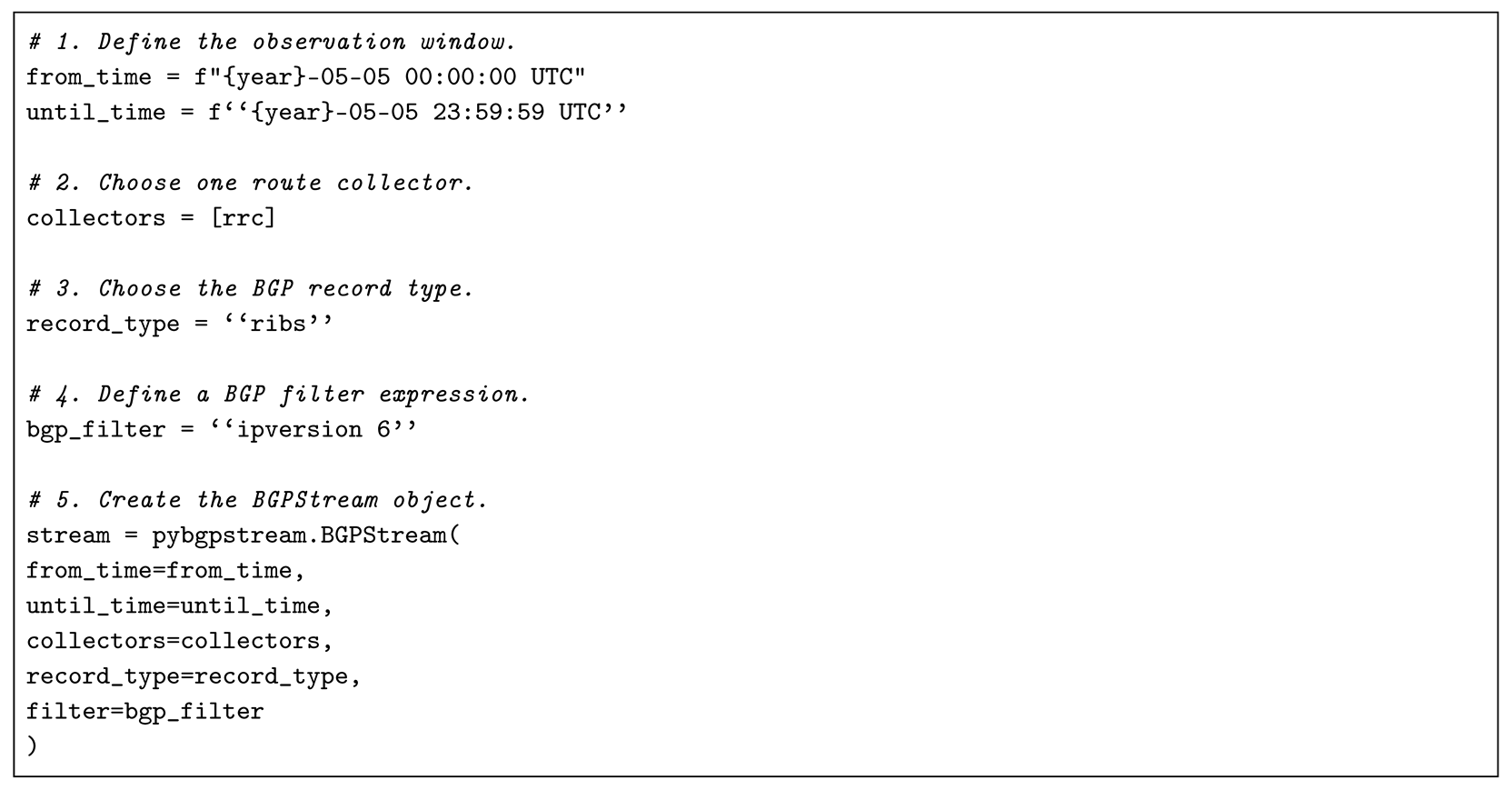 |
Table A1.
Guide to parameter values used in the pybgpstream RIPE RIS extraction—see Listing A1.
Appendix C.2. Collector Level Results
This subsection presents detailed results for each collector, including model selection, prediction errors, and comparisons between predicted and observed routing state.
For each collector, we report the best-fitting model selected by AIC in each fitting window, the associated prediction errors, and predicted versus observed prefix counts for each year in the prediction windows. This presentation allows assessment of model stability, out-of-sample error patterns, and cross-collector consistency. As each rolling backtest refits the model on a different training interval, the predictive equations are not identical across fitting windows. In that sense, the reported forecasts are piecewise: each fitting window yields its own fitted formula, and changes in the selected model family reflect changes in the apparent growth regime rather than merely changes in the forecast horizon. To make this explicit, predicted versus observed values are reported below in separate tables for each fitting window.
Appendix C.2.1. RRC03
Table A2 summarises the best-fitting model family and prediction errors across the four rolling backtest configurations.
Table A2.
The best-fitting model and prediction errors for RRC03 across rolling backtests.
Model selection at RRC03 shifts from stretched-exponential behaviour in the earliest fitting window to Richards behaviour in the longest fitting window. In the latest configuration, the prediction MAPE is 4.32 per cent, indicating the scale of relative forecasting error over the years 2023–2025.
Table A3.
Predicted versus observed prefix counts for RRC03, fitted on 2010–2015 with SE and evaluated on 2016–2020 (W1). APE denotes absolute percentage error.
Table A4.
Predicted versus observed prefix counts for RRC03, fitted on 2010–2017 with SE and evaluated on 2018–2022 (W2). APE denotes absolute percentage error.
Table A5.
Predicted versus observed prefix counts for RRC03, fitted on 2010–2020 with SE and evaluated on 2021–2025 (W3). APE denotes absolute percentage error.
Figure A1.
RRC03 observed prefix counts with fitted models for the 2010–2022 fitting window, with forecasts for 2023–2025 (W4).
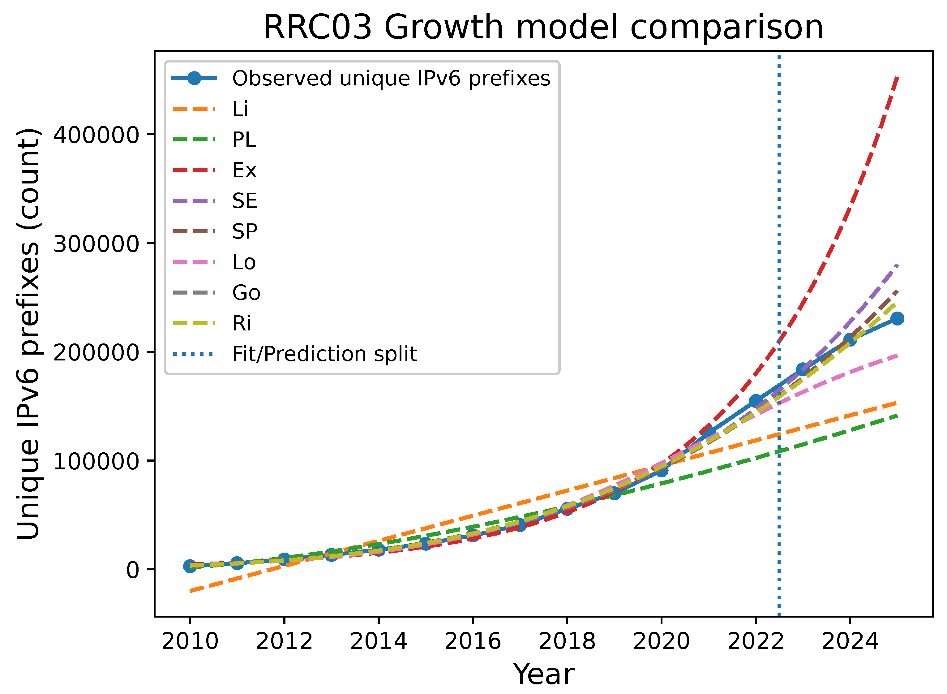
Table A6.
Predicted versus observed prefix counts for RRC03, fitted on 2010–2022 with Ri and evaluated on 2023–2025 (W4). APE denotes absolute percentage error.
Figure A2.
RRC03 residual diagnostics for the best-fitting model in the 2010–2022 fitting window. The left panel shows absolute residuals. The right panel shows relative residuals.
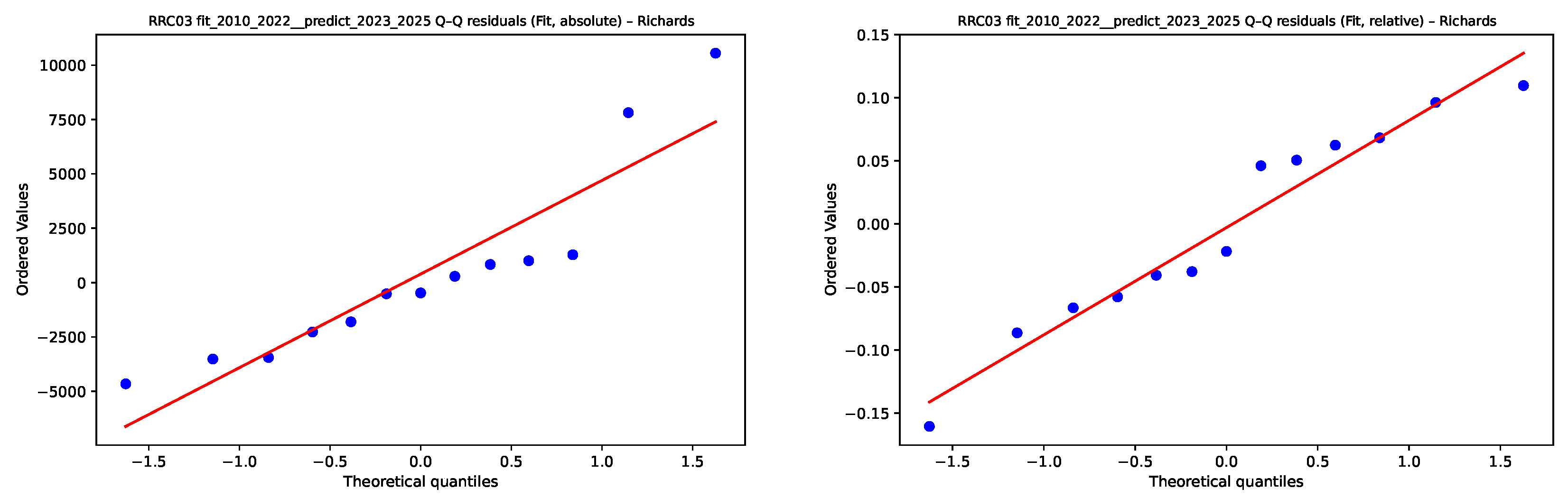
Appendix C.2.2. RRC06
Table A7 summarises the best-fitting model family and prediction errors across the four rolling backtest configurations.
Model selection at RRC06 shifts from linear behaviour in the earliest fitting window to Gompertz behaviour in the longest fitting window. In the latest configuration, the prediction MAPE is 7.94 per cent, indicating the scale of relative forecasting error over the years 2023–2025.
Table A7.
The best-fitting model and prediction errors for RRC06 across rolling backtests.
Table A8.
Predicted versus observed prefix counts for RRC06, fitted on 2010–2015 with Li and evaluated on 2016–2020 (W1). APE denotes absolute percentage error.
Table A9.
Predicted versus observed prefix counts for RRC06, fitted on 2010–2017 with Ex and evaluated on 2018–2022 (W2). APE denotes absolute percentage error.
Table A10.
Predicted versus observed prefix counts for RRC06, fitted on 2010–2020 with Go and evaluated on 2021–2025 (W3). APE denotes absolute percentage error.
Table A11.
Predicted versus observed prefix counts for RRC06, fitted on 2010–2022 with Go and evaluated on 2023–2025 (W4). APE denotes absolute percentage error.
Figure A3.
RRC06 observed prefix counts with fitted models for the 2010–2022 fitting window, with forecasts for 2023–2025 (W4).
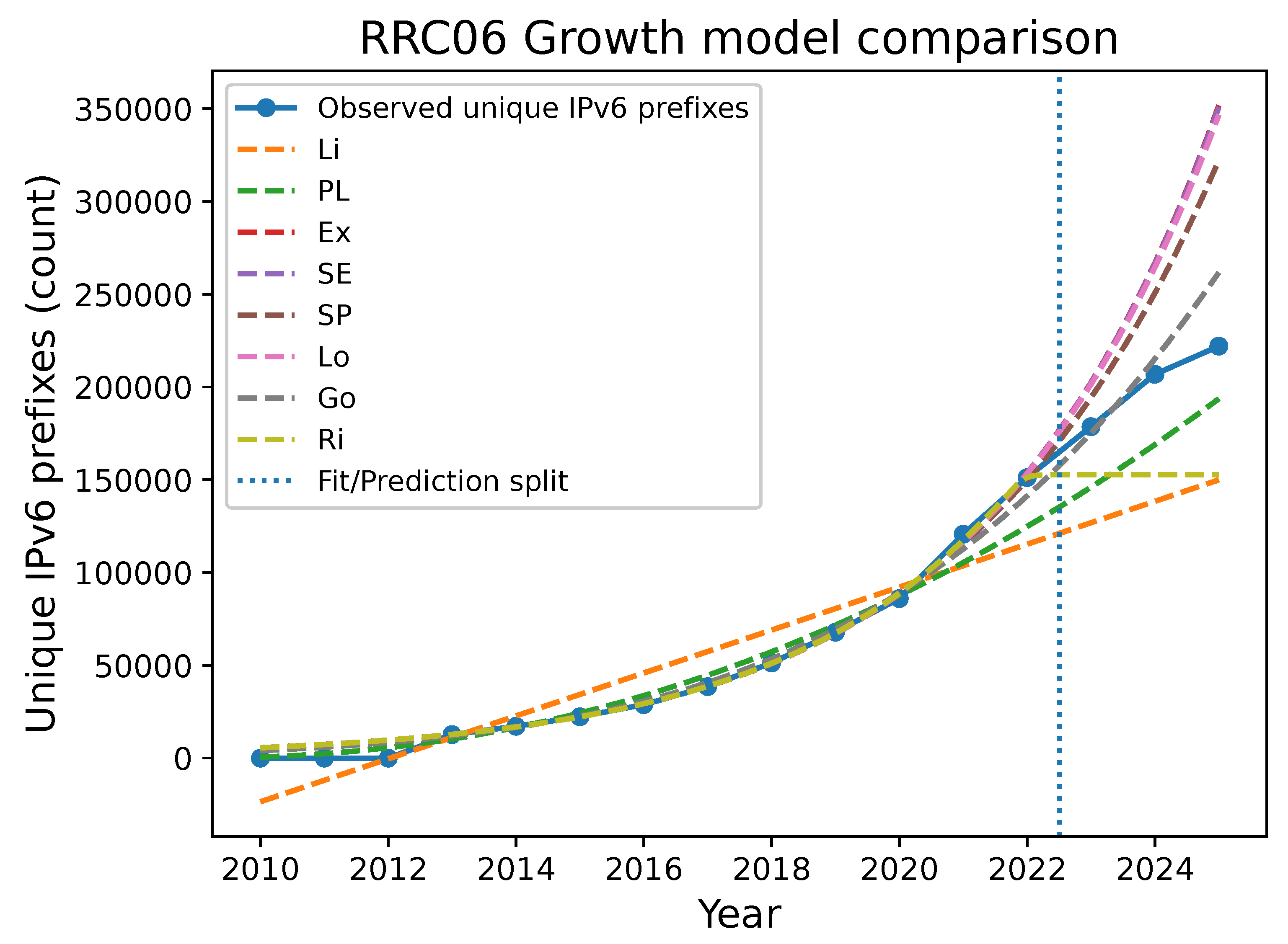
Figure A4.
RRC06 residual diagnostics for the best-fitting model in the 2010–2022 fitting window. The left panel shows absolute residuals. The right panel shows relative residuals.
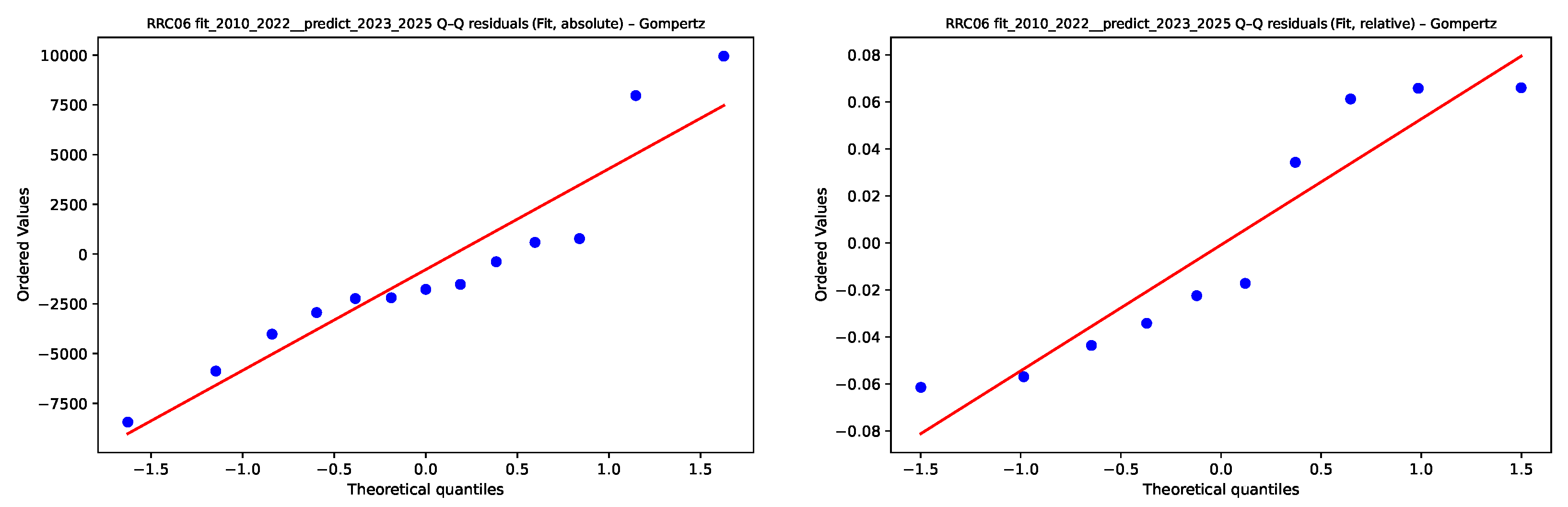
Appendix C.2.3. RRC11
Table A12 summarises the best-fitting model family and prediction errors across the four rolling backtest configurations.
Table A12.
The best-fitting model and prediction errors for RRC11 across rolling backtests.
Model selection at RRC11 shifts from stretched-exponential behaviour in the earliest fitting window to Richards behaviour in the longest fitting window. In the latest configuration, the prediction MAPE is 5.01 per cent, indicating the scale of relative forecasting error over the years 2023–2025.
Table A13.
Predicted versus observed prefix counts for RRC11, fitted on 2010–2015 with SE and evaluated on 2016–2020 (W1). APE denotes absolute percentage error.
Table A14.
Predicted versus observed prefix counts for RRC11, fitted on 2010–2017 with SE and evaluated on 2018–2022 (W2). APE denotes absolute percentage error.
Table A15.
Predicted versus observed prefix counts for RRC11, fitted on 2010–2020 with SE and evaluated on 2021–2025 (W3). APE denotes absolute percentage error.
Figure A5.
RRC11 observed prefix counts with fitted models for the 2010–2022 fitting window, with forecasts for 2023–2025 (W4).
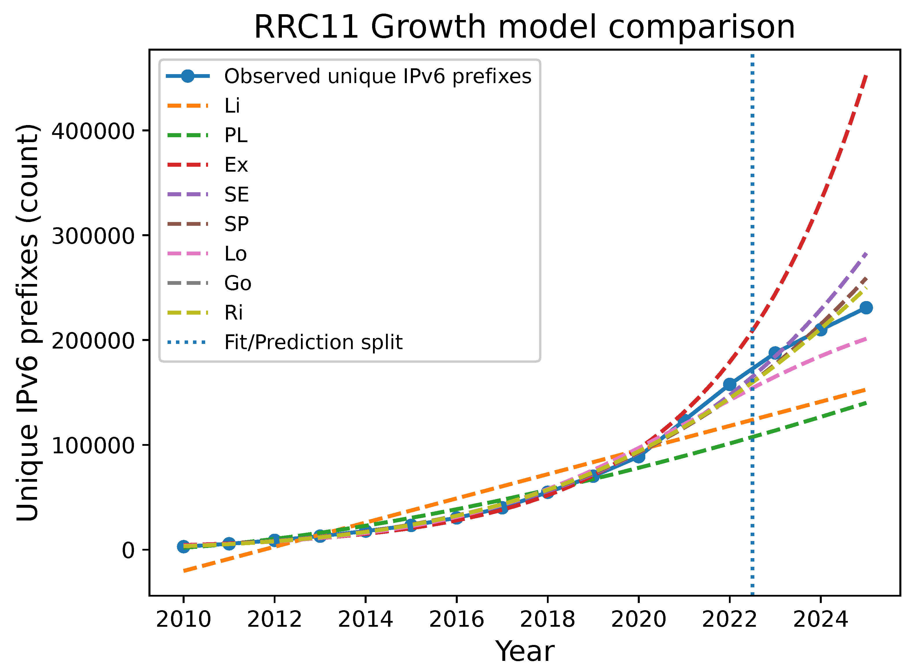
Figure A6.
RRC11 residual diagnostics for the best-fitting model in the 2010–2022 fitting window. The left panel shows absolute residuals. The right panel shows relative residuals.
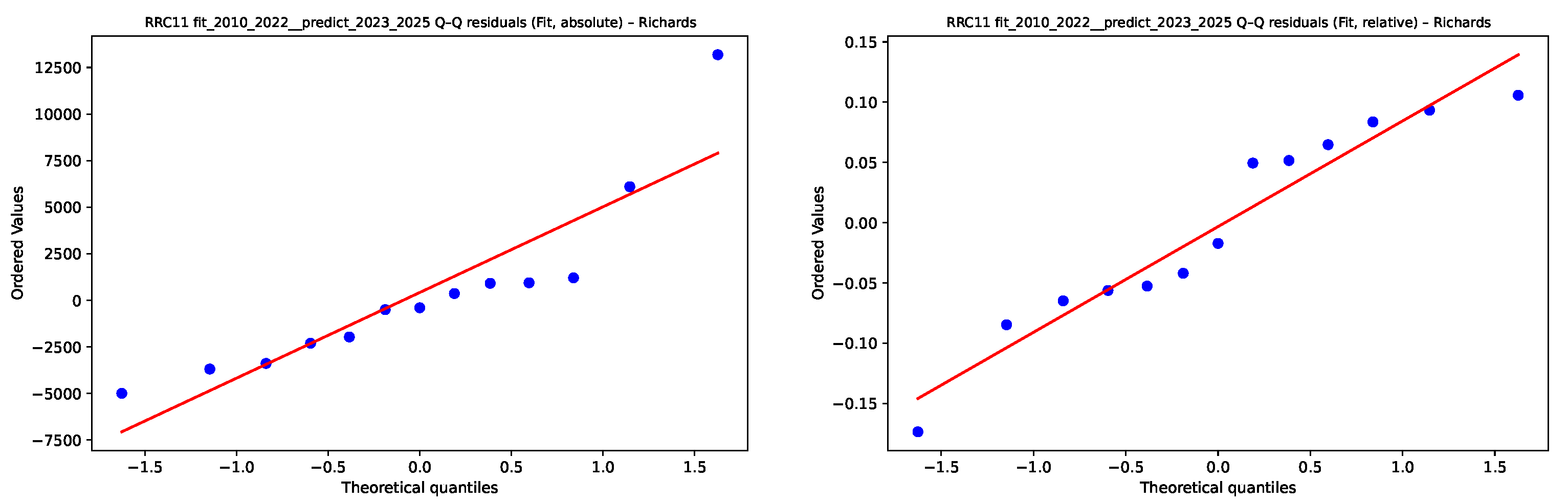
Table A16.
Predicted versus observed prefix counts for RRC11, fitted on 2010–2022 with Ri and evaluated on 2023–2025 (W4). APE denotes absolute percentage error.
Appendix C.2.4. RRC12
Table A17 summarises the best-fitting model family and prediction errors across the four rolling backtest configurations.
Table A17.
The best-fitting model and prediction errors for RRC12 across rolling backtests.
Model selection at RRC12 shifts from stretched-exponential behaviour in the earliest fitting window to Richards behaviour in the longest fitting window. In the latest configuration, the prediction MAPE is 4.65 per cent, indicating the scale of relative forecasting error over the years 2023–2025.
Table A18.
Predicted versus observed prefix counts for RRC12, fitted on 2010–2015 with SE and evaluated on 2016–2020 (W1). APE denotes absolute percentage error.
Table A19.
Predicted versus observed prefix counts for RRC12, fitted on 2010–2017 with SE and evaluated on 2018–2022 (W2). APE denotes absolute percentage error.
Table A20.
Predicted versus observed prefix counts for RRC12, fitted on 2010–2020 with SE and evaluated on 2021–2025 (W3). APE denotes absolute percentage error.
Table A21.
Predicted versus observed prefix counts for RRC12, fitted on 2010–2022 with Ri and evaluated on 2023–2025 (W4). APE denotes absolute percentage error.
Figure A7.
RRC12 observed prefix counts with fitted models for the 2010–2022 fitting window, with forecasts for 2023–2025 (W4).
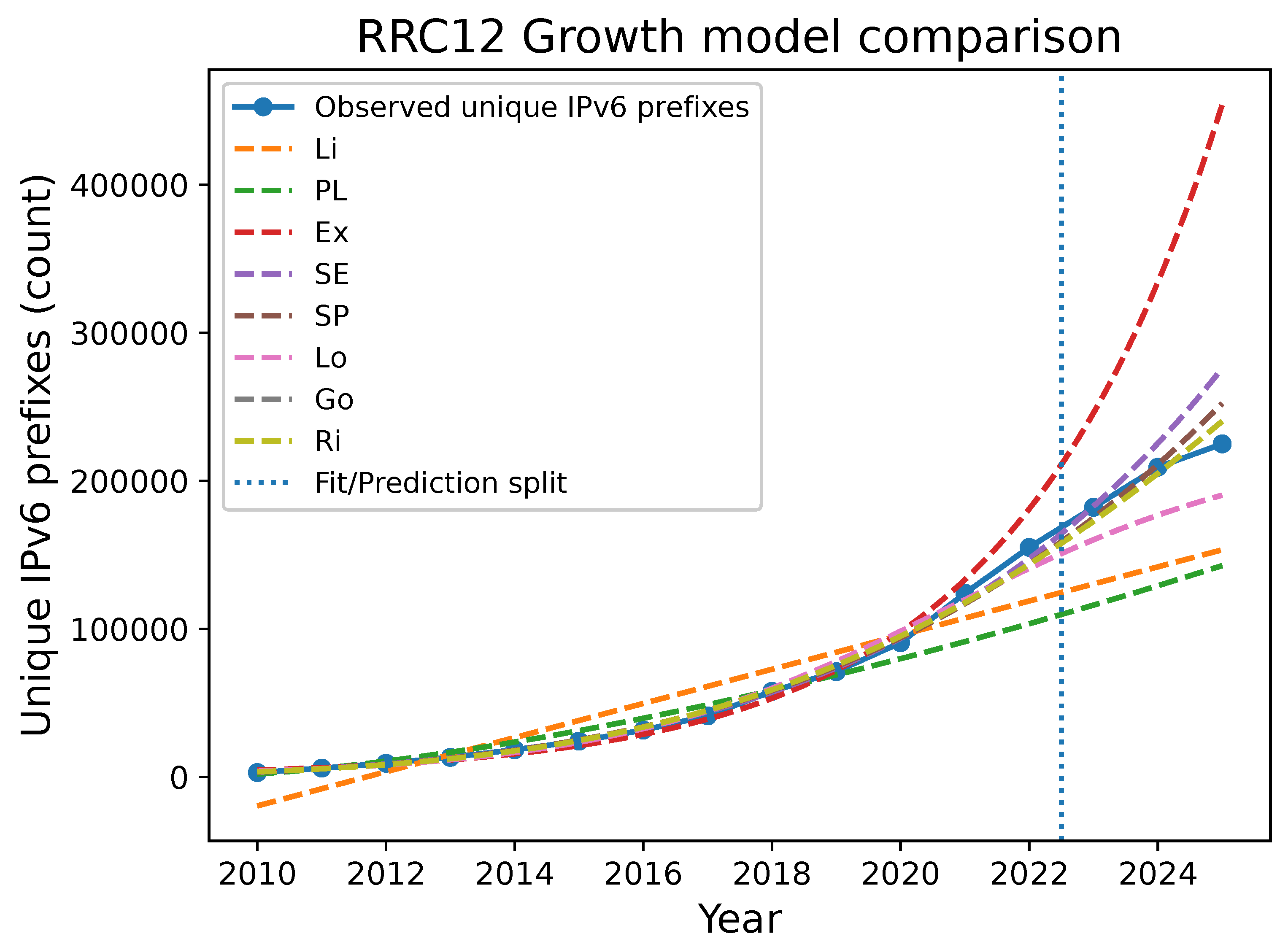
Figure A8.
RRC12 residual diagnostics for the best-fitting model in the 2010–2022 fitting window. The left panel shows absolute residuals. The right panel shows relative residuals.
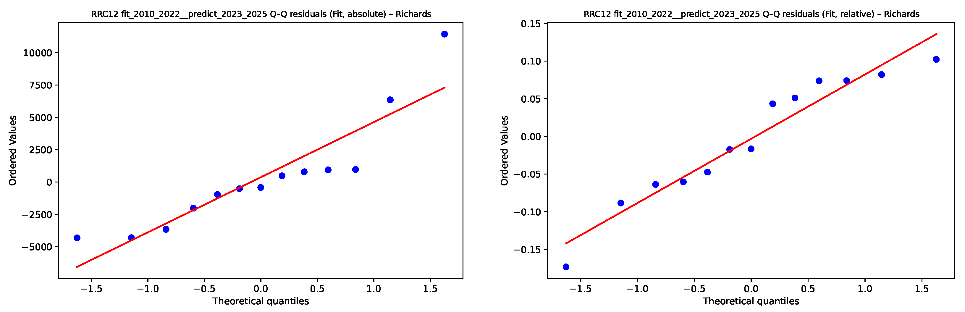
Appendix C.2.5. RRC13
Table A22 summarises the best-fitting model family and prediction errors across the four rolling backtest configurations.
Table A22.
The best-fitting model and prediction errors for RRC13 across rolling backtests.
Model selection at RRC13 shifts from stretched-exponential behaviour in the earliest fitting window to logistic behaviour in the longest fitting window. In the latest configuration, the prediction MAPE is 5.70 per cent, indicating the scale of relative forecasting error over the years 2023–2025.
Table A23.
Predicted versus observed prefix counts for RRC13, fitted on 2010–2015 with SE and evaluated on 2016–2020 (W1). APE denotes absolute percentage error.
Table A24.
Predicted versus observed prefix counts for RRC13, fitted on 2010–2017 with Ex and evaluated on 2018–2022 (W2). APE denotes absolute percentage error.
Table A25.
Predicted versus observed prefix counts for RRC13, fitted on 2010–2020 with SP and evaluated on 2021–2025 (W3). APE denotes absolute percentage error.
Table A26.
Predicted versus observed prefix counts for RRC13, fitted on 2010–2022 with Lo and evaluated on 2023–2025 (W4). APE denotes absolute percentage error.
Figure A9.
RRC13 observed prefix counts with fitted models for the 2010–2022 fitting window, with forecasts for 2023–2025 (W4).
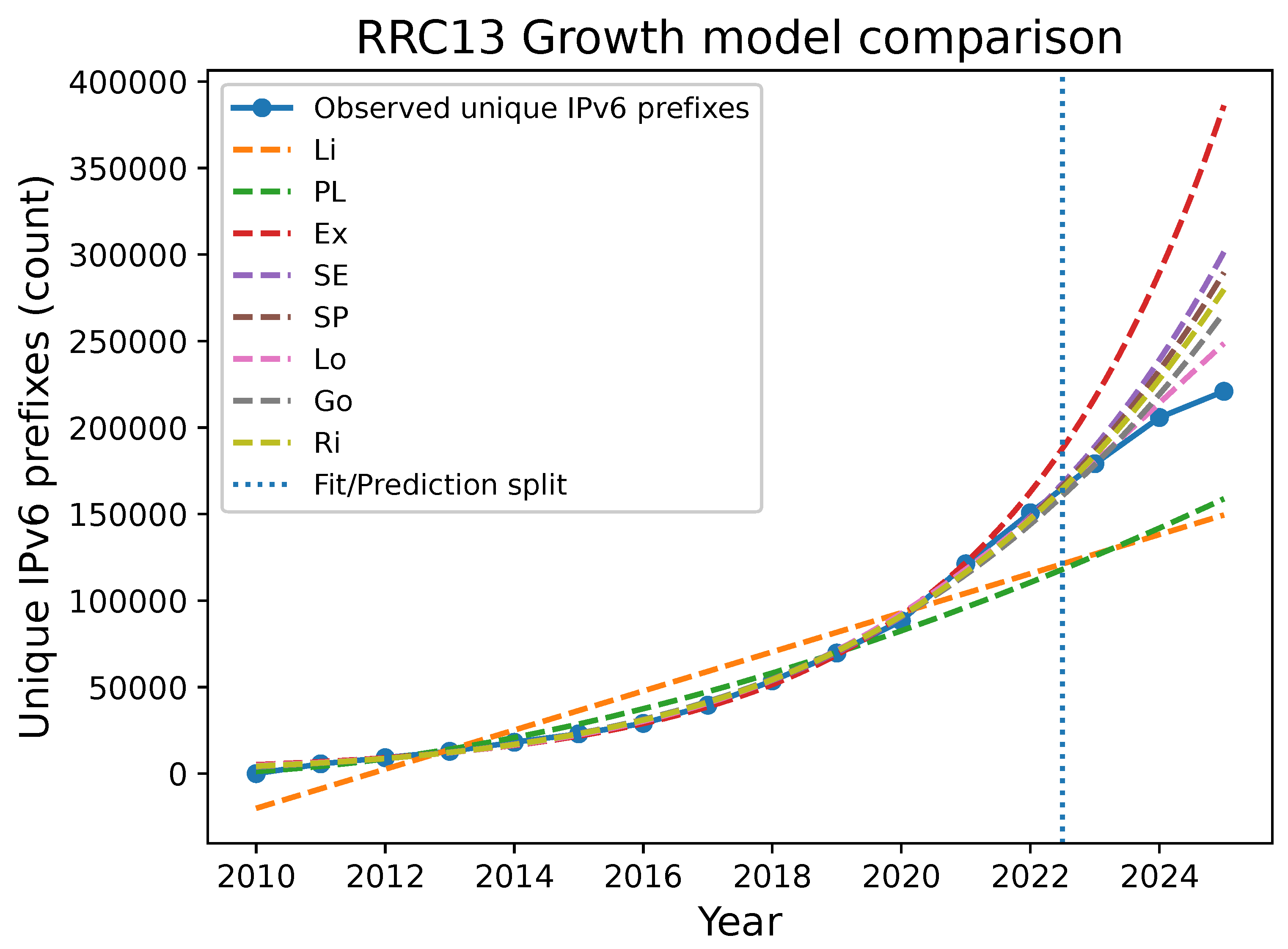
Figure A10.
RRC13 residual diagnostics for the best-fitting model in the 2010–2022 fitting window. The left panel shows absolute residuals. The right panel shows relative residuals.
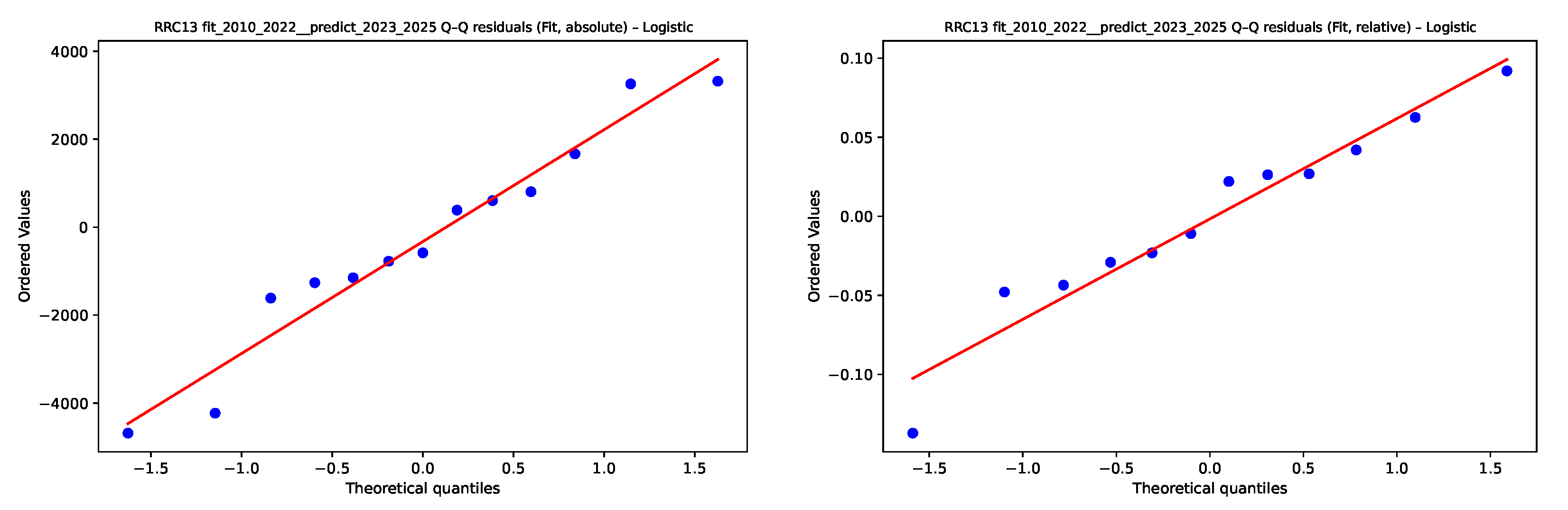
Appendix C.2.6. RRC14
Table A27 summarises the best-fitting model family and prediction errors across the four rolling backtest configurations.
Table A27.
The best-fitting model and prediction errors for RRC14 across rolling backtests.
Model selection at RRC14 shifts from stretched-exponential behaviour in the earliest fitting window to Richards behaviour in the longest fitting window. In the latest configuration, the prediction MAPE is 7.53 per cent, indicating the scale of relative forecasting error over the years 2023–2025.
Table A28.
Predicted versus observed prefix counts for RRC14, fitted on 2010–2015 with SE and evaluated on 2016–2020 (W1). APE denotes absolute percentage error.
Table A29.
Predicted versus observed prefix counts for RRC14, fitted on 2010–2017 with SE and evaluated on 2018–2022 (W2). APE denotes absolute percentage error.
Figure A11.
RRC14 observed prefix counts with fitted models for the 2010–2022 fitting window, with forecasts for 2023–2025 (W4).
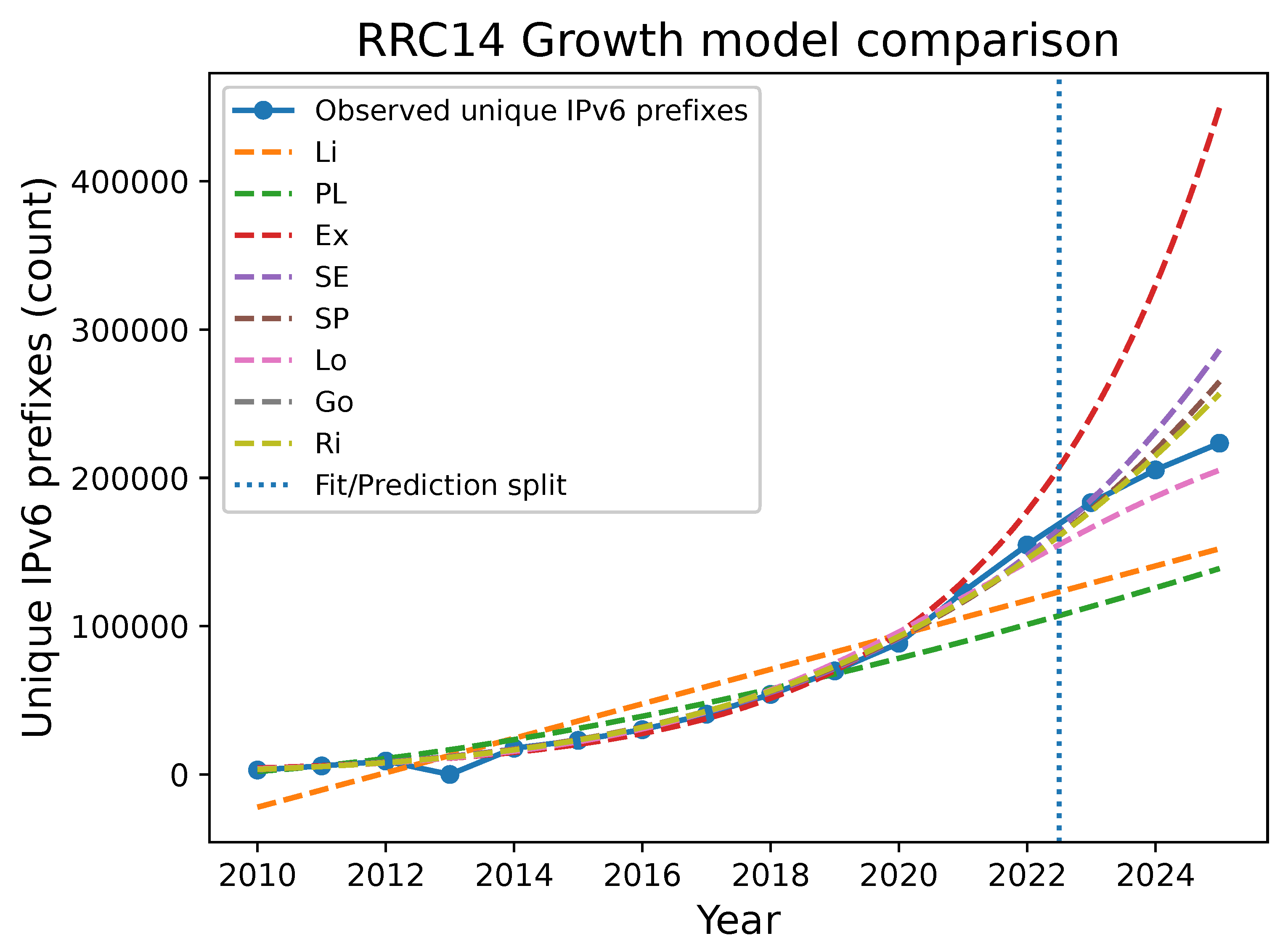
Table A30.
Predicted versus observed prefix counts for RRC14, fitted on 2010–2020 with SE and evaluated on 2021–2025 (W3). APE denotes absolute percentage error.
Table A31.
Predicted versus observed prefix counts for RRC14, fitted on 2010–2022 with Ri and evaluated on 2023–2025 (W4). APE denotes absolute percentage error.
Figure A12.
RRC14 residual diagnostics for the best-fitting model in the 2010–2022 fitting window. The left panel shows absolute residuals. The right panel shows relative residuals.
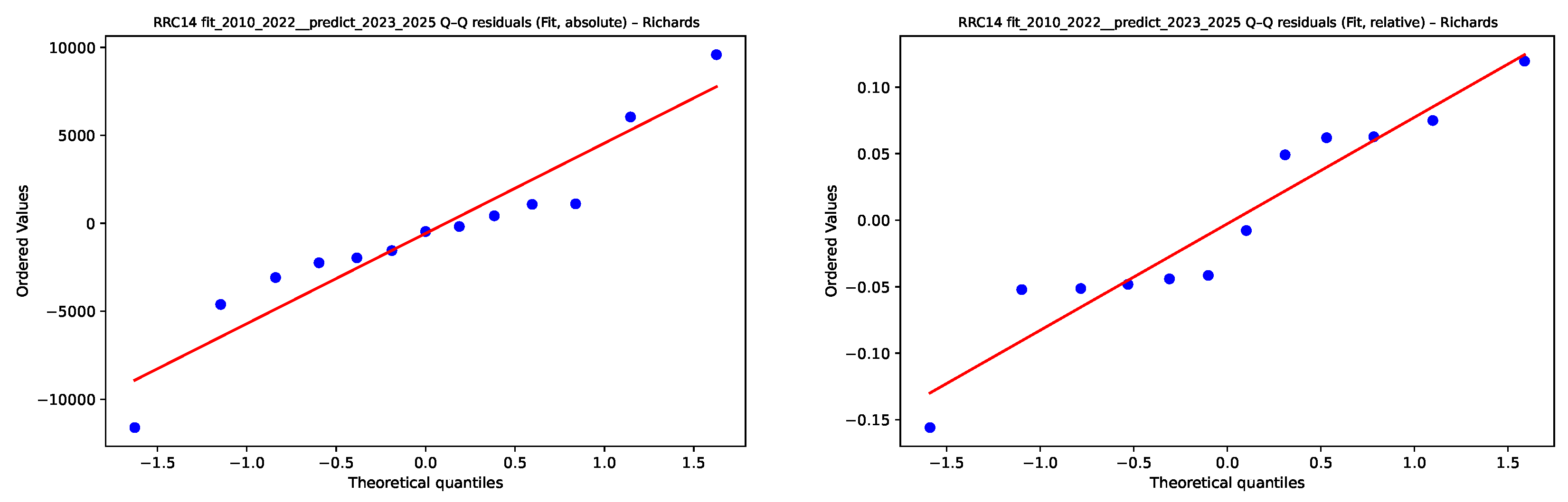
References
- Willinger, W.; Govindan, R.; Jamin, S.; Paxson, V.; Shenker, S. Scaling Phenomena in the Internet: Critically Examining Criticality. Proc. Natl. Acad. Sci. USA 2002, 99, 2573–2580. [Google Scholar] [CrossRef] [Scilit] [PubMed]
- Clauset, A.; Shalizi, C.R.; Newman, M.E.J. Power-Law Distributions in Empirical Data. SIAM Rev. 2009, 51, 661–703. [Google Scholar] [CrossRef] [Scilit]
- Labovitz, C.; Ahuja, A.; Bose, A.; Jahanian, F. Delayed Internet Routing Convergence. In Proceedings of the ACM SIGCOMM Conference, Stockholm, Sweden, 28 August–1 September 2000; pp. 175–187. [Google Scholar] [CrossRef] [Scilit]
- Huston, G. Analyzing the Internet’s BGP Routing Table. 2001. Available online: https://www.potaroo.net/papers/2001-3-bgptable/4-1-bgp.pdf (accessed on 5 February 2026).
- Huston, G. BGP in 2008. 2009. Available online: https://www.potaroo.net/ispcol/2009-03/bgp2008.pdf (accessed on 5 February 2026).
- Fuller, V.; Li, T.; Varadhan, K.; Yu, J. Classless Inter-Domain Routing (CIDR): An Address Assignment and Aggregation Strategy; RFC 1519 (PS); Internet Engineering Task Force: Wilmington, DE, USA, 1993. [Google Scholar] [CrossRef] [Scilit]
- Narten, T.; Huston, G.; Roberts, L. IPv6 Address Assignment to End Sites; RFC 6177(BCP); Internet Engineering Task Force: Wilmington, DE, USA, 2011. [Google Scholar] [CrossRef] [Scilit]
- Baker, F.; Bowers, C.; Linkova, J. Enterprise Multihoming Using Provider-Assigned IPv6 Addresses Without Network Prefix Translation: Requirements and Solutions; RFC 8678(I); Internet Engineering Task Force: Fremont, CA, USA, 2019. [Google Scholar] [CrossRef] [Scilit]
- Czyz, J.; Allman, M.; Zhang, J.; Iekel-Johnson, S.; Osterweil, E.; Bailey, M. Measuring IPv6 Adoption. In Proceedings of the 2014 ACM Conference on SIGCOMM, Chicago, IL, USA, 17–22 August 2014; pp. 87–98. [Google Scholar] [CrossRef] [Scilit]
- Dhamdhere, A.; Luckie, M.J.; Huffaker, B.; claffy, k.; Elmokashfi, A.; Aben, E. Measuring the Deployment of IPv6: Topology, Routing and Performance. In Proceedings of the 2012 Internet Measurement Conference, Boston, MA, USA, 14–16 November 2012; pp. 537–550. [Google Scholar] [CrossRef] [Scilit]
- RIPE NCC. RIPE Routing Information Service (RIS). 2024. Available online: https://ris.ripe.net/ (accessed on 5 February 2026).
- University of Oregon Route Views Project. Route Views Project. 2024. Available online: https://www.routeviews.org/ (accessed on 5 February 2026).
- Darwich, O.; Pelsser, C.; Vermeulen, K. Detecting Traffic Engineering from Public BGP Data. In Proceedings of the Passive and Active Measurement; Lecture Notes in Computer Science; Springer: Cham, Switzerland, 2025; Volume 15567, pp. 307–334. [Google Scholar] [CrossRef] [Scilit]
- Xygkou, I.M.; Chariton, A.A.; Dimitropoulos, X.A.; Dainotti, A. A First Look into Long-lived BGP Zombies. In Proceedings of the IMC ’25: 2025 ACM Internet Measurement Conference, New York, NY, USA, 28–31 October 2025; pp. 826–834. [Google Scholar] [CrossRef] [Scilit]
- Faloutsos, M.; Faloutsos, P.; Faloutsos, C. On Power-Law Relationships of the Internet Topology. In Proceedings of the ACM SIGCOMM Conference, Cambridge, MA, USA, 30 August 1999; pp. 251–262. [Google Scholar] [CrossRef] [Scilit]
- Laherrère, J.; Sornette, D. Stretched exponential distributions in nature and economy: Fat tails with characteristic scales. Eur. Phys. J. B 1998, 2, 525–539. [Google Scholar] [CrossRef] [Scilit]
- West, G.B.; Brown, J.H.; Enquist, B.J. A General Model for the Origin of Allometric Scaling Laws in Biology. Science 1997, 276, 122–126. [Google Scholar] [CrossRef] [Scilit] [PubMed]
- Rogers, E.M. Diffusion of Innovations, 5th ed.; Free Press: New York, NY, USA, 2003. [Google Scholar]
- Bush, R.; Meyer, D. Some Internet Architectural Guidelines and Philosophy; RFC 3439(I); Internet Engineering Task Force: Wilmington, DE, USA, 2002. [Google Scholar] [CrossRef] [Scilit]
- Pastor-Satorras, R.; Vespignani, A. Evolution and Structure of the Internet: A Statistical Physics Approach; Cambridge University Press: Cambridge, UK, 2004. [Google Scholar] [CrossRef] [Scilit]
- Center for Applied Internet Data Analysis (CAIDA). The CAIDA Ark Internet Measurement Infrastructure. 2009. Available online: https://www.caida.org/projects/ark/ (accessed on 5 February 2026).
- Dhamdhere, A.; Dovrolis, C. Ten Years in the Evolution of the Internet Ecosystem. In Proceedings of the ACM Internet Measurement Conference, Vouliagmeni, Greece, 20–22 October 2008; pp. 183–196. [Google Scholar] [CrossRef] [Scilit]
- Oliveira, R.; Pei, D.; Willinger, W.; Zhang, B.; Zhang, L. The (In)Completeness of the Observed Internet AS-Level Structure. IEEE/ACM Trans. Netw. 2010, 18, 109–122. [Google Scholar] [CrossRef] [Scilit]
- Alfroy, T.; Holterbach, T.; Krenc, T.; Claffy, K.C.; Pelsser, C. The Next Generation of BGP Data Collection Platforms. In Proceedings of the ACM SIGCOMM ’24: ACM SIGCOMM 2024 Conference, Sydney, Australia, 4–8 August 2024; pp. 794–812. [Google Scholar] [CrossRef] [Scilit]
- Adamic, L.A.; Huberman, B.A. Zipf’s Law and the Internet. Glottometrics 2002, 3, 143–150. [Google Scholar]
- Solow, R.M. A Contribution to the Theory of Economic Growth. Q. J. Econ. 1956, 70, 65–94. [Google Scholar] [CrossRef] [Scilit]
- Arthur, W.B. Competing technologies, increasing returns, and lock-in by historical events. Econ. J. 1989, 99, 116–131. [Google Scholar] [CrossRef] [Scilit]
- Valapu, S.T.; Heidemann, J.S. Towards a Non-Binary View of IPv6 Adoption. In Proceedings of the IMC ’25: 2025 ACM Internet Measurement Conference, Madison, WI, USA, 28–31 October 2025; pp. 727–745. [Google Scholar] [CrossRef] [Scilit]
- Richter, P.; Wohlfart, F.; Vallina-Rodriguez, N.; Allman, M.; Bush, R.; Feldmann, A.; Kreibich, C.; Weaver, N.; Paxson, V. A Multi-Perspective Analysis of Carrier-Grade NAT Deployment. In Proceedings of the 2016 Internet Measurement Conference, Santa Monica, CA, USA, 14–16 November 2016; pp. 215–229. [Google Scholar] [CrossRef] [Scilit]
- Barabási, A.L.; Albert, R. Emergence of Scaling in Random Networks. Science 1999, 286, 509–512. [Google Scholar] [CrossRef] [Scilit] [PubMed]
- Bass, F.M. A New Product Growth Model for Consumer Durables. Manag. Sci. 1969, 15, 215–227. [Google Scholar] [CrossRef] [Scilit]
- Orsini, C.; King, A.; Giordano, D.; Giotsas, V.; Dainotti, A. BGPStream: A Software Framework for Live and Historical BGP Data Analysis. In Proceedings of the IMC ’16: 2016 Internet Measurement Conference, Santa Monica, CA, USA, 14–16 November 2016; pp. 429–444. [Google Scholar] [CrossRef] [Scilit]
- Fontugne, R.; Shah, A.; Aben, E. The (Thin) Bridges of AS Connectivity: Measuring Dependency Using AS Hegemony. In Passive and Active Measurement; Lecture Notes in Computer Science; Springer: Cham, Switzerland, 2018; Volume 10771, pp. 216–227. [Google Scholar] [CrossRef] [Scilit]
- Internet Society. World IPv6 Luanch Day; Internet Society: Reston, VA, USA, 2011. [Google Scholar]
- Google. Google IPv6 Statistics. 2010. Available online: https://www.google.com/intl/en/ipv6/statistics.html (accessed on 5 February 2026).
- Kohlrausch, R. Theorie des elektrischen R"uckstandes in der Leidener Flasche. Ann. Der Phys. Und Chem. 1854, 167, 179–214. [Google Scholar] [CrossRef] [Scilit]
- Williams, G.; Watts, D.C. Non-Symmetrical Dielectric Relaxation Behaviour Arising from a Simple Empirical Decay Function. Trans. Faraday Soc. 1970, 66, 80–85. [Google Scholar] [CrossRef] [Scilit]
- Verhulst, P.F. Notice sur la loi que la population poursuit dans son accroissement. Corresp. Mathématique Et Phys. 1838, 10, 113–121. [Google Scholar]
- Gompertz, B. On the Nature of the Function Expressive of the Law of Human Mortality. Philos. Trans. R. Soc. Lond. 1825, 115, 513–583. [Google Scholar] [CrossRef] [Scilit]
- Richards, F.J. A Flexible Growth Function for Empirical Use. J. Exp. Bot. 1959, 10, 290–301. [Google Scholar] [CrossRef] [Scilit]
- Akaike, H. A New Look at the Statistical Model Identification. IEEE Trans. Autom. Control 1974, 19, 716–723. [Google Scholar] [CrossRef] [Scilit]
- Burnham, K.P.; Anderson, D.R. Model Selection and Multimodel Inference: A Practical Information-Theoretic Approach; Springer: Berlin/Heidelberg, Germany, 2002. [Google Scholar] [CrossRef] [Scilit]
- Ravikumar, V.; Mahapatra, R. TCAM architecture for IP lookup using prefix properties. IEEE Micro 2004, 24, 60–69. [Google Scholar] [CrossRef] [Scilit]
- Kumar, S.; Jedhe, G.; Deshpande, C.; Gouoi, A.; Su, P.; Jway, K.S.; Seoh, T. A 3 nm FinFET 2.2 Gsearch/s 0.305 fJ/b TCAM with Dynamically Gated Search Lines for Data-Center ASICs. In Proceedings of the 2025 IEEE International Solid-State Circuits Conference (ISSCC); IEEE: Piscataway, NJ, USA, 2025; Volume 68, pp. 496–498. [Google Scholar] [CrossRef] [Scilit]
- Smith, L.; Lipner, I. Free Pool of IPv4 Address Space Depleted. 2011. Available online: https://www.nro.net/ipv4-free-pool-depleted/ (accessed on 5 February 2026).
- GSM Association. The Mobile Economy 2026; Technical report; The GSM Association (GSMA): London, UK, 2026; Available online: https://www.gsma.com/solutions-and-impact/connectivity-for-good/mobile-economy/ (accessed on 5 May 2026).
- Galego, N.M.C.; Pascoal, R.M.; Brand ao, P.R. IPv6 in IoT. In Proceedings of the Management, Tourism and Smart Technologies; Montenegro, C., Rocha, Á., Cueva Lovelle, J.M., Eds.; Springer Nature: Cham, Switzerland, 2024; pp. 89–94. [Google Scholar] [CrossRef] [Scilit]
- Internet Architetcure Board (IAB). IAB/IESG Recommendations on IPv6 Address Allocations to Sites; RFC 3177(I); Internet Society: Reston, VA, USA, 2001. [Google Scholar] [CrossRef] [Scilit]
- Ginsberg, L.; Decraene, B.; Litkowski, S.; Shakir, R. Segment Routing Architecture; Filsfils, C., Previdi, S., Eds.; RFC 8402(I); Internet Society: Reston, VA, USA, 2018. [Google Scholar] [CrossRef] [Scilit]
- Leddy, J.; Voyer, D.; Matsushima, S.; Li, Z. Segment Routing over IPv6 (SRv6) Network Programming; Filsfils, C., Previdi, S., Eds.; RFC 8986(PS); Internet Society: Reston, VA, USA, 2021. [Google Scholar] [CrossRef] [Scilit]
- Barreto, R.P.; Bertholdo, L.M.; Marcos, P.d.B. Routing Under Siege: How Traffic Engineering Decisions Facilitate Prefix Hijackings. In Proceedings of the Passive and Active Measurement; Lecture Notes in Computer Science; Springer: Cham, Switzerland, 2026; Volume 16477, pp. 44–70. [Google Scholar] [CrossRef] [Scilit]
- Snijders, J.; Maddison, B.; Lepinski, M.; Voyer, D.; Kong, D.; Kent, S. A Profile for Route Origin Authorizations (ROAs); RFC 9582(PS); Internet Society: Reston, VA, USA, 2024. [Google Scholar] [CrossRef] [Scilit]
- Lepinski, M.; Kent, S. An Infrastructure to Support Secure Internet Routing; RFC 6480(I); Internet Society: Reston, VA, USA, 2012. [Google Scholar] [CrossRef] [Scilit]
- Schulmann, H.; Vogel, N.; Waidner, M. Are We Actually There? Assessing RPKI Maturity. Commun. ACM 2026, 69, 80–91. [Google Scholar] [CrossRef] [Scilit]
- Ali, W.; Fang, C.; Khan, A. A survey on the state-of-the-art CDN architectures and future directions. J. Netw. Comput. Appl. 2025, 236, 104106. [Google Scholar] [CrossRef] [Scilit]
- Barnardos, C.J.; Rahman, A.; Zuniga, J.C.; Contreras, L.M.; Aranda, P.; Lynch, P. Network Virtualization Research Challenges; RFC 8586(I); Internet Society: Reston, VA, USA, 2019. [Google Scholar] [CrossRef] [Scilit]
- Atkinson, R.; Bhatti, S.N. Identifier-Locator Network Protocol (ILNP) Architectural Description; RFC 6740(E); Internet Engineering Task Force: Wilmington, DE, USA, 2012. [Google Scholar] [CrossRef] [Scilit]
- Atkinson, R.; Bhatti, S.N. Identifier-Locator Network Protocol (ILNP) Engineering Considerations; RFC 6741(E); Internet Engineering Task Force: Wilmington, DE, USA, 2012. [Google Scholar] [CrossRef] [Scilit]
- Perron, P. Dealing with Structural Breaks. In Palgrave Handbook of Econometrics; Mills, T.C., Patterson, K., Eds.; Palgrave Macmillan: London, UK, 2006; pp. 278–352. [Google Scholar]
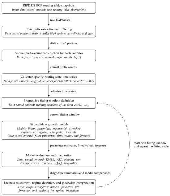
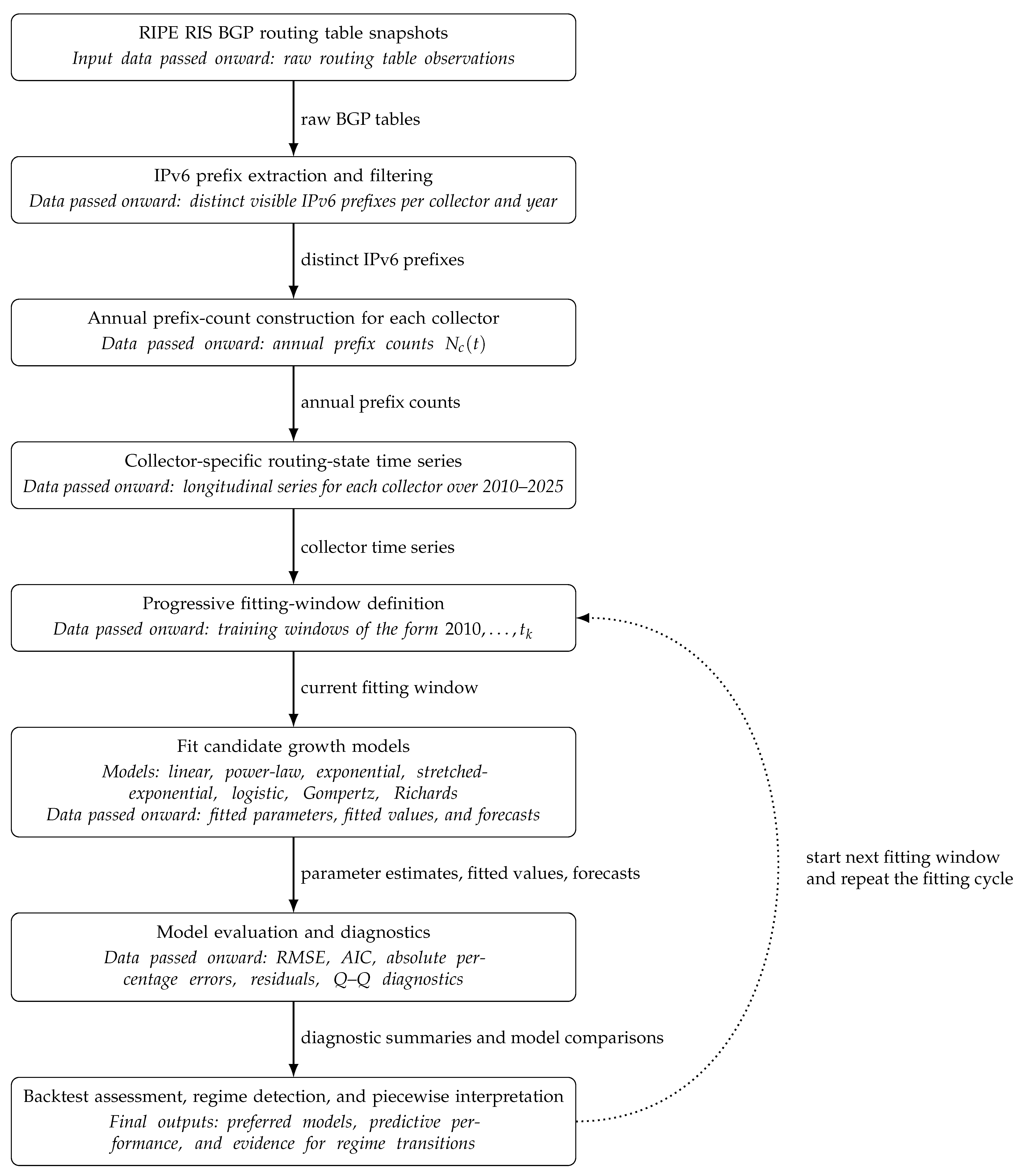
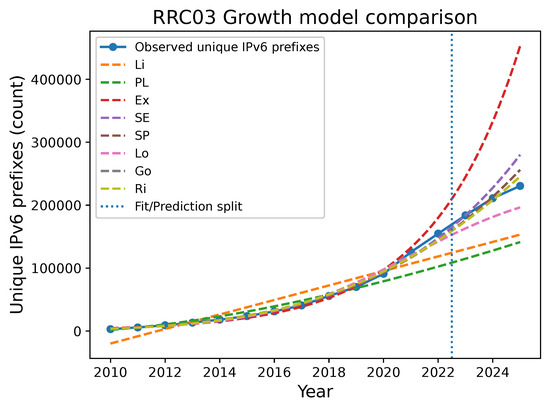
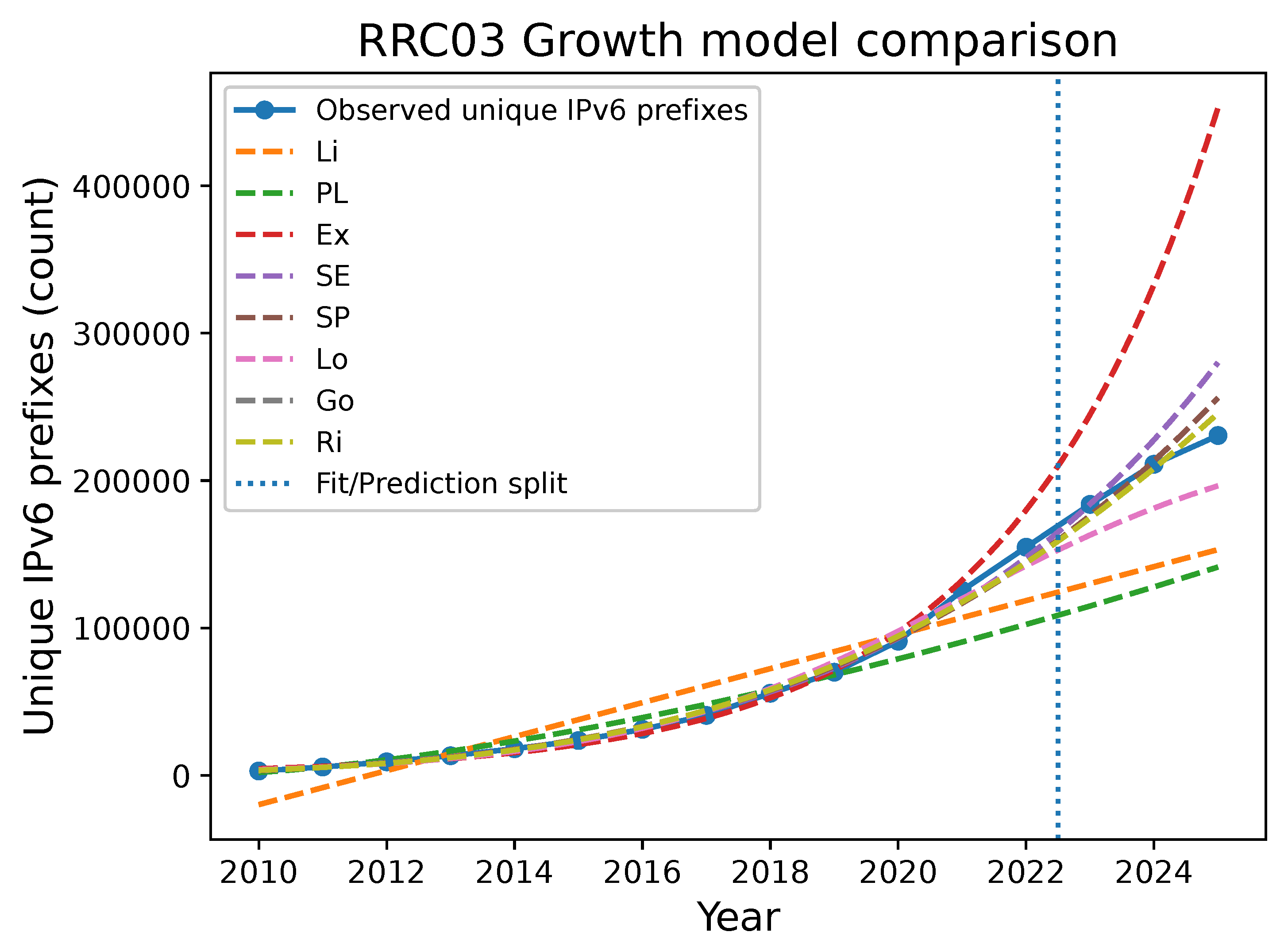
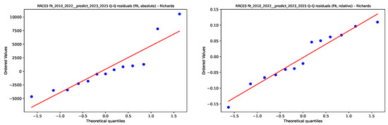
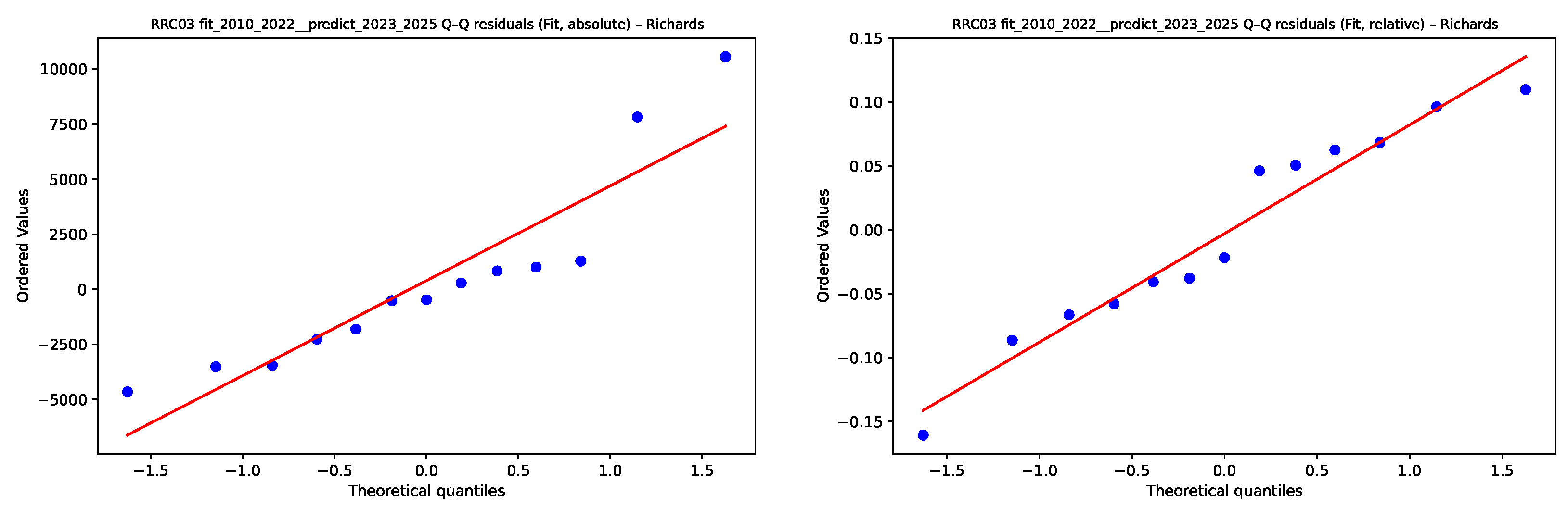

Disclaimer/Publisher’s Note: The statements, opinions and data contained in all publications are solely those of the individual author(s) and contributor(s) and not of MDPI and/or the editor(s). MDPI and/or the editor(s) disclaim responsibility for any injury to people or property resulting from any ideas, methods, instructions or products referred to in the content. |
© 2026 by the authors. Licensee MDPI, Basel, Switzerland. This article is an open access article distributed under the terms and conditions of the Creative Commons Attribution (CC BY) license.