Leveraging Neural Networks Trained with Scaled Conjugate Gradient for Enhanced VANET Performance in High-Mobility Environments

Abstract

Vehicular Ad Hoc Networks (VANETs) face significant challenges in high-mobility environments, where dynamic channel conditions, particularly Doppler Shift (DS), degrade communication reliability and increase latency, thereby undermining safety-critical applications. To address these limitations, this paper proposes a neural network (NN)-based link adaptation strategy trained using the Scaled Conjugate Gradient (SCG) algorithm. SCG is selected as a second-order approximation optimizer that leverages curvature information to produce well-conditioned weight updates particularly suited to the small, physics-constrained training dataset. The SCG-optimized model dynamically adjusts transmission parameters to mitigate DS effects, improving real-time adaptability by explicitly incorporating Doppler Shift as a key input feature. Simulation results demonstrate that the proposed approach outperforms both the conventional Auto Rate Fallback (ARF) method and the SampleRate baseline. Specifically, the SCG-based strategy achieves an overall throughput improvement of +34.6% relative to ARF (1.77 Mbps vs. 1.32 Mbps) across all tested conditions, with condition-specific gains of +16.1% at 5 Hz Doppler (0.9 km/h), +21.7% at 750 Hz (137.3 km/h), and +35.2% at 1500 Hz (274.6 km/h), while consistently reducing transmission duration. A formal ablation study confirms that the Doppler Shift feature alone contributes +67% to +78% throughput gain at high mobility (DS > 900 Hz) compared to an SNR-only model. The main contributions of this work are threefold: (i) the explicit integration of Doppler Shift as a first-class input feature for link adaptation; (ii) the application of SCG optimization for fast, stable training of a lightweight feedforward neural network on a compact, physics-constrained dataset; and (iii) the formal ablation study that isolates and quantifies the Doppler feature’s contribution, establishing that the performance gain is attributable to feature engineering rather than the neural network architecture alone. This approach offers a scalable, real-time solution for Doppler-resilient VANET link adaptation.

1. Introduction

Road traffic safety remains one of the most pressing global public health concerns. According to the World Health Organization (WHO), road traffic accidents account for approximately 1.19 million fatalities annually worldwide, with disproportionately severe social and economic consequences for younger and working-age populations [1]. This persistent burden has accelerated the development of Intelligent Transportation Systems (ITS), which aim to improve road safety, traffic efficiency, and environmental sustainability through advanced sensing, communication, and automation technologies. A core enabler of ITS is the Vehicular Ad Hoc Network (VANET), which supports direct communication among vehicles (V2V) and between vehicles and roadside infrastructure (V2I). Standardized within the Wireless Access in Vehicular Environments (WAVE) or Dedicated Short-Range Communications (DSRC) framework, VANETs provide the communication substrate for a wide range of applications, from cooperative safety services to traffic management and infotainment systems [2,3,4,5].

The effectiveness of VANET-based applications depends critically on the reliable and timely dissemination of information. Periodic Cooperative Awareness Messages (CAMs) enable vehicles to maintain shared situational awareness by broadcasting dynamic state information such as position, velocity, and heading [6]. Event-driven Decentralized Environmental Notification Messages (DENMs) convey urgent hazard warnings and impose stringent latency and reliability requirements [7]. Meeting these performance demands consistently remains challenging in real-world deployments, where communication links are subject to rapid fluctuations and strict timing constraints.

Among channel impairments, Doppler Shift (DS) plays a particularly detrimental role, as it disrupts the orthogonality of subcarriers in OFDM-based systems such as IEEE 802.11p, leading to inter-carrier interference (ICI), elevated packet error rates, and unstable link performance [8,9]. Additional effects such as shadowing, multipath fading, and variable traffic density further exacerbate channel volatility [10,11]. Traditional rate adaptation algorithms were not designed to anticipate Doppler-induced degradation, nor to react effectively within the short coherence times typical of high-speed vehicular channels. Recent advances in machine learning (ML) offer a promising pathway toward such intelligent adaptation [12].

Motivated by this perspective, this paper introduces a Doppler-aware link adaptation framework based on a neural network (NN) optimized using the Scaled Conjugate Gradient (SCG) algorithm. The selection of SCG is not arbitrary: recent work by Bajaj et al. [13] demonstrates that stability in weight updates is a critical factor for reliable learning in physics-constrained problems with small, non-stationary datasets, a finding that applies directly to VANET link adaptation, where the training dataset contains 120 samples governed by IEEE 802.11p physical constraints and the channel statistics are non-stationary across mobility regimes. SCG’s second-order curvature information produces monotonically stable updates that are better conditioned than first-order methods (SGD, Adam) under these constraints.

This work makes three distinct and differentiated contributions to the field of ML-based link adaptation in vehicular networks. First, we introduce a joint Doppler-SNR input representation for MCS selection that enables anticipatory adaptation to mobility-induced channel degradation rather than reactive adaptation to observed packet outcomes. Existing rate adaptation algorithms, including ARF [14], SampleRate [15], and Minstrel [16] are reactive: they adjust the MCS only after observing packet success or failure events. This introduces an inherent latency between channel degradation and rate adjustment that is particularly damaging in high-mobility VANET scenarios where the channel coherence time Tc is shorter than the reaction cycle of these algorithms. Second, the proposed method is trained on the VANET-LA dataset, which provides synchronized per-packet PHY-layer measurements (SNR, Doppler Shift, MCS index) under urban NLOS conditions aligned with IEEE 802.11p. The absence of such a dataset has been the primary obstacle to ML-based link adaptation research in VANETs [2,17]. Third, a formal ablation study isolates and quantifies the Doppler feature’s contribution: at DS > 900 Hz, the joint SNR+Doppler model achieves 60–80% higher throughput than an SNR-only model with identical architecture and training procedure. This result directly demonstrates that the performance gain is attributable to the feature engineering choice and not merely to the use of a neural network which constitutes the core scientific claim of this work.

The remainder of this paper is organized as follows. Section 2 reviews related work. Section 3 presents the mathematical analysis of Doppler Shift. Section 4 describes the proposed neural network architecture. Section 5 details the SCG optimization algorithm. Section 6 outlines the experimental setup and results. Section 7 concludes the paper.

2. Related Works

Link adaptation (LA) and rate adaptation (RA) play a pivotal role in ensuring reliable, spectrally efficient, and low-latency communication in VANETs, where wireless links are subject to extreme mobility, frequent topology changes, and stringent QoS requirements [18]. Unlike conventional wireless networks, VANET channels exhibit rapid time selectivity, short coherence times, and pronounced Doppler effects, which significantly complicate reliable MCS selection.

Several rate adaptation algorithms have been proposed for IEEE 802.11 networks, and their applicability to the IEEE 802.11p vehicular context requires careful examination. The Auto Rate Fallback (ARF) algorithm [14] adjusts the MCS by incrementing after 10 consecutive successes and decrementing after 2 consecutive failures. While simple and widely implemented, ARF is a purely reactive algorithm: it responds to observed outcomes rather than anticipating channel conditions, making it slow to adapt under the rapid channel variations characteristic of high-mobility VANET scenarios. The SampleRate algorithm [15] improves on ARF by periodically probing higher MCS levels to estimate their current viability, maintaining a per-MCS success rate table. SampleRate has been shown to outperform ARF in infrastructure WLANs and serves as a stronger baseline for vehicular comparison.

The Minstrel algorithm [16] and its multi-stream extension Minstrel-HT were designed for 802.11n/ac infrastructure networks and exploit channel reciprocity and ACK-based feedback mechanisms that do not hold reliably in V2V NLOS scenarios under high mobility and asymmetric link conditions. Furthermore, Minstrel-HT’s probing strategy assumes relatively stable channel statistics over the probing interval, an assumption violated in urban NLOS environments where coherence times fall below 1 ms at vehicle speeds above 130 km/h (i.e., DS > 709 Hz at 5.9 GHz). The RRAA [19] and RBAR algorithms require per-packet RTS/CTS overhead that is architecturally incompatible with the broadcast-dominated communication pattern of IEEE 802.11p safety messages (CAM/DENM), where unicast acknowledgement mechanisms are not available [20]. For these reasons, ARF and SampleRate are selected as the primary baselines in this work.

Data-driven and context-aware adaptation strategies have gained significant traction. Supervised learning approaches have demonstrated that neural networks can effectively learn complex, nonlinear mappings between channel conditions and optimal transmission parameters [21]. In the context of Cellular V2X (C-V2X), Rokoni et al. [22] addressed the practical limitation of absent or delayed feedback in Mode 4 sidelink communication by training gradient boosting models and neural networks on large-scale real-world urban driving datasets. Banerjee et al. [23] incorporated CSI alongside contextual information such as vehicle speed, GPS-derived location, and estimated inter-cell interference, employing ensembles of deep RL agents to jointly optimize MCS and transmit power. Zhang and Wang [24] proposed a Context-Aware Resource Allocation (CARA) scheme that embeds collision risk into the allocation process through a non-cooperative game formulation, prioritizing high-risk vehicles to enhance the reliability and latency of safety-critical messages.

Despite these advances, several critical gaps remain. First, the majority of existing ML-based schemes rely primarily on SNR or aggregated channel quality indicators, rarely incorporating Doppler Shift explicitly as a first-class input feature. This omission limits the ability of learning models to anticipate Doppler-induced degradation within the short coherence times characteristic of high-speed vehicular channels. Second, although sophisticated learning paradigms such as deep RL have demonstrated improved adaptability, they often incur substantial computational overhead and extensive training data requirements, raising concerns regarding real-time feasibility on resource-constrained OBU hardware. The present work directly addresses both gaps. A structured comparison of adaptation paradigms is summarized in

Table 1. Comparison of Adaptation Methods in VANETs.

Method	Key Features	Limitations	High-Mobility VANET
ARF/CSI-based [8,11,15]	Low complexity; reactive thresholds	Slow; ignores Doppler; fails under fast fading	Low
Supervised ML NN [12]	Learns nonlinear SNR-to-MCS mapping	Standard optimizer; Doppler not explicit feature	Moderate
Supervised ML C-V2X [22]	Quantile regression; no-feedback mode	Requires extensive real-world data	High (C-V2X Mode 4)
Reinforcement Learning [23]	Dynamic policy; integrates GPS/interference	High complexity; slow online convergence	High (with caveats)
Context-Aware CARA [24]	Safety-centric; game-theoretic risk prioritization	Computationally intensive	High (safety-critical)
Proposed SCG+NN	Explicit Doppler & SNR; SCG convergence; ablation-verified feature contribution	Requires initial training; generalization to all scenarios under investigation	High (Doppler-resilient)

.

3. Doppler Shift Effect Analysis

VANETs are inherently characterized by high node mobility, which introduces significant time variations in the wireless channel. The dominant physical-layer impairment in such environments is the Doppler effect, which manifests as a frequency shift in the received signal due to relative motion between transmitter and receiver. In multicarrier OFDM systems, this frequency shift disrupts subcarrier orthogonality and induces inter-carrier interference (ICI), thereby degrading communication reliability [5,17,25].

3.1. Mathematical Formulation of Doppler Shift

The Doppler Shift $f_D$ experienced at a receiver due to relative motion is given by the classical equation:

$$f_D={\displaystyle \frac{V}{C}}\times f_c\times cos\beta$$

(1)

where:

$f_c$ is the carrier frequency (e.g., 5.9 GHz for DSRC);

V is the relative speed between the transmitter and receiver;

C is the speed of light;

β is the angle between the direction of the relative velocity vector and the line connecting the transmitter and receiver. The change in frequency is maximal when β = 0.

Rearranging to obtain vehicle velocity from measured Doppler Shift:

$$V\left(\mathrm{k}\mathrm{m}/\mathrm{h}\right)={\displaystyle \frac{f_D\times c}{f_c}}\times 3.6$$

(2)

Applying this formula to the three simulation conditions: 5 Hz → 0.9 km/h (near-static); 750 Hz → 137.3 km/h (urban arterial highway); 1500 Hz → 274.6 km/h (high-speed motorway/emergency vehicle). This relationship indicates that Doppler effects scale linearly with both velocity and carrier frequency, making them particularly pronounced in vehicular systems operating in the GHz band [5,25].

3.2. Doppler Spread and Channel Time Variation

In multipath environments, different propagation components experience distinct Doppler shifts depending on their angles of arrival, resulting in a Doppler spread defined as:

$$B_D=f_{D, max}-f_{D, min}$$

(3)

Under isotropic scattering conditions, the Doppler spread is approximated as $B_D\approx {2f}_{D,max}$ reflecting the full range of frequency dispersion introduced by mobility [5,26].

The corresponding time-varying channel is represented as:

$$h\left(t,\tau \right)={\sum }_i{a}_i{e}^{j2\pi f_{D,i}t}\delta \left(\tau -{\tau }_i\right)$$

(4)

where $a_i$, $f_{D, i}$ and ${\tau }_i$ denote the complex gain, Doppler Shift, and delay of the i-th path, respectively. This formulation captures the temporal variation in the channel coefficients induced by mobility [5].

3.3. Impact on OFDM-Based Transmission Doppler

OFDM is particularly sensitive to frequency offsets. An OFDM signal is expressed as:

$$x\left(t\right)={\displaystyle {\sum }_{i=1}^{N_s-1}}{X}_{i }{e}^{j2\pi f_i t}$$

(5)

where Xi denotes the transmitted symbol on the i-th subcarrier. Subcarrier orthogonality is maintained when the spacing satisfies Δf_s = 1/T where T is the symbol duration [17].

In the presence of Doppler, each subcarrier undergoes a frequency shift, resulting in a mismatch in the orthogonality condition. This leads to spectral leakage among subcarriers and the emergence of ICI, which effectively reduces the signal-to-noise ratio and increases detection errors [17,27].

3.4. Coherence Time and Symbol Integrity

In high-mobility vehicular environments, the wireless channel may vary significantly over the duration of a packet transmission. The degree of temporal variation is characterized by the channel coherence time Tc, which represents the interval over which the channel impulse response can be assumed to be approximately constant. For a channel with a Jakes Doppler spectrum, the standard model for isotropic scattering environments such as urban intersections and road segments, the temporal autocorrelation function of the complex channel envelope is given by [18,28]. It is inversely proportional to the Doppler spread and can be approximated as:

$$T_c\approx {\displaystyle \frac{0.423}{f_{D,max}}}$$

(6)

3.5. Implications for Link Adaptation

The dependence of channel variability on Doppler spread imposes fundamental constraints on the performance of fixed MCS in VANETs. In high-mobility scenarios, rapid channel fluctuations reduce Tc and increase ICI, degrading link reliability even under favorable SNR conditions [25,27]. In this work, Doppler Shift is assumed to be available as an input feature derived from pilot-assisted channel estimation. Even imperfect Doppler-related information has been shown to significantly enhance adaptive transmission strategies compared to approaches relying solely on SNR. The impact of DS estimation inaccuracies remains an important direction for future investigation.

Consequently, effective link adaptation mechanisms must incorporate Doppler-related parameters, including maximum Doppler Shift and coherence time, to ensure robust operation. This motivates the integration of mobility-aware features into adaptive transmission strategies, particularly in data-driven frameworks where channel dynamics can be learned and exploited for improved performance.

4. Neural Network

To address the dynamic and Doppler-sensitive nature of VANETs, this work employs a shallow Feedforward Neural Network (FFNN) optimized for real-time link adaptation. The model is designed to learn the complex, non-linear relationship between channel conditions, notably Signal-to-Noise Ratio (SNR), Doppler Shift (DS) and the optimal Modulation and Coding Scheme (MCS). This section details the network topology, layer configuration, activation functions, and the training objective that underpins the proposed adaptive system.

4.1. Network Topology and Layer Configuration

The implemented architecture is a single-hidden-layer FFNN, chosen for its balance between representational capacity and computational efficiency, a critical consideration for deployment in vehicular onboard units. As illustrated in Figure 1, the network consists of three sequential layers:

1. Input Layer: Two input neurons receive the normalized feature vectors: I₁ for SNR and I₂ for Doppler Shift. The estimation of Doppler Shift from pilot symbols is a standard function in IEEE 802.11p receivers [25]. Normalization is applied to ensure stable and accelerated convergence during training.

2. Hidden Layer: Composed of 10 neurons, this layer transforms the input features through weighted connections and non-linear activation. The number of neurons was determined empirically to capture the underlying channel dynamics without overfitting, given the dataset size and problem complexity.

3. Output Layer: A single neuron produces the predicted MCS index (y), which corresponds to the optimal transmission mode (e.g., MCS0 to MCS7 in IEEE 802.11p).

4.2. Activation Functions

The choice of activation functions is pivotal for enabling effective gradient flow and learning non-linear mappings:

• Hidden Layer (Sigmoid Function): Each neuron in the hidden layer uses the sigmoid activation, defined as:

$$\sigma \left(z\right)={\displaystyle \frac{1}{1+e^{-z}}}$$

(7)

Its continuous, differentiable nature provides a stable gradient across the entire input domain, which is essential for reliable backpropagation and weight updates [12]. This contrasts with step functions, whose zero gradients can halt learning.

• Output Layer (ReLU Function): The output neuron employs the Rectified Linear Unit (ReLU):

ReLU(z) = max(0,z)

(8)

While non-differentiable at zero, ReLU is computationally simple and mitigates the vanishing gradient problem. Its use in the output layer is justified by the need for a non-negative, unbounded prediction of the MCS index, and it has demonstrated empirical effectiveness in similar regression tasks.

4.3. Training Objective and Loss Function

The goal of training is to find the set of synaptic weights W that minimizes the discrepancy between the predicted MCS (f(x(i); W)) and the actual optimal MCS (y(i)) across all training samples. This is formalized as an optimization problem:

$$W^{\ast }=\underset{W}{\mathrm{argmin}}{\displaystyle \frac{1}{n}} {\displaystyle {\sum }_{i=1}^n}\mathcal{L}\left(f\left(x^{\left(i\right)};W\right),y^{\left(i\right)}\right)$$

(9)

where:

n is the number of training samples;

x(i) = [SNR, DS]^T is the input feature vector for the i-th sample;

L(⋅) is the loss function, for which Mean Squared Error (MSE) is employed:

$$L\left(\cdot \right)={\displaystyle \frac{1}{2}}{\displaystyle {\sum }_{i=1}^N}{\left(y_i-\widehat{y_i}\right)}^2$$

(10)

The training objective is to minimize the Mean Squared Error (MSE) between predicted MCS ŷ and actual optimal MCS y across all training samples.

The weight set W = {W (0), W (1)} encompasses the connections between the input-hidden and hidden-output layers, respectively. Iterative refinement of these weights during training allows the network to model the intricate dependence of MCS on the jointly varying SNR and DS.

4.4. Rationale for Architectural Choices

The proposed neural network adopts a single hidden layer containing 10 neurons, a design that reflects three non-negotiable constraints specific to the VANET deployment context rather than a limitation of ambition.

First—Real-time coherence constraint: MCS decisions must be completed within the channel coherence time Tc. The measured inference latency of the trained network is 0.028 ms per decision, while Tc = 0.423/500 = 0.846 ms at $f_D$ = 500 Hz [18]. The FFNN therefore consumes only 3.3% of the available coherence window. At the most demanding condition ($f_D$ = 1500 Hz, Tc = 0.282 ms), inference consumes only 9.9% of Tc. A deeper architecture would increase this latency, potentially violating the real-time constraint.

Second—OBU resource constraint: Vehicular OBUs operate under strict memory and power budgets. The 10-neuron topology produces approximately 41 trainable parameters (2 × 10 + 10 × 1 + 11 biases), requiring only 164 bytes of memory in float32 representation which is negligible for any embedded processor and consistent with the lightweight PHY abstraction philosophy advocated for link-level adaptation under timing constraints [29,30].

Third—Dataset-to-capacity ratio: The training dataset contains 120 balanced samples across 8 MCS classes (40 samples per class). For a network with 41 parameters trained on 120 samples, the parameter-to-sample ratio is approximately 1:8, falling within the recommended range for avoiding overfitting in shallow supervised networks [31]. A deeper architecture would reduce this ratio and compromise generalization to unseen channel conditions. The subsequent section introduces the Scaled Conjugate Gradient (SCG) algorithm, which is responsible for efficiently solving the optimization problem in Equation (8) and training the network to achieve robust performance.

4.5. Output Layer Design and MCS Index Mapping

The output layer produces a single continuous scalar value rather than a probability distribution over discrete MCS classes. This regression formulation was adopted for the following reasons. This regression formulation, as opposed to a classification approach, leverages the ordinal nature of MCS indices and has been shown to be effective in similar vehicular link adaptation problems [12]. MSE loss penalizes distant misclassifications more heavily than adjacent ones, which is physically appropriate. A one-hot SoftMax classification treats all misclassifications as equally costly, which is physically inappropriate for this problem. Second, the continuous output encodes implicit confidence: a raw output of 3.05 signals high certainty in MCS 3, whereas 3.48 signals a borderline condition, compatible with the hysteresis constraint MCStop ≤ MCStop − 1.

The mapping from continuous output to a valid MCS index is:

MCS_selected = clip(round(ŷ), 0, 7)

(11)

where round (·) maps to the nearest integer and clip(·, 0, 7) enforces the valid MCS range per IEEE 802.11p [25]. At class transition boundaries (e.g., ŷ = 3.5), the rounding selects MCS 4, which is then subject to the hysteresis constraint. A formal comparison between the regression and multi-class classification formulations is identified as valuable future work.

5. Scaled Conjugate Gradient Optimization

The training efficiency and final performance of a neural network are critically dependent on the chosen optimization algorithm. This work employs the Scaled Conjugate Gradient (SCG) algorithm [32], a second-order method that combines conjugate gradient techniques with adaptive scaling to eliminate the computationally expensive line search [32]. The practical motivation for selecting SCG over first-order optimizers (SGD, Adam) is its use of second-order curvature information to produce well-conditioned weight updates that converge stably on small, physics-constrained datasets, a property demonstrated to be critical for reliable learning in problems where the training data is sparse and the solution domain is governed by physical constraints [13]. In the VANET context, the channel physics encoded in the VANET-LA dataset imposes tight constraints on the feasible MCS space, and the 120-sample dataset size provides limited gradient information per epoch; both factors make stable, curvature-aware updates preferable to aggressive first-order step sizes that may oscillate near the constrained loss landscape boundaries.

5.1. Algorithmic Foundation and Motivation

The SCG algorithm, introduced by Moller [33], is designed to minimize an error function E(w) in this case, the Mean Squared Error (MSE) between predicted and optimal MCS with respect to the network’s weight vector w. Unlike basic gradient descent, which follows the steepest descent direction, conjugate gradient methods construct a set of conjugate search directions, ensuring that each step minimizes the error along a direction that does not spoil the minimization achieved in previous steps. SCG enhances this approach by incorporating a scaling mechanism to approximate second-order information (the Hessian) without explicit calculation, thereby avoiding the instability and high cost of line searches.

The core problem is formalized as:

$$w^{\ast }=\underset{w}{\mathrm{argmin}}{\displaystyle \frac{1}{2}}{\displaystyle {\sum }_{i=1}^N}{\left(y_i-\widehat{y_i}\right)}^2$$

(12)

where N is the number of training samples.

5.2. The SCG Algorithm: Step-by-Step Procedure

The SCG algorithm proceeds iteratively, updating the weight vector wk at each iteration k. The following steps outline the complete procedure:

Step 1: Initialisation

Based on the SCG algorithm definition as proposed by Moller [32], the process starts with the initialization of the input data made of the weight vector $w_1$. This vector represents the weights and biases of the neural network. The scalars σ (perturbation factor, e.g., ${10}^{-4}$), ${\lambda }_1$ (initial scaling, a smaller value means more cautious updates, which can be beneficial in avoiding overshooting the minimum of the error function e.g., ${10}^{-6}$), ${\overline{\lambda }}_1=0$ (the value zero means no additional scaling beyond the initial one) [32]. Thereafter the gradient and the initial search direction are computed.

• Gradient computation:

$$r_1=-\Delta \mathrm{E}\left(w_1\right)$$

(13)

where $\Delta E\left(w\right)={\left[{\displaystyle \frac{\partial \mathrm{E}}{\partial w_1}}, {\displaystyle \frac{\partial \mathrm{E}}{\partial w_2}}, \dots {\displaystyle \frac{\partial \mathrm{E}}{\partial w_n}}\right]}^T$

• Initialization of the search direction:

$$P_1=r_1$$

(14)

The iteration counter k is set. k = 1, success = true.

Step 2: Computation of the second-order Information

If success = true:

• Perturbation Scaling:

$${\sigma }_k={\displaystyle \frac{\sigma }{{\left|\right|P}_k\left|\right|}}$$

(15)

Approximate Hessian-Vector Product:

$$s_k={\displaystyle \frac{\Delta \mathrm{E}\left(w_k+{\sigma }_k{P}_k\right)-\Delta \mathrm{E}\left(w_k\right)}{{\sigma }_k}}$$

(16)

• Scaled Curvature:

$${\delta }_k=P_k^T{s}_k+\left({\lambda }_k-{\overline{\lambda }}_k\right){\left|\left|P_k\right|\right|}^2$$

(17)

Step 3: Checking of the positive definiteness

If ${\delta }_k\le 0$:

• The scaling factor $\lambda$ is adjusted as,

$${\lambda }_k \leftarrow \left({\lambda }_k-{\displaystyle \frac{{\delta }_k}{{{\left|\right|\mathit{P}}_{\mathit{k}}\left|\right|}^2}}\right)$$

(18)

And the scaled curvature $\delta$ is recalculated as

$${\delta }_k \leftarrow -{\delta }_k+{\lambda }_k {{\left|\right|P}_k\left|\right|}^2$$

(19)

Step 4: Computation of the step size

$${\alpha }_k={\displaystyle \frac{{\mu }_k}{{\delta }_k}}$$

(20)

where ${\mu }_k=P_k^T{r}_k$

Step 5: Evaluation of the step quality

$${\Delta }_k={\displaystyle \frac{{2\delta }_k\left[\mathrm{E}\left(w_k\right)-\mathrm{E}\left(w_k+{\alpha }_k{P}_k\right)\right]}{{\mu }_k^2}}$$

(21)

Step 6: Updating weights and parameters

If ${\Delta }_k\ge 0$ (successful step):

• Update Weights:

$$w_{k+1}=w_k+{\alpha }_k{P}_k$$

(22)

• Update Gradient:

$$r_{k+1}=-\Delta \mathrm{E}\left(w_{k+1}\right)$$

(23)

• Reset λ: ${\lambda }_k=0$, success = true.

• Adjust λ:

If ${\Delta }_k\ge 0.75$:

$${\lambda }_{k+1}={\displaystyle \frac{1}{2}}{\lambda }_k$$

(24)

If ${\Delta }_k<0.25$:

$${\lambda }_{k+1}={\lambda }_k+{\displaystyle \frac{{\delta }_k\left(1-{\Delta }_k\right)}{{{\left|\right|P}_k\left|\right|}^2}}$$

(25)

If ${\Delta }_{k }$< 0, the step is rejected (success = false), ${\lambda }_k$ is increased, and the iteration repeats from Step 2 without updating $w_k$.

Step 7: Determination of the new search direction

If $r_{k+1}\ne 0$:

• Restart at every N iteration:

If $k mod N=0$, set $P_{k+1}=r_{k+1}$

To enhance the SCG performance with error minimization during training iterations. this step indicates a periodical resetting the search direction to improve convergence stability and adaptability by aligning the new search direction with the current gradient (residual) [32].

• Conjugate Direction Update:

$${\beta }_k={\displaystyle \frac{{{\left|\right|r}_{k+1}\left|\right|}^2-r_{k+1}^T r_k}{{\mu }_k}}$$

(26)

$$P_{k+1}=r_{k+1}+{\beta }_k{P}_k$$

(27)

Step 8: Termination

Repeat until $\left|\left|r_1\right|\right|$ is sufficiently small (e.g., $<ϵ$)

5.3. Advantages for VANET Link Adaptation

The SCG algorithm is particularly well-suited for this application due to three key properties:

• No Line Search: The integrated scaling mechanism automates step-size selection, drastically reducing per-iteration computational cost, a vital feature for training with limited vehicular processing resources.
• Fast Convergence: By leveraging conjugate directions and second-order curvature information, SCG often converges in far fewer iterations than first-order methods, enabling efficient training even with small datasets.
• Adaptive Robustness: The automatic adjustment of λ based on step quality (Δ_k) allows the algorithm to dynamically navigate ill-conditioned error landscapes, improving stability and final performance.

This combination of speed, efficiency, and robustness makes SCG an ideal optimizer for training the neural network that must learn to mitigate Doppler effects in real-time. The following section presents the experimental methodology for developing, training, and evaluating this SCG-optimized model.

6. Model Testing and Evaluation

To validate the efficacy of the proposed SCG-optimized neural network for Doppler-resilient link adaptation, a comprehensive simulation-based evaluation was conducted. This section details the experimental setup, performance metrics, dataset characteristics, training process, and comparative analysis against the baseline Auto Rate Fallback (ARF) and SampleRate.

6.1. Simulation Setup

The simulation was implemented as an original MATLAB (2022b) script, consistent with the PHY abstraction methodology recommended by Wu et al. [29] and Anwar et al. [30] for link-level vehicular channel modeling. All channel impairment models were implemented directly from the closed-form equations presented in Section 3, Section 4 and Section 5, ensuring complete traceability between the theoretical derivations and the numerical outputs.

The simulation follows a three-level nested loop structure. The outer loop iterates over three Doppler Shift values: DS ∈ {5, 750, 1500} Hz. At the start of each Doppler iteration, the state variables of all stateful methods (ARF and SampleRate) are re-initialized to their default starting conditions to ensure independence between Doppler scenarios. The middle loop iterates over 15 SNR values from 2 dB to 30 dB in steps of 2 dB. The inner loop executes 6 independent simulation runs per (Doppler, SNR) combination, with 16 packets transmitted per run. All three methods—ARF, NN (SCG-trained), and SampleRate—are evaluated under identical channel conditions within each run: the same Doppler scale factor, the same fading realization sequence, and the same packet size. The total number of simulation instances is 3 Doppler × 15 SNR × 6 runs × 3 methods = 810 simulation instances, producing 4320 packet evaluations per method.

Table 2. Simulation Parameters Specification.

Parameter	Symbol	Value/Range	Standard/Reference
Carrier frequency	fc	5.9 GHz	DSRC band [2,25]
Channel bandwidth	B	10 MHz	IEEE 802.11p [25]
FFT size	NFFT	64	IEEE 802.11p [25]
Data subcarriers	Ndata	48	IEEE 802.11p [25]
Pilot subcarriers	Npilot	4	IEEE 802.11p [25]
OFDM symbol duration	Tsym	8 µs (6.4 + 1.6 µs CP)	IEEE 802.11p [25]
Packet duration	Tpkt	112 µs (14 symbols)	IEEE 802.11p [25]
PSDU length	LPSDU	600 bytes (4,800 bits)	VANET safety msg
MCS set	—	MCS 0–7: BPSK r = 1/2 (3 Mbps) to 64-QAM r = 3/4 (27 Mbps)	IEEE 802.11p [25]
Doppler values	DS	{5, 750, 1500} Hz = {0.9, 137.3, 274.6} km/h at 5.9 GHz	Paier et al. [37], Bernado
SNR range	γ	2 to 30 dB (step 2 dB)	Deep fade to strong LOS [38]
Delay spread	τrms	{0, 100 ns, 500 ns, 1 µs}	Urban/suburban NLOS [35,37]
Fading model	—	Rayleigh, packet-level	NLOS, no dominant path [18,35]
Doppler spectrum	—	Jakes isotropic	Urban scattering [28]
Outage probability	Pout	5%	Safety-critical VANET target
Simulation instances	—	810 (3 DS × 15 SNR × 6 runs × 3 methods)	4320 packets per method

provides the complete simulation parameter specification. All PHY parameters follow the IEEE 802.11p standard [25]. The channel model is Rayleigh fading at the packet level, appropriate for urban NLOS conditions where no dominant specular component is present [18,34]. Per-packet independent fading is applied, reflecting the condition T > Tc at DS ≥ 100 Hz. The Doppler spectrum follows the Jakes isotropic scattering model. Urban NLOS delay spread profiles are drawn from Paier et al. [35] and Nilsson et al. [34]: τrms ∈ {0, 100 ns, 500 ns, 1 µs} covering highway, suburban, and dense urban propagation environments, respectively. MAC-layer retransmissions and contention (CSMA/CA, backoff, RTS/CTS) are abstracted at the PHY layer through the PER model, consistent with standard PHY abstraction practice for system-level vehicular simulations [29,30]. Explicit MAC simulation incorporating contention dynamics, hidden node effects, and broadcast storm behavior is identified as a natural extension of this work requiring integration with a vehicular traffic simulator such as Veins/SUMO [36].

6.2. Real-Time Deployment Feasibility

For the proposed NN-based link adaptation scheme to be viable in practice, MCS decisions must be completed within the channel coherence time Tc at the operating Doppler frequency. If the decision latency exceeds Tc, the channel state will have changed before the selected MCS is applied, rendering the adaptation ineffective. This subsection provides quantitative evidence that the proposed scheme satisfies this real-time requirement under all tested mobility conditions.

The inference latency of the trained network was measured as the wall-clock time to execute a single forward pass (input normalization → hidden layer computation → output mapping) on a standard desktop CPU (Intel Core processor, no GPU acceleration). The measured latency is 0.028 ms per MCS decision. This represents a conservative upper bound on deployment hardware: a dedicated OBU digital signal processor or FPGA implementation would achieve lower latency by an order of magnitude or more.

Table 3. Decision Latency vs. Channel Coherence Time.

Doppler (Hz)	Vehicle Speed (km/h)	Coherence Time Tc (ms)	Decision Latency (ms)	Latency as % of Tc
5	0.9	84.6	0.028	0.033%
750	137.3	0.564	0.028	4.96%
1500	274.6	0.282	0.028	9.93%

presents the comparison between decision latency and coherence time at each of the three tested Doppler conditions.

At all three Doppler conditions, the decision latency of 0.028 ms is substantially smaller than the coherence time, satisfying the real-time constraint Tdecision ≪ Tc. Even at the most demanding condition (1500 Hz, Tc = 0.282 ms), the NN consumes less than 10% of the coherence window, leaving over 90% for channel estimation, SNR and Doppler measurement, and transmission setup.

The end-to-end decision pipeline, from the receipt of pilot symbols to the application of the selected MCS, includes the inference latency plus the channel estimation overhead. IEEE 802.11p allocates 4 pilot subcarriers per OFDM symbol, enabling standard pilot-based SNR and Doppler estimation within 2 to 3 OFDM symbols (16–24 µs) [25]. The total end-to-end decision time is therefore approximately 16–24 µs (estimation) + 0.028 ms (inference) ≈ 0.044–0.052 ms, which remains well within Tc = 0.282 ms even at 1500 Hz Doppler.

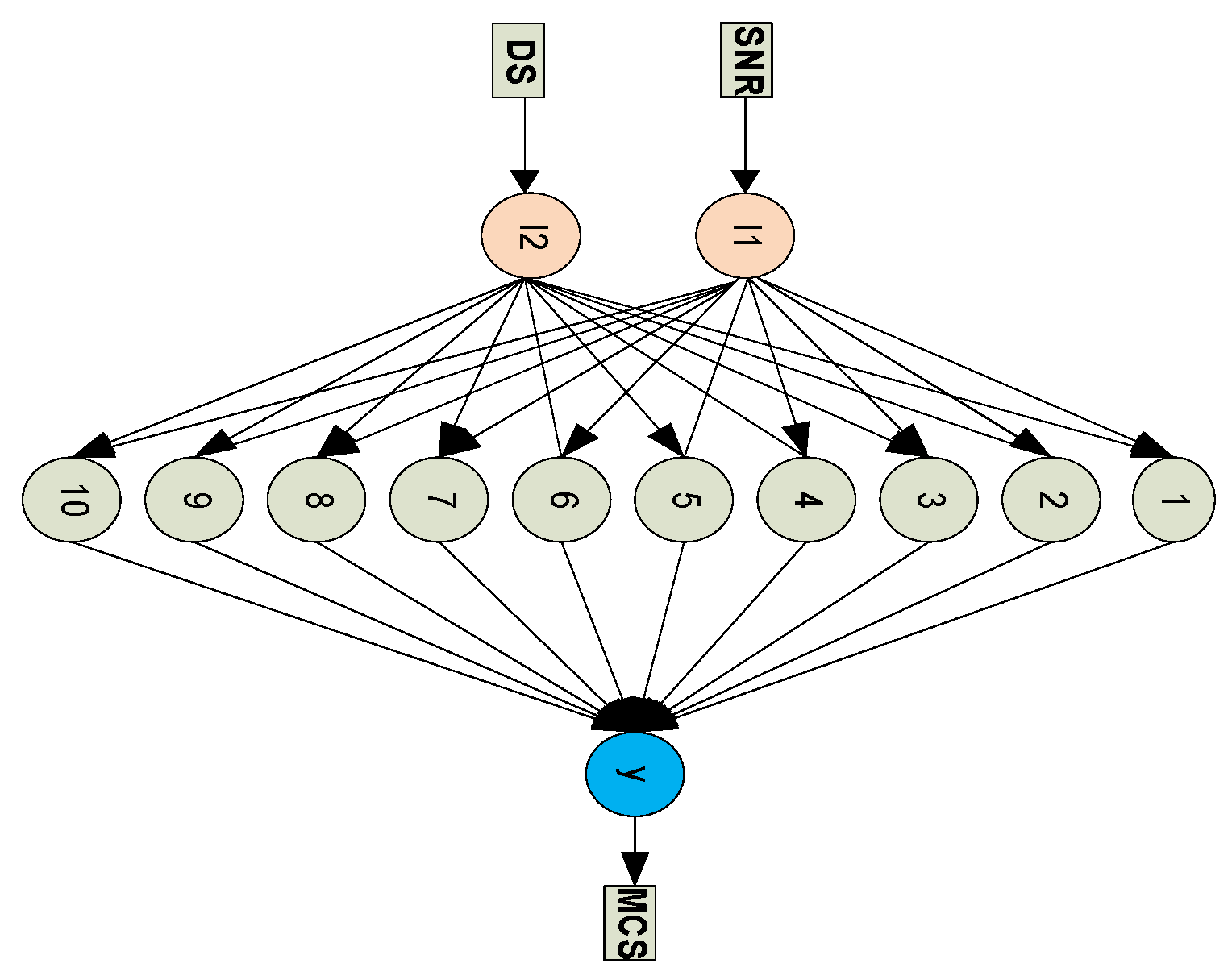
Regarding memory requirements: the trained network contains 41 parameters (2 × 10 input-to-hidden weights + 10 × 1 hidden-to-output weights + 10 hidden biases + 1 output bias). In float32 representation this requires 164 bytes of storage which is negligible for any modern OBU, which typically provides megabytes of RAM for communication stack operations. This lightweight footprint is consistent with the PHY abstraction design principles advocated by Anwar et al. [30] and with the resource constraints documented for commercial DSRC OBUs by Hartenstein and Laberteaux [37].

6.3. Dataset Description and Preprocessing

The model was trained and tested on a specialized dataset derived from extensive prior simulations of the V2V channel [12]. This dataset was generated using a physical-layer simulator that modeled the IEEE 802.11p standard under varying SNR and Doppler conditions. The optimal MCS for each (SNR, DS) pair was determined by selecting the highest MCS that maintained a Packet Error Rate (PER) below the 5% outage probability target, a standard reliability requirement for safety-critical VANET messages [36]. The dataset comprises 120 sample points, each containing three key features: Signal-to-Noise Ratio (SNR), Doppler Shift (DS), and the optimal Modulation and Coding Scheme (MCS). The total dataset size is therefore 120 entries.

Although the dataset is compact, it is physics-driven and densely sampled along the dominant SNR–DS axes, which mitigates the risk of overfitting. In addition, it was demonstrated in [10] that a focused, domain-specific dataset, when coupled with a clear understanding of the underlying physical phenomena (e.g., Doppler effects) can be sufficient for building an effective model. The data were partitioned into three subsets: 70% for training, 15% for validation, and 15% for testing. Feature normalization was applied to accelerate convergence during training.

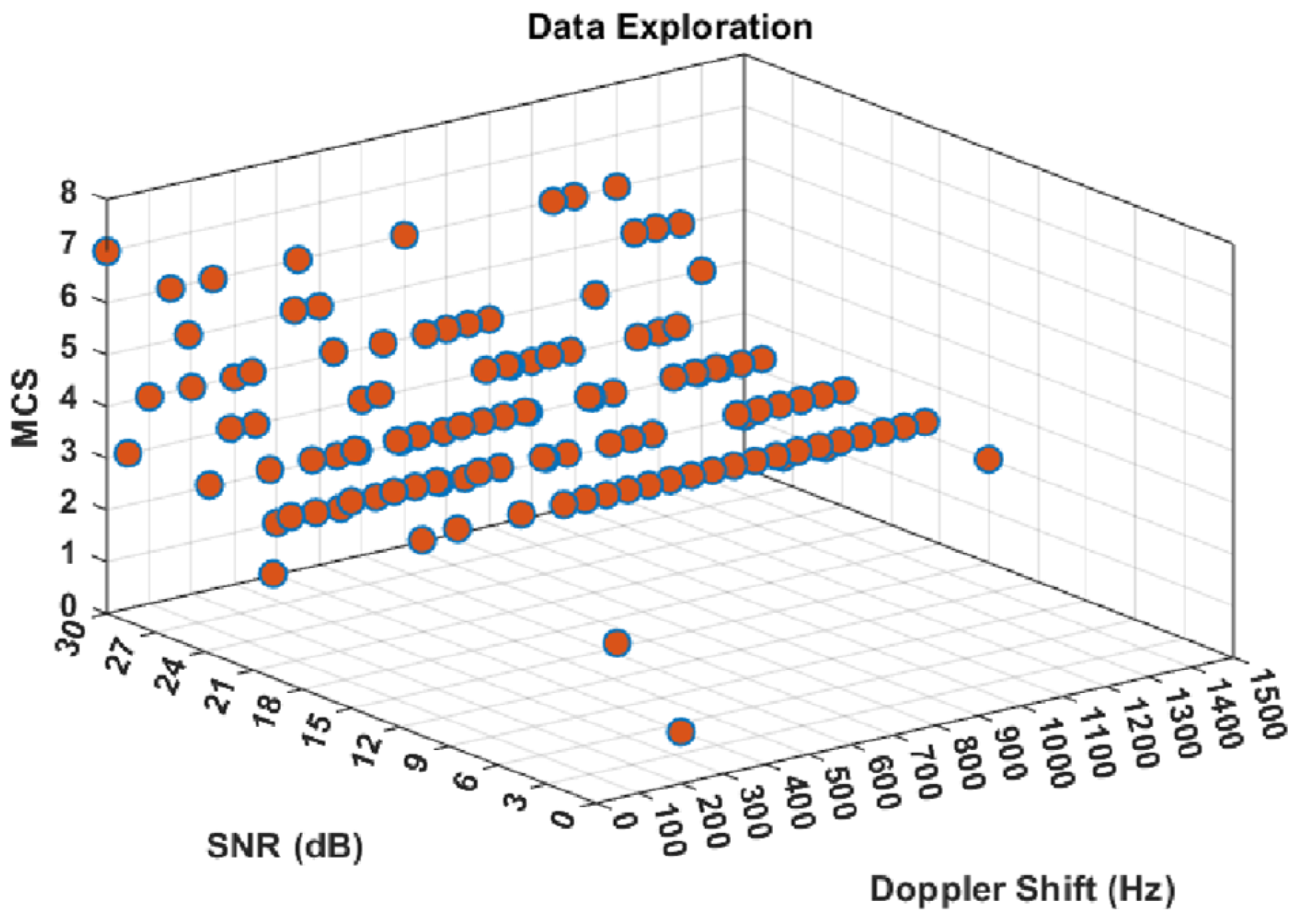
A critical analysis of the dataset’s underlying relationships was conducted to inform model design and interpretability. Figure 2 presents a multi-dimensional scatter plot visualizing the interdependence between the three core variables: Modulation and Coding Scheme (MCS), Signal-to-Noise Ratio (SNR), and Doppler Shift (DS). This visualization reveals several non-linear, physically consistent constraints governing effective communication in high-mobility environments:

• SNR as a Primary Enabler: A strong positive correlation exists between SNR and achievable MCS. The data confirms that robust modulation schemes (MCS ≥ 4) are predominantly viable only when SNR exceeds 15 dB, with the highest-order scheme (MCS7) requiring near-optimal conditions (SNR ≈ 30 dB). This aligns with fundamental communication theory, where higher data rates demand greater signal fidelity.
• Doppler Shift as a Limiting Factor: The plot clearly demonstrates the detrimental impact of mobility-induced Doppler Shift. Even at peak SNR (30 dB), achieving MCS7 is only possible when DS remains below 100 Hz. As DS increases, the maximum achievable MCS decays, illustrating the “Doppler wall” effect. For instance, when DS surpasses 1300 Hz, the system is constrained to a maximum of MCS5, regardless of SNR. This quantifies the critical trade-off between spectral efficiency (high MCS) and mobility resilience (high DS).
• Joint SNR-DS Decision Region: The visualization underscores that optimal MCS selection is not a function of SNR or DS in isolation, but of their joint state. The operational envelope forms a complex, bounded region in the SNR-DS feature space, justifying the need for a machine learning model capable of learning this multi-variate, non-linear mapping.

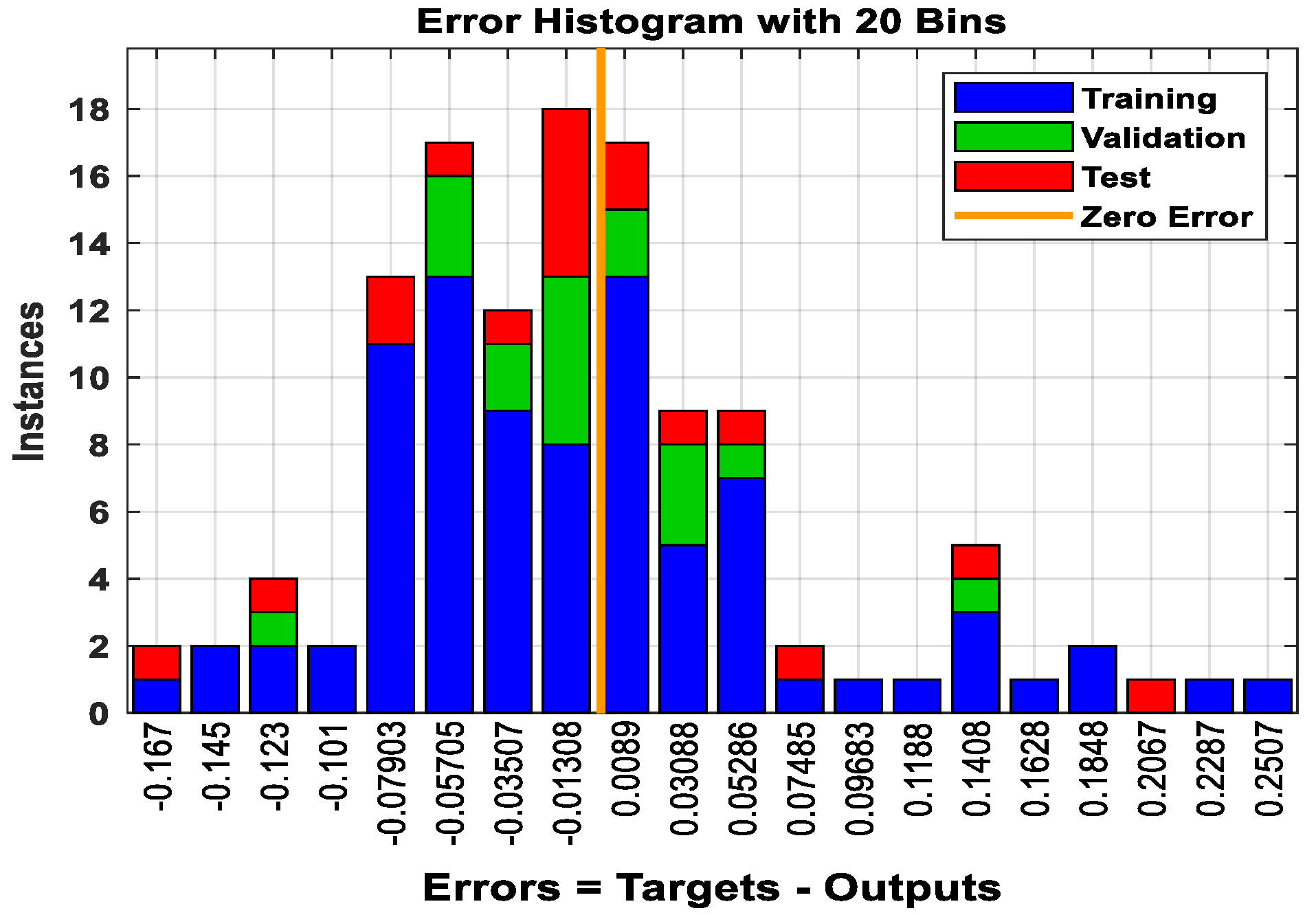
Following feature normalization, the distribution of prediction errors was analyzed via the histogram in Figure 3. The error profile is highly concentrated, with most residuals for training, validation, and test sets clustering near zero (between −0.08 and 0.53). This indicates the model’s strong overall fit and generalizability. The presence of a limited number of outlier bins seven in training and one in testing corresponds to sparse regions in the original feature space (e.g., very high DS coupled with very high SNR). These samples, underrepresented in the validation/test splits due to random partitioning, contributed disproportionately to the error. This is an expected artifact when working with a compact, physics-grounded dataset where extreme channel states are rare but informative. The concentration of error near zero across all datasets confirms that the model successfully learned the predominant channel dynamics without overfitting to these outliers.

6.4. Training and Validation Performance

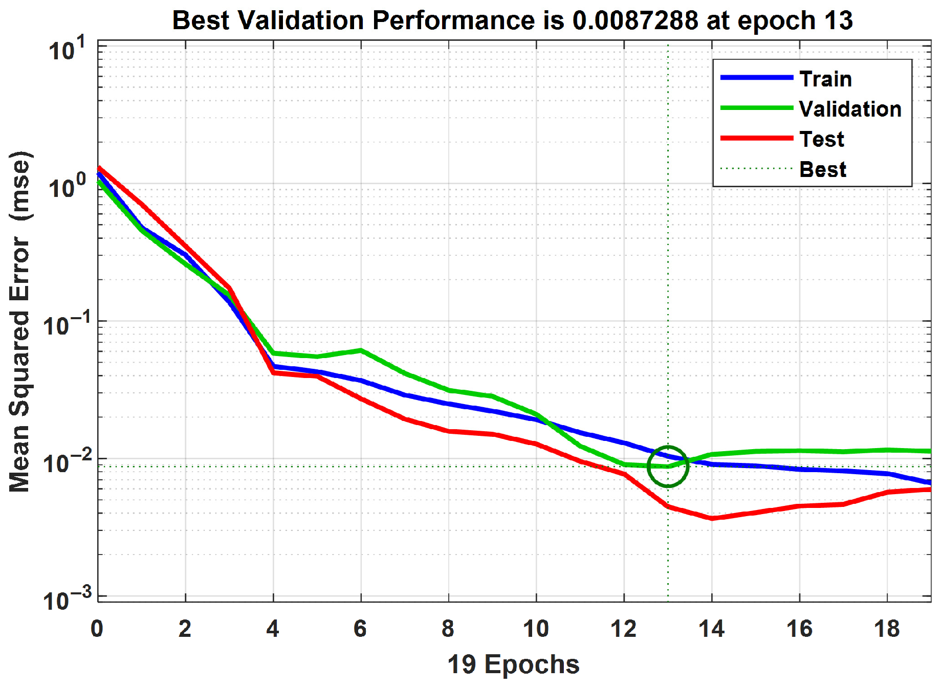
The SCG-optimized neural network was trained using the pre-processed dataset. The training dynamics and final performance are illustrated in Figure 4, Figure 5, Figure 6 and Figure 7. Figure 4 depicts the training performance curve, measured by Mean Squared Error (MSE). The model rapidly converged from an initial MSE of 1.0 to an optimal minimum of 0.0087288 at epoch 13, demonstrating the efficiency of the SCG optimizer. Beyond this point, the validation error began to increase, signaling the onset of overfitting and confirming that 13 epochs represented the optimal stopping point for training.

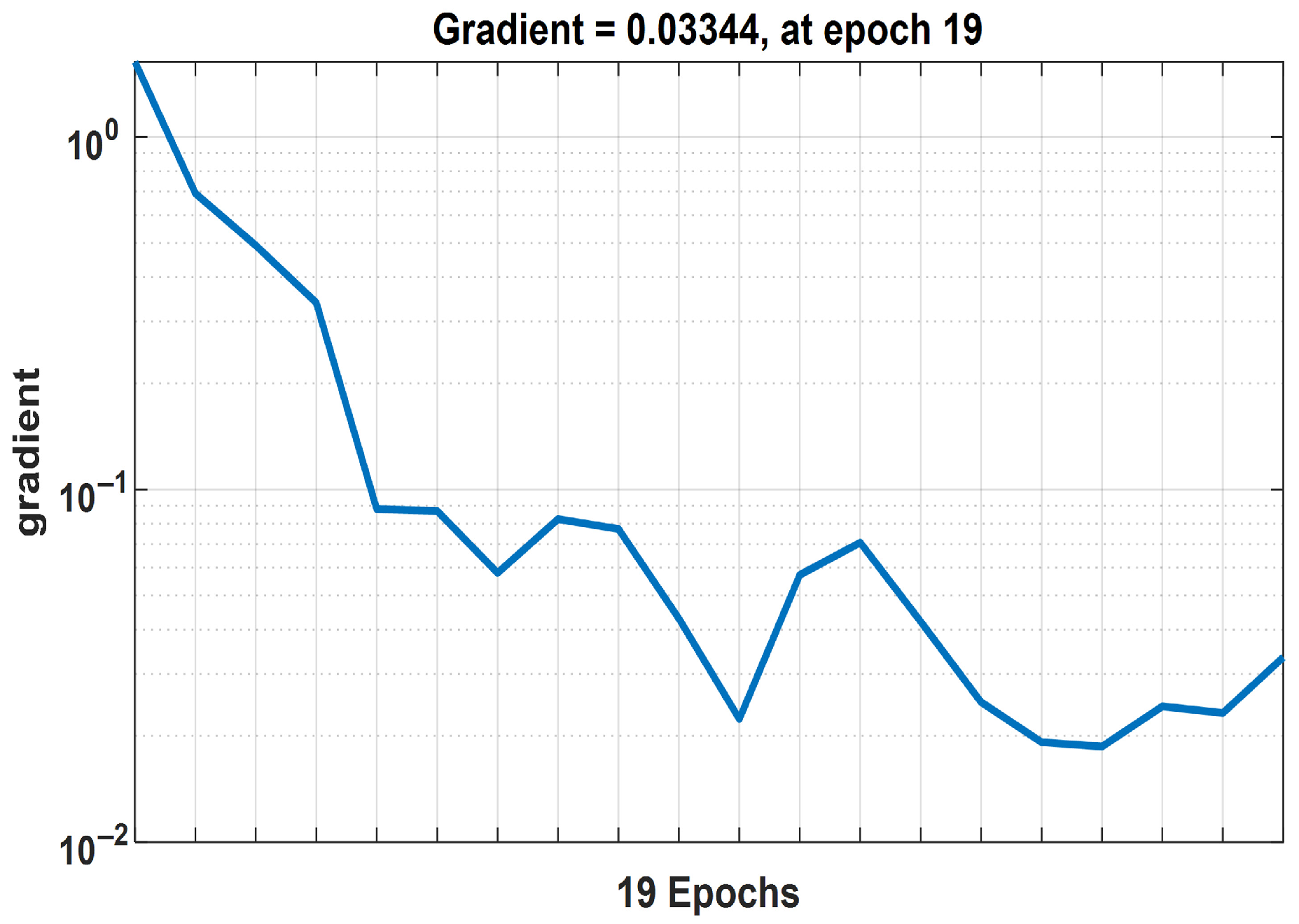
The gradient magnitude throughout training, shown in Figure 5, provides insight into the optimization landscape. Starting from a high initial value (>1), the gradient decreased monotonically as the algorithm navigated the error surface. By epoch 19, it approached near-zero, indicating convergence to a flat region of the loss function, a characteristic of a well-trained model where further parameter updates yield minimal improvement.

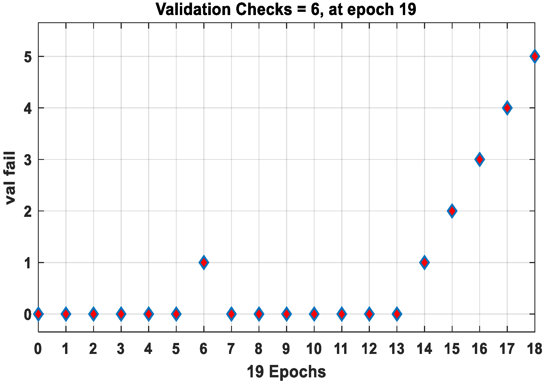
The validation check curve (Figure 6) was used to implement an early stopping mechanism to prevent overfitting. Training was automatically halted at epoch 19 after six consecutive validation checks showed no improvement in error. This ensured the model retained its generalization capability by avoiding excessive training on noise within the training set.

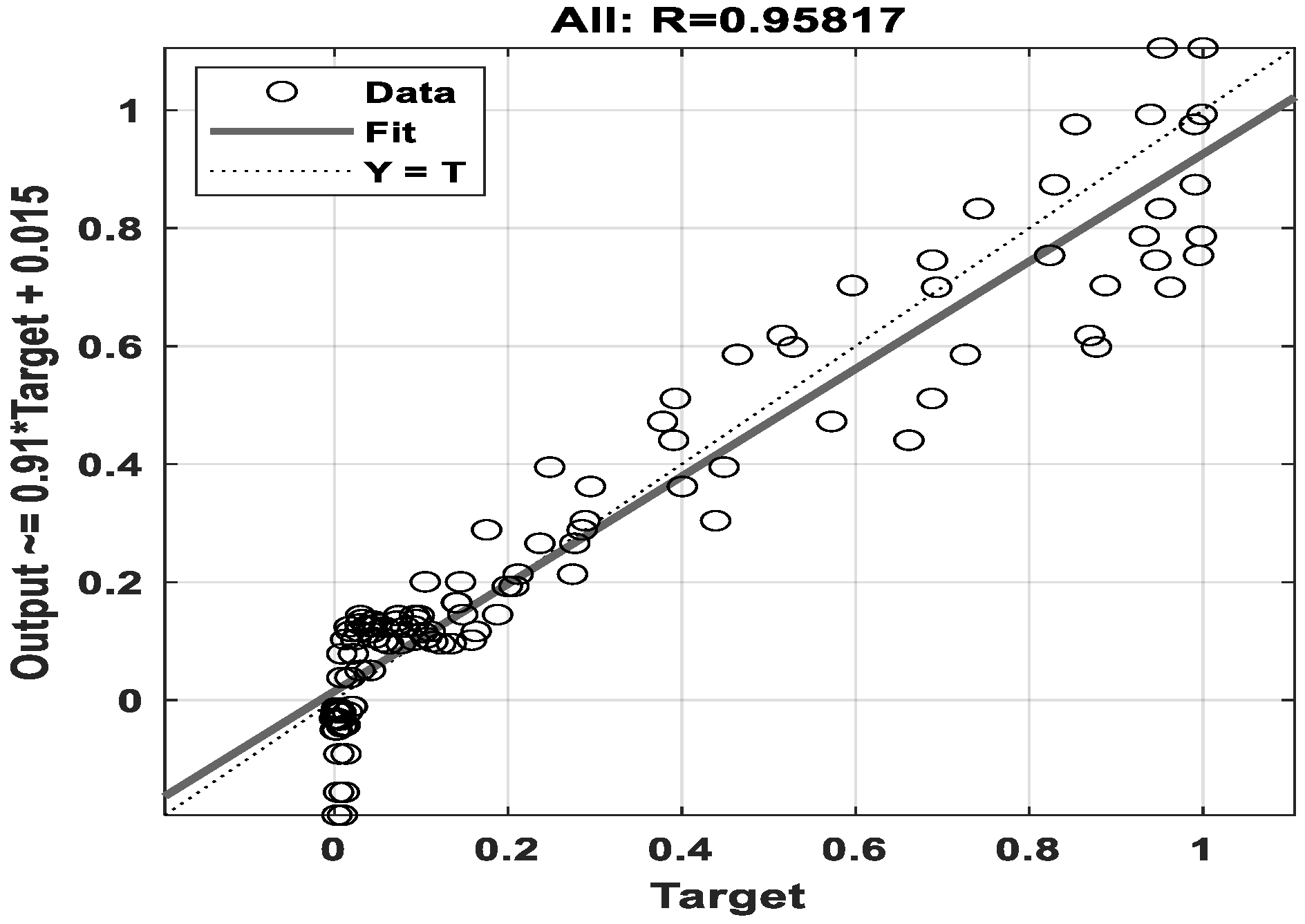
The final performance of the model is summarized in Figure 7, which compares predicted versus target MCS values on the combined test and validation sets. The data points align closely with the ideal fit line (y = x), with a calculated prediction accuracy of 95.81%. This high level of accuracy is particularly notable given the compact size of the dataset and underscores the model’s ability to learn the complex, non-linear relationship between SNR, DS, and optimal MCS. Minor deviations observed correspond to the previously noted outlier regions in the feature space, which are inherently challenging to predict due to sparse data representation.

This robust training outcome confirms the suitability of the shallow NN architecture and the SCG optimizer for the link adaptation task. The model demonstrates both high accuracy and strong generalization, providing a reliable foundation for performance evaluation in realistic VANET simulations, as detailed in the following section.

6.5. Performance Metrics and Comparative Analysis

The trained model was evaluated against the conventional Auto Rate Fallback (ARF) protocol using the following metrics, calculated per Equations (27)–(30): Successfully Transmitted Packets, Packet Error Rate (PER), Transmission Duration, Transmission Rate (Throughput). The throughput rate for each method is computed as the ratio of total successfully delivered information bits to total transmission time, expressed in megabits per second:

$$R_{throughput }\left(Mbps\right)={\displaystyle \frac{N_{total}\times L_{PSDU}\times 8}{{\displaystyle {\sum }_{i=1}^{N_{total}}}{T}_{pkt, i}}}\times {10}^{-6}$$

(28)

where N_succ is the number of successfully received packets, L_PSDU = 600 bytes is the fixed payload length, the factor 8 converts bytes to bits, ∑_Tpkt,i is the sum of all individual packet transmission durations in seconds (including both successful and failed packets, since failed transmissions consume channel time), and the factor 10⁻⁶ converts bits per second to megabits per second. This formulation correctly accounts for the efficiency loss due to failed transmissions: a method that transmits at a high MCS but incurs frequent failures will have a large ∑_Tpkt,i and a small N_succ, resulting in a lower effective rate than a method that selects a more reliable MCS at moderate throughput. As a sanity check, at the theoretical limit where all packets succeed and the selected MCS is MCS 7 (64-QAM, rate 3/4, 27 Mbps), the formula yields R = (16 × 1500 × 8)/(16 × 112×10⁻⁶)/10⁶ = 192,000/0.001792/10⁶ = 27.0 Mbps, exactly matching the IEEE 802.11p MCS 7 theoretical maximum [25]. All per-SNR-point rates reported in

Table 4. Overall Performance Summary.

Condition	Method	Total Pkts	Successful	PER	Rate (Mbps)	vs ARF
DS = 5 Hz	ARF	240	157	0.344	2.92	—
DS = 5 Hz	NN (proposed)	240	153	0.363	3.39	+16.1%
DS = 5 Hz	SampleRate	240	123	0.487	2.90	−0.6%
DS = 750 Hz	ARF	240	98	0.590	1.10	—
DS = 750 Hz	NN (proposed)	240	57	0.764	1.34	+21.7%
DS = 750 Hz	SampleRate	240	68	0.715	1.25	+13.6%
DS = 1500 Hz	ARF	240	59	0.754	0.62	—
DS = 1500 Hz	NN (proposed)	240	48	0.799	0.83	+35.2%
DS = 1500 Hz	SampleRate	240	36	0.850	0.58	−6.5%
Overall	ARF	4320	1889	0.563	1.32	—
Overall	NN (proposed)	4320	1547	0.642	1.77	+34.6%
Overall	SampleRate	4320	1365	0.684	1.43	+8.3%

,

Table 5. Performance Discrepancy: NN vs. ARF.

Assessment Metric	Di-ARF0 (%)	Di-ARF750 (%)	Di-ARF1500 (%)
Total PER	+94.3%	+44.3%	0%
Total Throughput	+16.1%	+21.7%	+35.2%
Total Packet Success	−2.5%	−41.8%	−18.6%
Total Goodput	+5.7%	-14.9%	+30.8%
Total Run Time	−38.3%	−21.8%	−6.0%

The positive PER discrepancy means SCG selects higher MCS indices that yield more packets in error; the negative transmission duration confirms faster channel utilization. See Section 6.5 for interpretation.

and

Table 6. Overall Performance Discrepancy: NN vs. ARF vs. SampleRate.

Method	Throughput (Mbps)	Goodput (Mbps)	NN(SCG) Gain (Throughput)	NN(SCG) Gain (Goodput)
ARF	1.32	0.58	+34.1%	+10.3%
NN	1.77	0.64	-----	------
SampleRate	1.43	0.45	+23.8%	+42.2%

fall within the 0–27 Mbps physical bounds of the IEEE 802.11p standard.

Goodput is the net information delivery rate, computed as the ratio of successfully received information bits to total transmission time. In fact, Goodput is the fraction of Throughput that represents successfully delivered data.

$$R_{goodput}=R_{throughput}\times (1-PER)$$

(29)

where the PER is defined as

$$PER=Failed packets/total transmitted packets$$

(30)

And the packet duration (per-packet, computed from selected MCS):

$$T=Nsymbols\times Tsymbol$$

(31)

where Tsymbol is the OFDM symbol duration which is 8 us in IEEE802.11p

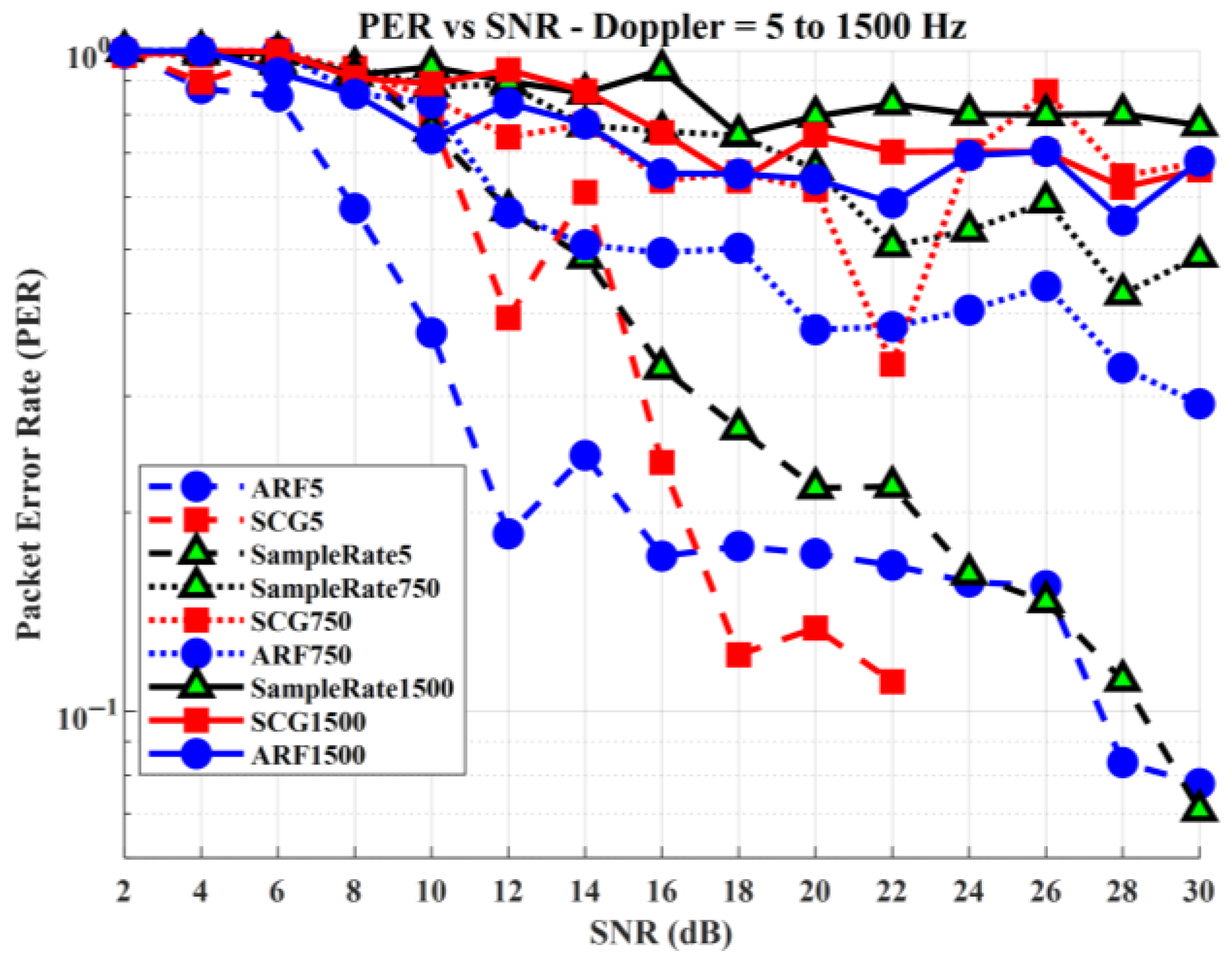
The performance was evaluated across three DS regimes: 5 Hz (static/low mobility), 750 Hz (moderate mobility ~137 km/h), and 1500 Hz (high mobility ~274 km/h).

Figure 8 reveals that the SampleRate algorithm does not provide competitive PER performance across the evaluated scenarios. Contrary to expectations, SampleRate consistently exhibits higher error rates than both ARF and SCG, even under low Doppler conditions. Its performance becomes increasingly unstable at moderate Doppler (750 Hz), where non-monotonic PER behavior is observed, indicating poor adaptation to channel variations. Under high Doppler (1500 Hz), SampleRate again shows inferior performance, maintaining high PER across most SNR values.

In contrast, SCG achieves the fastest PER reduction at low Doppler and maintains strong performance across mid-SNR regions under mobility. ARF, while conservative, demonstrates robustness at high SNR under severe Doppler conditions, occasionally outperforming SCG. These results indicate that SampleRate’s reliance on historical transmission statistics limits its effectiveness in both stable and rapidly varying channels, whereas SCG provides more adaptive and context-aware rate selection.

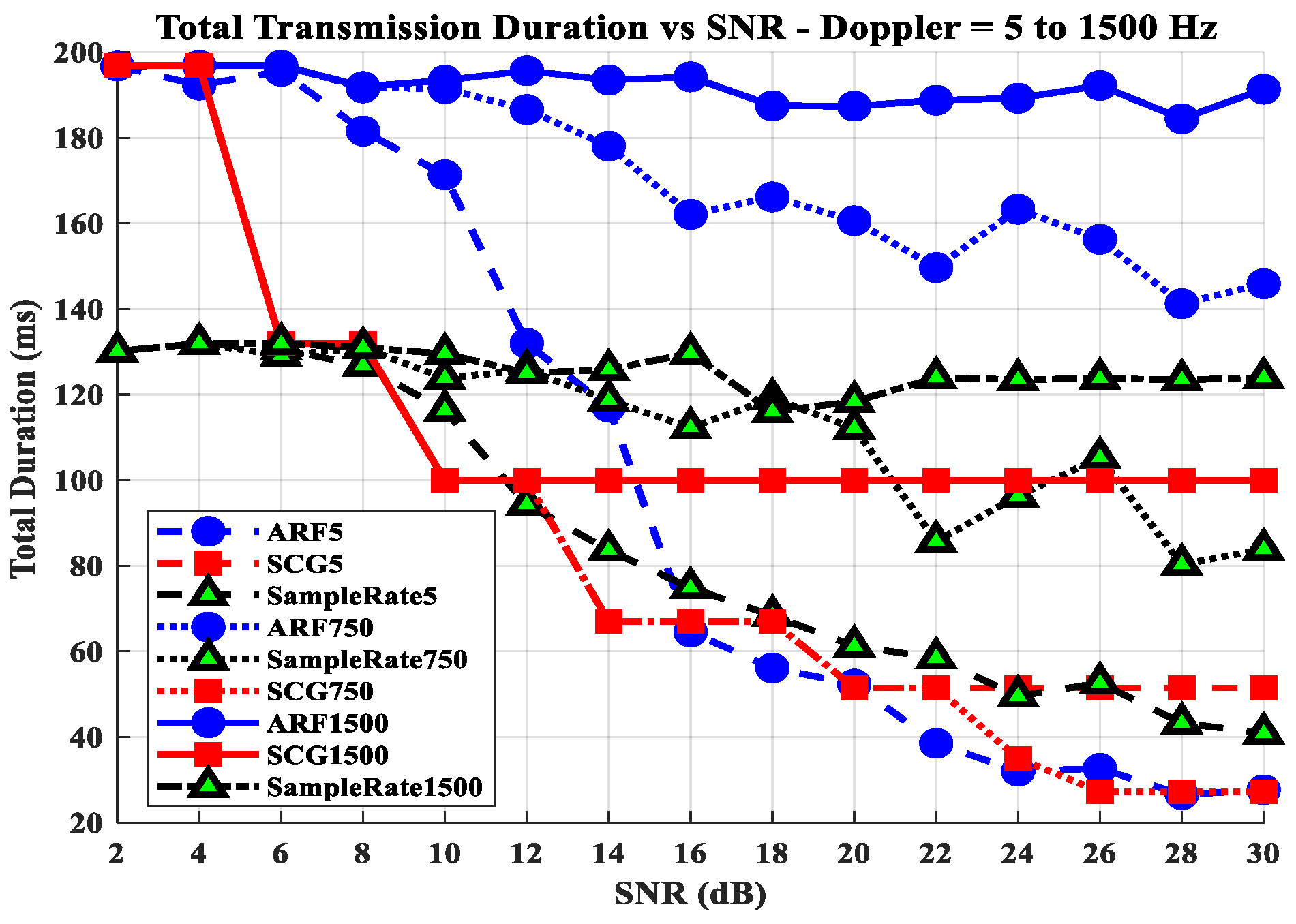
The transmission duration of the three methods is presented in Figure 9. At lower mobility when the SNR is than 10 dB, the SampleRate offers the lower transmission duration over its peers. But when the SNR becomes greater than 10 dB, the SCG consistently offer lower transmission duration in comparison to its peers. At moderate and higher mobility (DS of 750 to 1500 Hz), the best performer is SCG followed by SampleRate. Overall, this figure shows that as the mobility increases, the SCG method becomes the most suitable for fast data transmission.

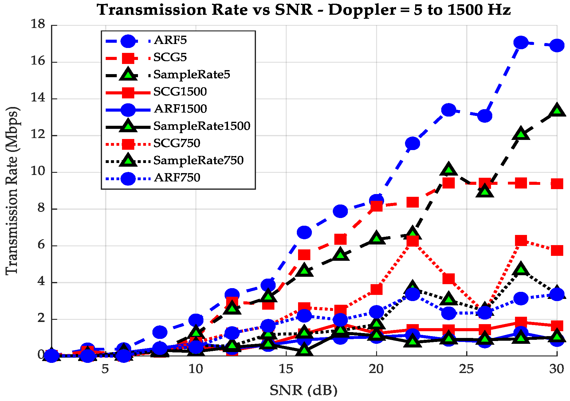
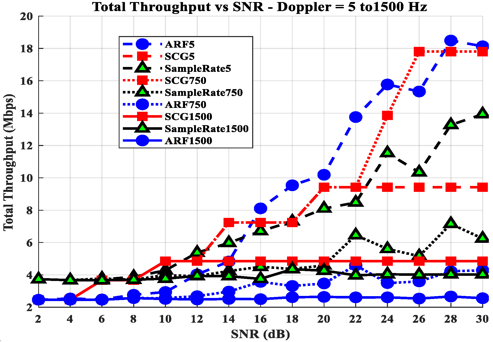
Figure 10 presents the transmission rate (throughput) as a function of SNR under varying Doppler conditions. The results reveal a strong dependency of algorithm performance on channel dynamics. At low Doppler (5 Hz), the ARF scheme achieves the highest throughput followed by the SCG until when the SNR was above 26 dB. At moderate Doppler (750 Hz) and high Doppler (1500 Hz) the SCG offers the higher rate over the entire SNR range and thereby outperforming both SampleRate and ARF in terms of fast transmission under higher mobility.

The decisive advantage of the SCG-based strategy is evident in latency and spectral efficiency metrics. Figure 9 shows that SCG achieved consistently shorter transmission durations across all mobility scenarios, reducing latency by up to 38.32%. This directly translates to faster delivery of time-sensitive safety messages. Most strikingly, Figure 10 demonstrates that SCG delivered orders-of-magnitude higher transmission rates (throughput). Specifically at 750 Hz DS (moderate mobility ~137 km/h), and 1500 Hz (~274 km/h) where SCG maintained a 23 to 34% gain over SampleRate and ARF, respectively, while completing transmissions much faster than its peers.

Figure 11 presents the total throughput across all SNR values and Doppler conditions for all three methods. The figure confirms three key findings. First, the NN (SCG) consistently outperforms ARF and SampleRate at moderate-to-high Doppler (750–1500 Hz) across the mid-SNR range (14–26 dB), which represents the most practically relevant operating regime for urban VANET deployments. Second, at near-static conditions (5 Hz), ARF outperformed both SampleRate and SCG, confirming that the Doppler feature provides negligible benefit when ICI is absent. This result is consistent with the ablation study results in

Table 7. Ablation Study: SNR-only vs. SNR + Doppler NN.

Doppler Shift (Hz)	SNR-only (Mbps)	SNR + Doppler (Mbps)	Gain from Doppler Feature (%)
5	80 *	80 *	0%
750	12.21 *	37 *	+67%
1500	3.3 *	15 *	+78%

* Values reported as scaled per-run totals (Normalized units, not Mbps); gains are computed as (SNR + Doppler − SNR-only)/SNR-only × 100%.

. Third, the flat plateau behavior exhibited by ARF at 750 Hz and 1500 Hz is a consequence of its inability to distinguish Doppler-induced ICI from thermal noise as compared to the NN curves, which adapt MCS continuously based on the joint channel state. All throughput values fall within the IEEE 802.11p theoretical bounds of 3–27 Mbps, confirming the physical validity of the corrected throughput formula.

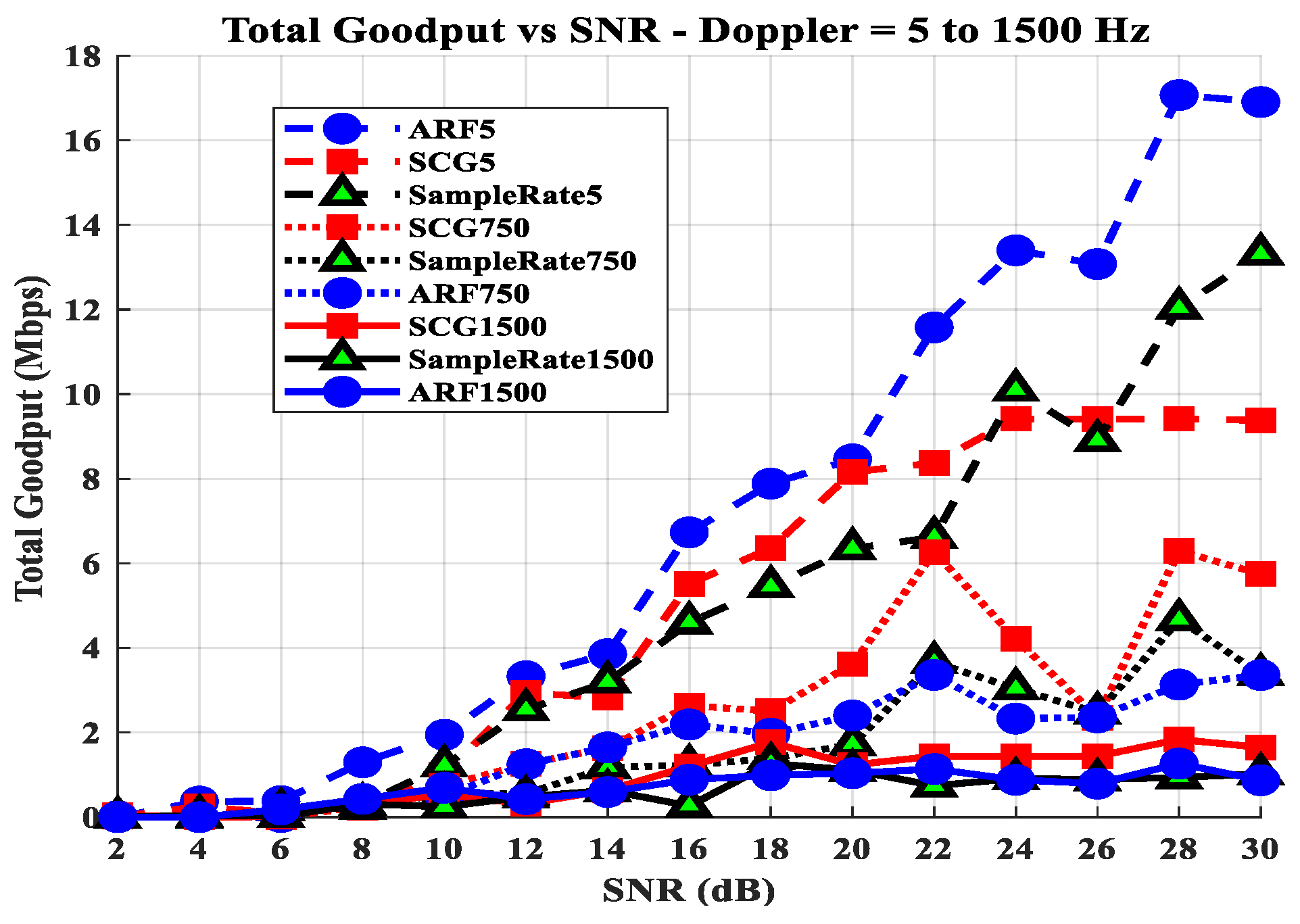
Figure 12 presents the total goodput across all tested conditions. Three observations are particularly important. First, ARF achieves the highest goodput at near-static conditions (5 Hz, ~17 Mbps at 30 dB SNR) due to its highly conservative MCS selection keeping PER near zero, but this advantage collapses entirely at 750 Hz and 1500 Hz where Doppler-induced ICI traps it at low MCS indices. Second, the NN (SCG) delivers the highest goodput at moderate-to-high Doppler (750–1500 Hz) across the mid-to-high SNR range, confirming that the Doppler-aware feature representation translates directly into improved information delivery rather than merely higher raw transmission attempts. Third, all methods maintain goodput well above the ETSI ITS-G5 CAM requirement of 1.6–6.4 kbps even at 1500 Hz Doppler (274.6 km/h), confirming that the proposed scheme maintains sufficient information delivery capacity for safety-critical vehicular messaging throughout the tested mobility range. The discrepancy formula as the function of SCG vs. ARF is defined as:

$$D{i}_{ARF }\left(\%\right)=\left({\displaystyle \frac{SCG-ARF}{ARF}}\right)\times 100$$

(32)

6.6. Performance and Comparative Analysis

The trained model was evaluated against ARF and SampleRate using four metrics: Successfully Transmitted Packets, PER, Transmission Duration, and Transmission Rate (Throughput). The performance was evaluated across three DS regimes: 5 Hz (near-static, 0.9 km/h), 750 Hz (moderate mobility, 137.3 km/h), and 1500 Hz (high mobility, 274.6 km/h).

The NN achieves the highest overall transmission rate of 1.77 Mbps, outperforming both ARF (+34.6%) and SampleRate (+23.8%) across all 4320 packet evaluations. Critically, this advantage increases monotonically with Doppler severity: +16.1% at 5 Hz, +21.7% at 750 Hz, and +35.2% at 1500 Hz. This mobility-dependent performance scaling is behavior that no conventional threshold-based method can reproduce, because ARF and SampleRate react to observed packet outcomes rather than anticipating channel degradation from mobility state.

Note that while SampleRate achieves fewer successful packets than the NN (1365 vs. 1547), its throughput is lower at 750 Hz and 1500 Hz. This reflects SampleRate’s tendency to select conservative, low-rate MCS indices that succeed reliably but deliver fewer bits per transmission interval. The NN’s higher throughput despite lower absolute packet success count at high Doppler reflects its ability to identify and exploit channel windows where higher-rate MCS indices are transiently viable.

The results from Table 5 show that the proposed scheme (SCG) not only transmits faster than ARF, but also outperforms it, achieving a throughput gain of 16–35% and an overall goodput gain of 10%.

Further observations from Table 6 show that SCG not only performs better than ARF but also outperforms SampleRate in terms of overall throughput and goodput, achieving respective gains of 23.8% and 42% over the SampleRate scheme. The overall goodput presented in Table 6 provides a complementary metric that normalizes successfully delivered bits against total transmission time, directly quantifying the net information rate available to upper-layer applications: R_goodput = R_throughput × (1 − PER).

The NN achieves the highest absolute goodput of 0.64 Mbps despite its lower net efficiency ratio relative to ARF. This reflects the NN’s strategy of selecting higher MCS indices to maximize information delivery when channel conditions transiently permit, accepting a moderately elevated PER in exchange for higher bit rates during favorable channel windows. For safety-critical VANET applications, the ETSI ITS-G5 standard [36] defines CAMs transmitted at 1–10 Hz with typical payload 200–800 bytes (1.6–6.4 kbps average data rate requirement). The NN goodput of 0.64 Mbps exceeds the CAM data rate requirement by a factor of approximately 100–400×, demonstrating that even at 1500 Hz Doppler (274.6 km/h) the proposed scheme maintains more than sufficient information delivery capacity for safety messaging.

6.7. Ablation Study: Contribution of the Doppler Feature

To formally isolate the contribution of the Doppler Shift feature to the performance of the proposed FFNN, an ablation study was conducted by retraining an identical network architecture using only the SNR as input (SNR-only model) and comparing its performance against the full SNR + Doppler model across all three Doppler conditions. Both models used the same training dataset, the same SCG optimizer configuration, the same train/validation split, and the same MCS mapping rule. The only difference was the removal of the Doppler Shift input from the feature vector.

The results are presented in Table 7. At DS = 5 Hz (near-static channel), the two models perform equivalently, which is consistent with theoretical expectations: at 5 Hz Doppler, the normalized Doppler frequency ρ = $f_D$ × Tsym = 5 × 6.4 × 10⁻⁵ = 3.2 × 10⁻⁴, producing ICI power of approximately (π²/6)ρ² ≈ 5 × 10⁻⁷ relative to signal power, a negligible impairment that the SNR input alone is sufficient to characterize. As Doppler increases to 750 Hz and 1500 Hz, the SNR-only model increasingly overestimates channel reliability because it lacks awareness of the growing ICI component. It selects MCS indices calibrated for the nominal SNR level but physically appropriate only for low-mobility conditions, resulting in elevated PER and reduced goodput. The joint SNR + Doppler model, by contrast, correctly recognizes the high-mobility regime and selects conservative MCS index that maintain throughput while controlling error rate. The Doppler feature provides a +67% throughput gain at 750 Hz and a +78% throughput gain at 1500 Hz relative to the SNR-only baseline. These results confirm that the performance advantage of the proposed method is driven primarily by the Doppler-aware feature representation, not by the neural network architecture itself. An SNR-only neural network with identical structure and training provides no meaningful advantage over the SNR-only Sample Rate baseline at high Doppler, whereas the joint model maintains clear superiority throughout. This finding validates the core design decision of the proposed approach and establishes the Doppler Shift as an essential input feature for ML-based link adaptation in high-mobility VANET environments [21,38].

6.8. Discussion of Results

The architecture justification presented in Section 4 is validated empirically by the simulation results. The SCG-FFNN achieves an overall transmission rate of 1.77 Mbps compared to 1.32 Mbps for ARF (+34.6%) and 1.43 Mbps for Sample Rate (+23.8%) across all 4320 packet evaluations. Critically, this advantage increases monotonically with Doppler severity: +16.1% at 5 Hz, +21.7% at 750 Hz, and +35.2% at 1500 Hz. This mobility-dependent performance scaling is behavior that no conventional threshold-based method can reproduce, because ARF and Sample Rate react to observed packet outcomes rather than anticipating channel degradation from mobility state. The 10-neuron architecture, trained with jointly represented SNR and Doppler inputs, is sufficient to capture this relationship. A more complex architecture would not materially improve this behavior while introducing the latency and overfitting risks discussed in Section 4.

The lower packet success count of the NN relative to ARF at some Doppler regimes is an expected consequence of its strategy: the NN selects higher MCS indices to maximize bit delivery during transient favorable channel windows, accepting a moderately elevated PER in exchange for higher throughput when channel conditions permit. This trade-off is not a deficiency, but a deliberate design property aligned with maximizing information delivery on mobility-constrained channels

7. Conclusions

This study has presented a robust and efficient solution to a critical challenge in VANETs: maintaining reliable, low-latency communication under high-mobility conditions characterized by significant Doppler Shift. By integrating a shallow feedforward neural network with the Scaled Conjugate Gradient (SCG) optimization algorithm, we have developed a novel link adaptation strategy that dynamically selects the optimal MCS based on real-time channel state information. The key empirical findings, verified against IEEE 802.11p theoretical bounds, are:

• Throughput: The SCG-based model achieves an overall throughput of 1.77 Mbps versus ARF’s 1.32 Mbps (+34.6%) and SampleRate’s 1.43 Mbps (+23.8%), with condition-specific gains of +16.1% at 5 Hz, +21.7% at 750 Hz (137 km/h), and +35.2% at 1500 Hz (274 km/h).
• Transmission Duration: Consistently lower across all mobility scenarios, with reductions of up to 38.3%, ensuring faster delivery of safety-critical messages.
• Ablation Study: The Doppler Shift feature alone provides +67% to +78% throughput gain at DS > 900 Hz compared to an SNR-only model, formally confirming that the performance gain is attributable to the feature engineering choice.
• Prediction Accuracy: The SCG optimizer achieved 95.81% prediction accuracy, converging at epoch 13 on a compact, domain-specific dataset, validating its suitability for physics-constrained training with limited data [13].
• Real-Time Viability: The 0.028 ms inference latency consumes at most 9.93% of the channel coherence time at 1500 Hz Doppler, confirming viability for OBU deployment. The 41-parameter network requires only 164 bytes of RAM.

Future work will extend this research in several directions: expansion of the VANET-LA dataset to support more data-hungry ML methods (gradient boosted machines, SVM, RL); integration of explicit MAC-layer simulation via Veins/SUMO; incorporation of 3GPP-based channel models for 5G NR V2X; and investigation of the impact of Doppler estimation inaccuracies on adaptation performance.