Components for an Inexpensive CW-ODMR NV-Based Magnetometer


Abstract
1. Introduction
2. Materials and Methods
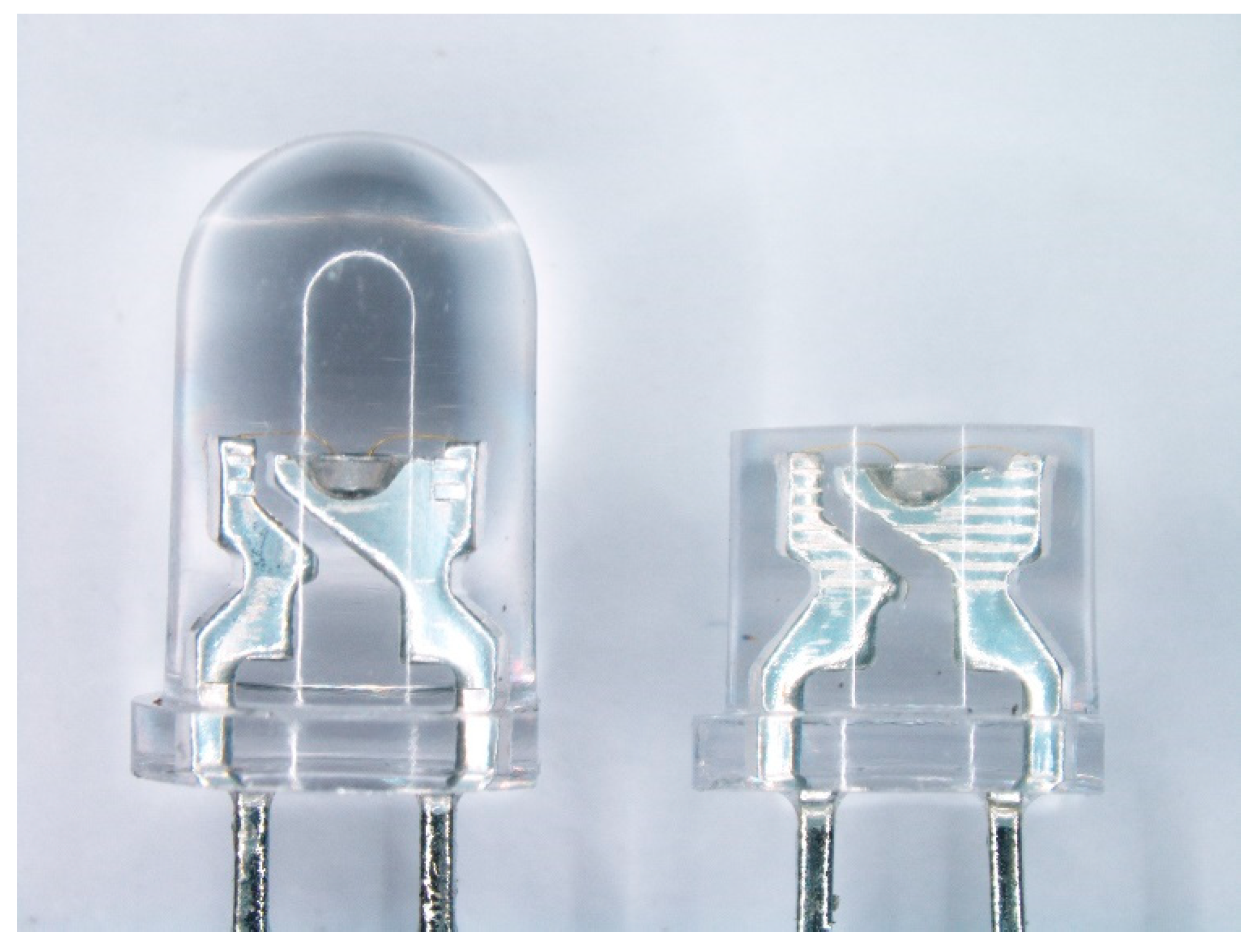
2.1. LED
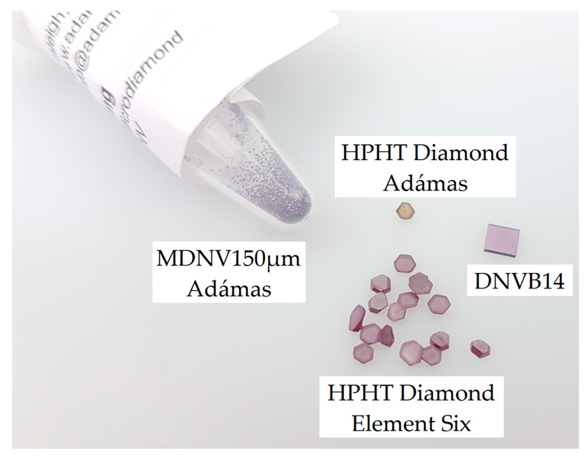
2.2. Diamonds
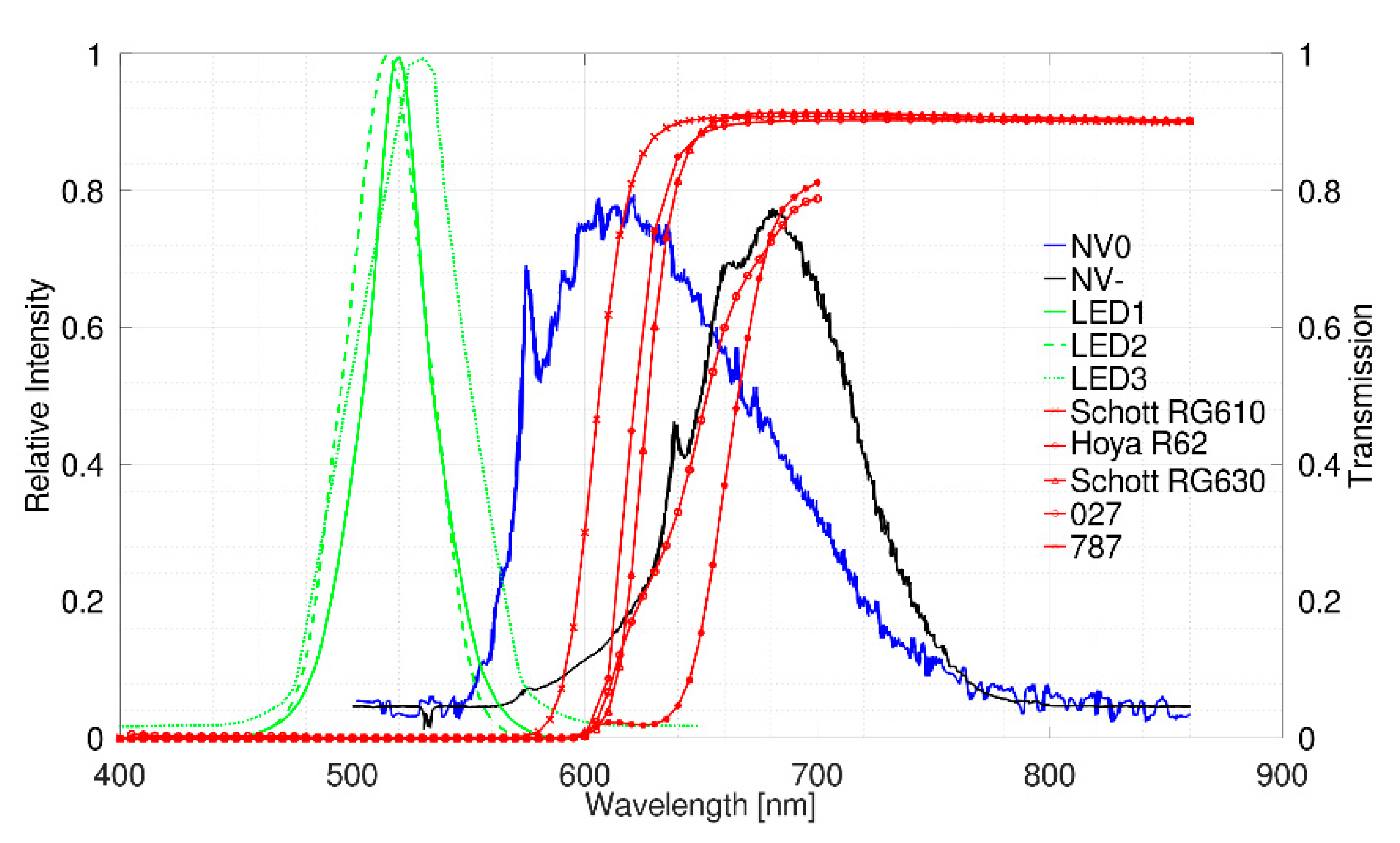
2.3. Color Filter
- LED as light source,
- LED as light source with various filters in front of it,
- LED as light source with a microdiamond attached to it and various filters
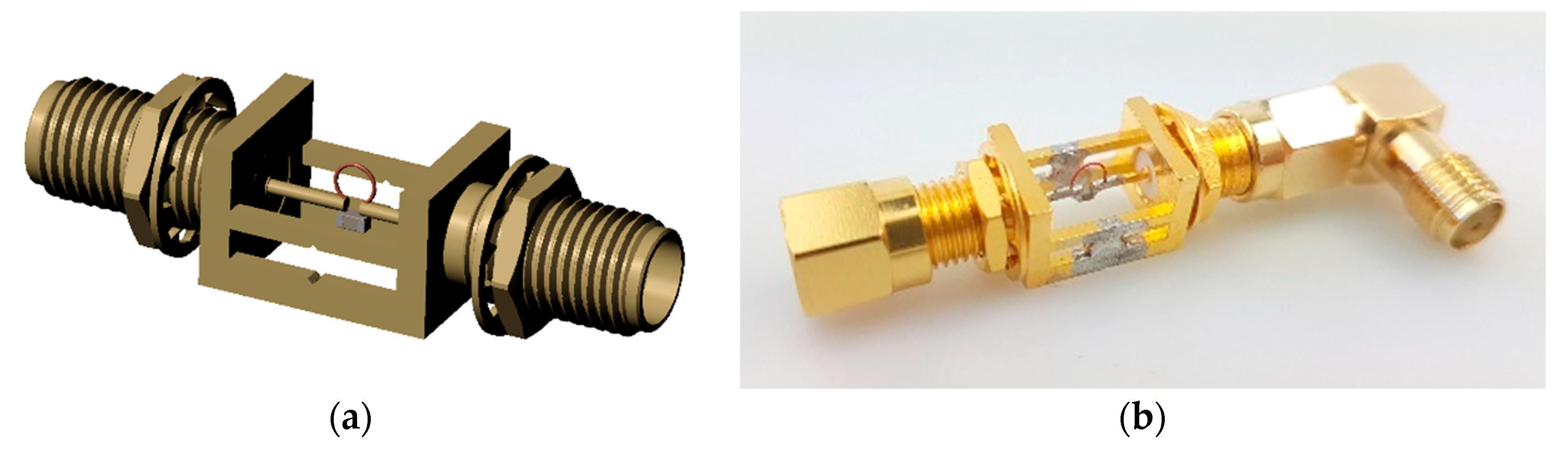
2.4. Resonator
2.5. Photodetector and TIA
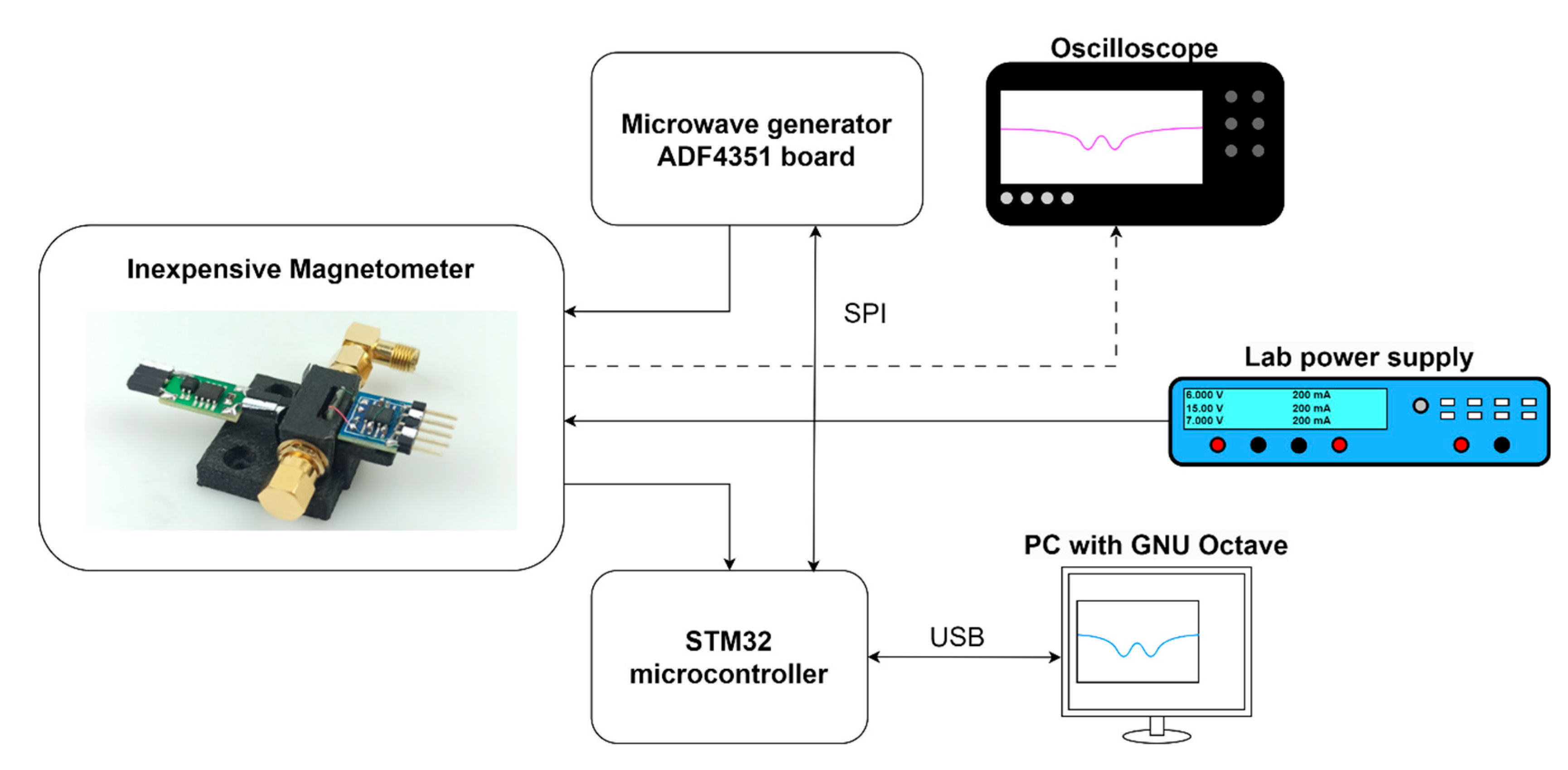
2.6. CW-ODMR Setup and Measurement
3. Results
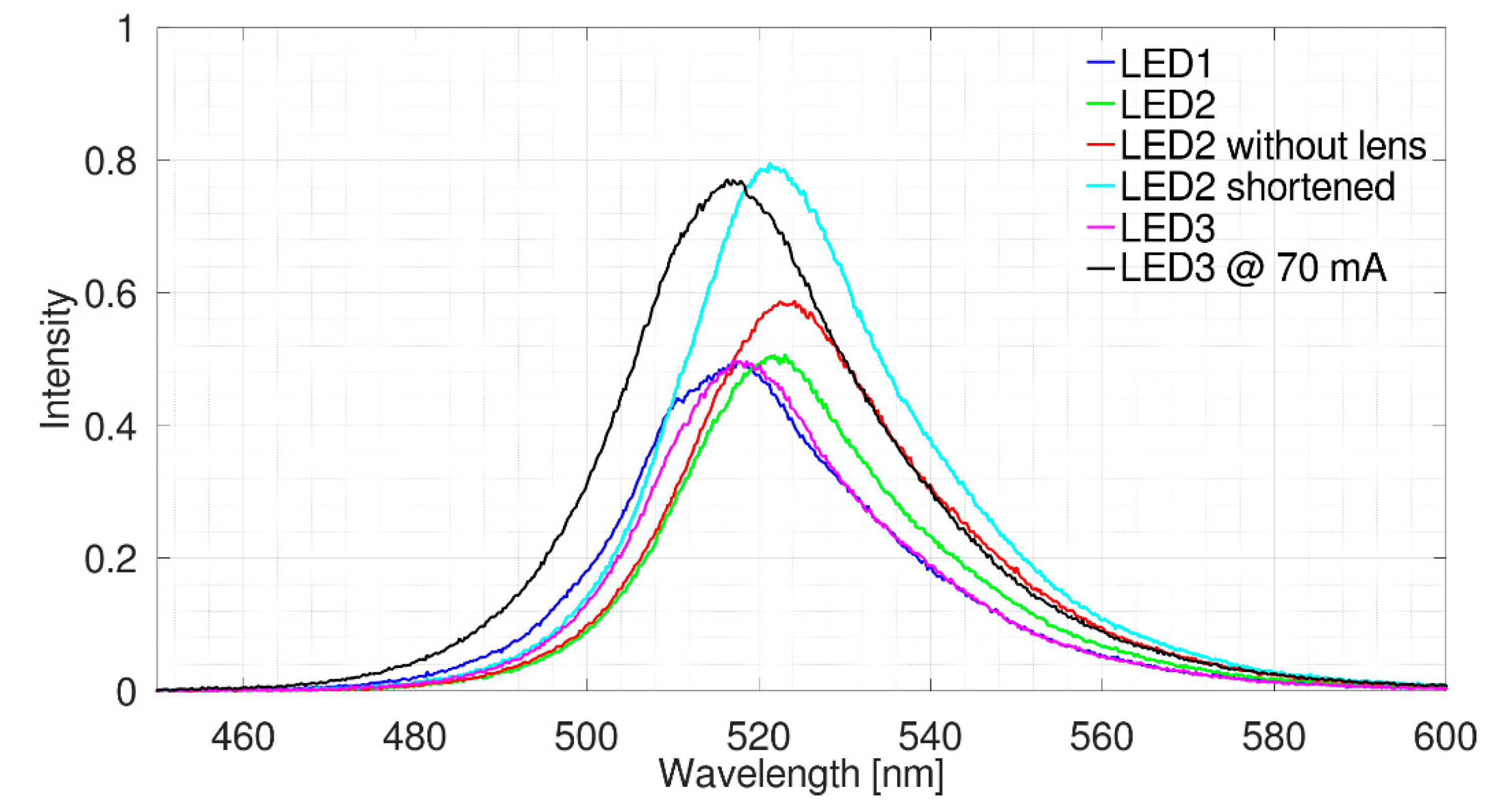
3.1. LEDs Measured with Spectrometer
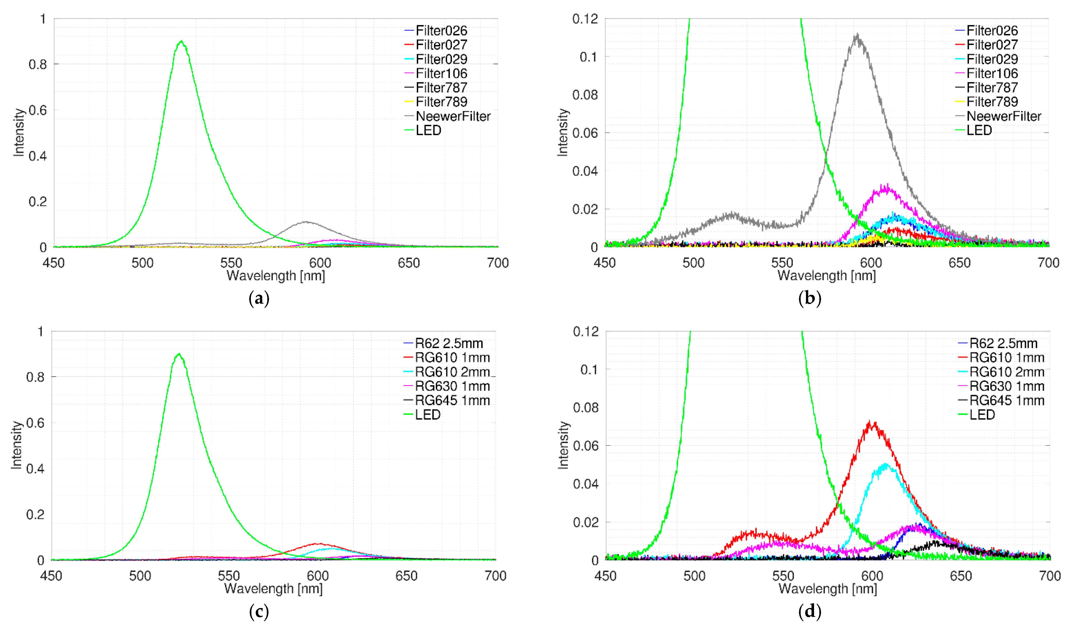
3.2. LED2 with Various Filters Measured with Spectrometer
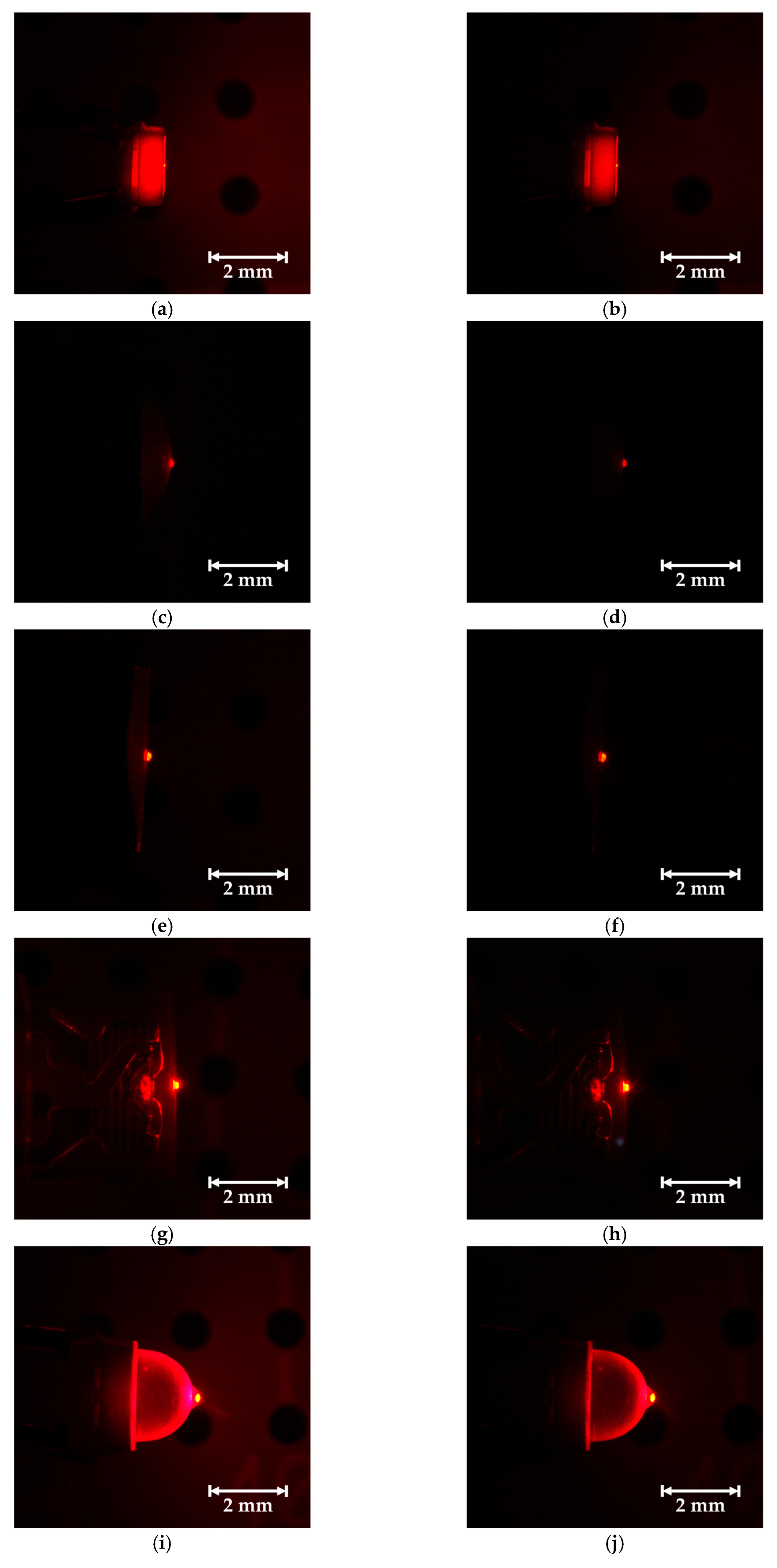
3.3. Microscope Images of LEDs with Microdiamond and Color Filters
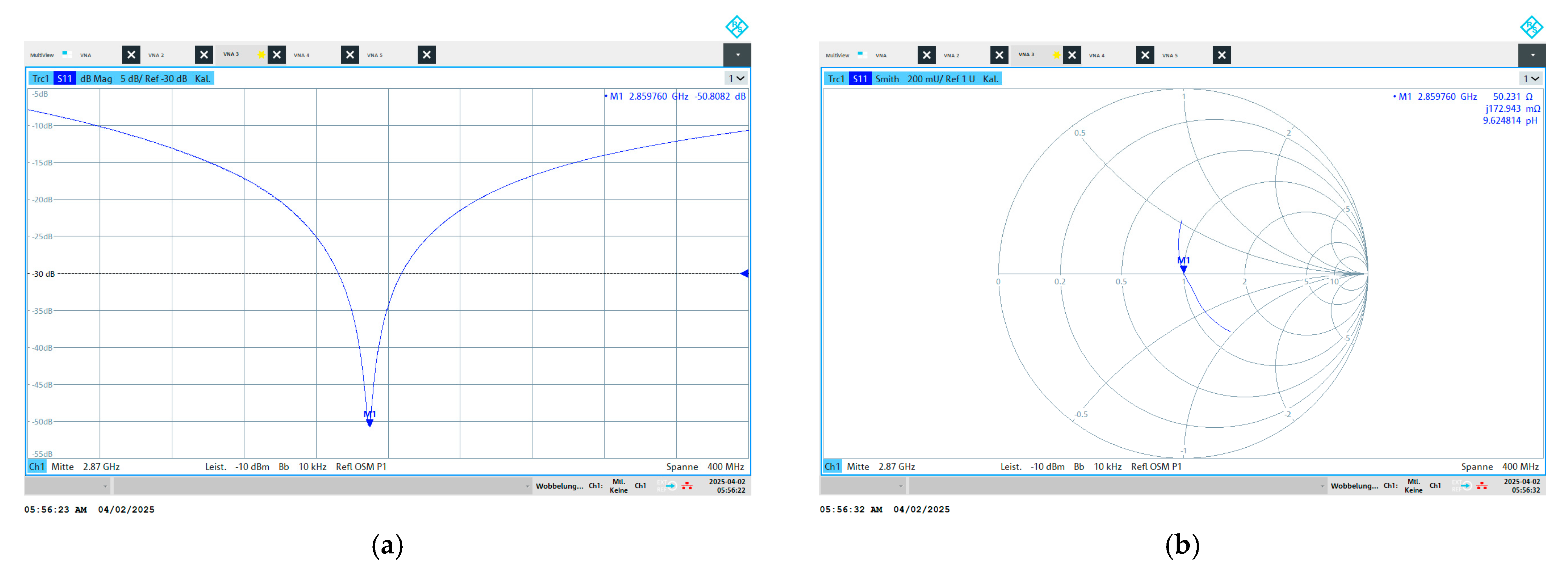
3.4. Resonator
3.5. Inexpensive Magnetometer Setup
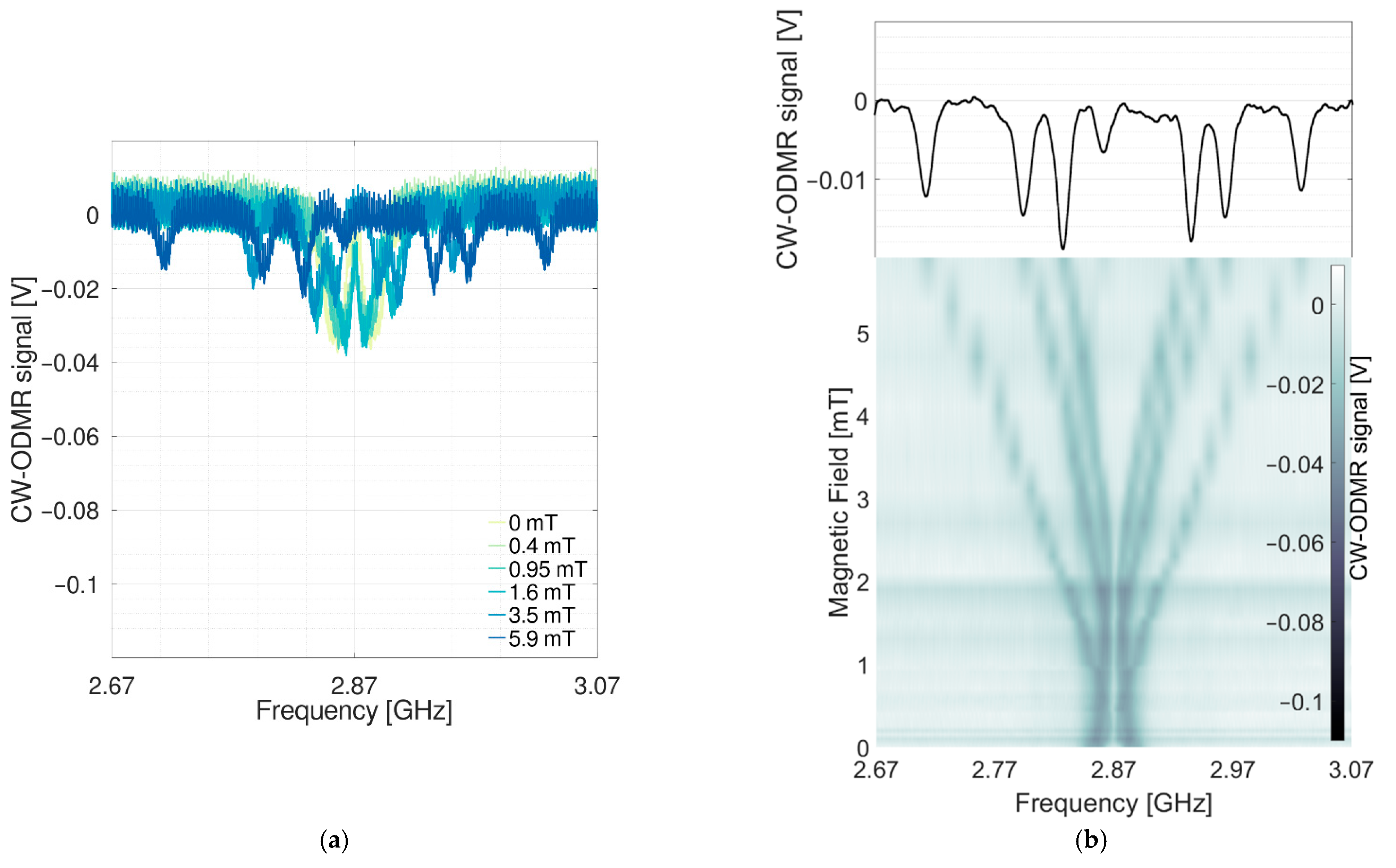
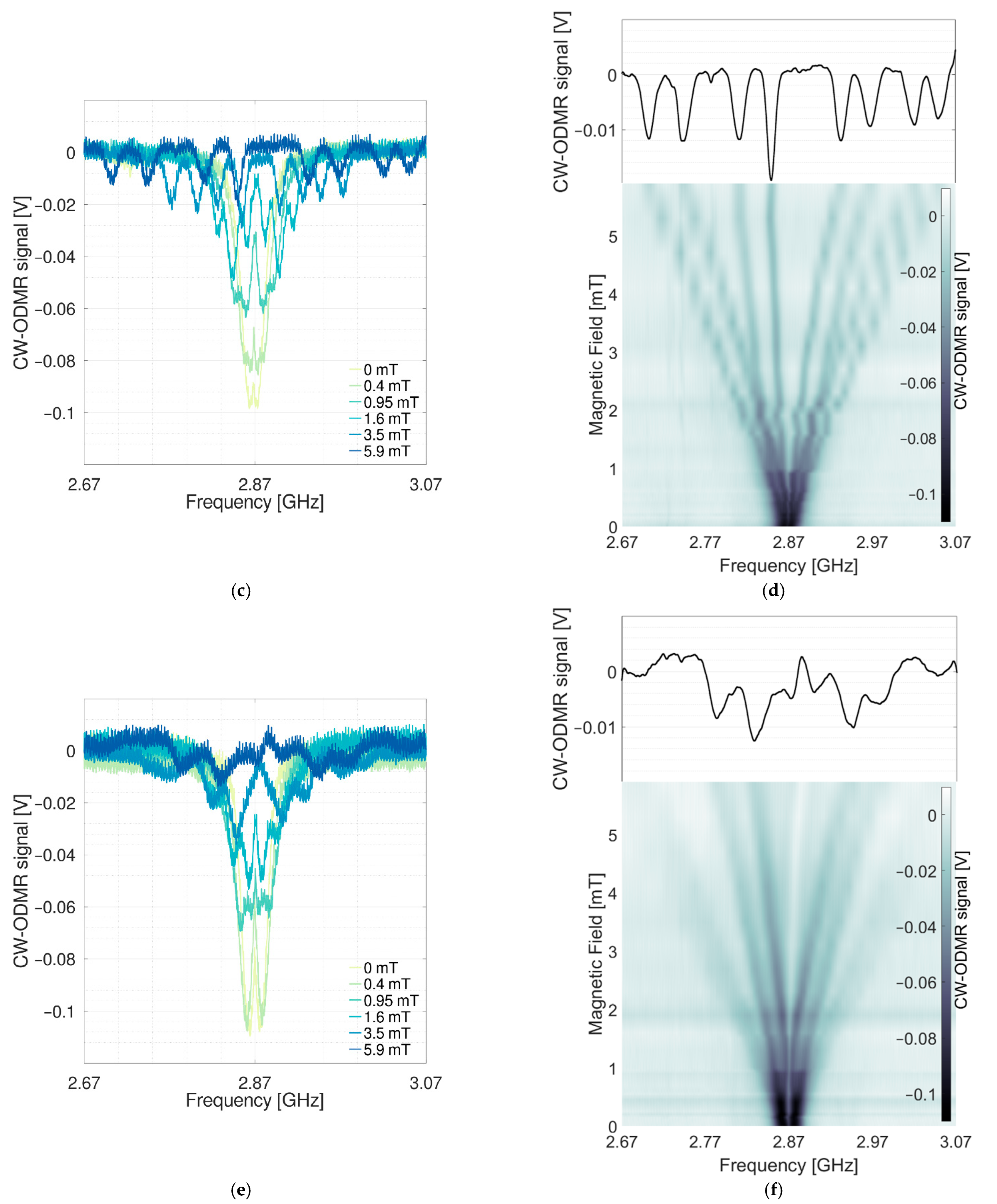
3.6. CW-ODMR Signals
4. Discussion
5. Conclusions
Author Contributions
Funding
Data Availability Statement
Conflicts of Interest
Abbreviations
| ADC | Analog-to-digital converter |
| COTS | Commercial off-the-shelf |
| CVD | Chemical vapor deposition |
| CW | Continuous wave |
| FWHM | Full width at half maximum |
| GPSDO | Global positioning system disciplined oscillator |
| HPHT | High pressure, high temperature |
| LED | Light-emitting diode |
| MW | Microwave |
| NV | Nitrogen-vacancy |
| ODMR | Optically detected magnetic resonance |
| OPM | Optically pumped magnetometers |
| PC | Personal computer |
| SNR | Signal-to-noise ratio |
| SQUIDs | Superconductive quantum interference devices |
| TIA | Transimpedance amplifier |
| VNA | Vector network analyzer |
| ZFS | Zero-field splitting |
Appendix A

| Component | Description or Part Number | Supplier | Quantity | Price per Piece [EUR] | Price per Sales Unit [EUR] |
|---|---|---|---|---|---|
| Constant current source | LUMITRONIX Micro-Konstantstromquelle | www.leds.de | 1 | 0.99 | |
| LED | C503B-GCN-CY0C0792 or C503B-GCN-CY0C0791 | RS Components | 1 | 0.30 | |
| Microdiamond | MDNV150umHi30mg | Adámas Nanotechnologies | 1 | ~3 | 578 (30 mg) |
| Color filter | LEE 027 MEDIUM RED | Thomann | 1 (4.5 × 4.0 mm2) | <0.01 | 5.50 (per role) |
| Photodiode | BPW34 | RS Components | 1 | 1.20 | |
| Optical adhesive | NOA61 | Thorlabs | 40.75 (bottle with 1 oz.) | ||
| Microwave generator board | ADF435 | ebay | 1 | ~30 | |
| SMA connector | Amphenol RF 132289 | RS Components | 2 | 10.60 | |
| Capacitor 1 pF | VJ0603D1R0BXPAJ | RS Components | 1 | 0.32 | |
| Copper wire | Ø 0.2 mm | 1 | |||
| Angled SMA connector | RS Pro | RS Components | 1 | 17.05 | |
| Termination resistor | Amphenol RF 132360 | RS Components | 1 | 5.87 | |
| Operational amplifier | OPA140 | RS Components | 1 | 4.26 | |
| Passives components for TIA | Resistors, capacitors, connectors | RS Components | |||
| NV-magnetometer | All listed components | 1 | ~74 |
References
- Zhang, H.; Belvin, C.; Li, W.; Wang, J.; Wainwright, J.; Berg, R.; Bridger, J. Little bits of diamond: Optically detected magnetic resonance of nitrogen-vacancy centers. Am. J. Phys. 2018, 86, 225–236. [Google Scholar] [CrossRef]
- Pogorzelski, J.; Horsthemke, L.; Homrighausen, J.; Stiegekötter, D.; Gregor, M.; Glösekötter, P. Compact and Fully Integrated LED Quantum Sensor Based on NV Centers in Diamond. Sensors 2024, 24, 743. [Google Scholar] [CrossRef]
- Zheng, D.; Ma, Z.; Guo, W.; Niu, L.; Wang, J.; Chai, X.; Li, Y.; Sugawara, Y.; Yu, C.; Shi, Y.; et al. A hand-held magnetometer based on an ensemble of nitrogen-vacancy centers in diamond. J. Phys. D Appl. Phys. 2020, 53, 155004. [Google Scholar] [CrossRef]
- Stegemann, J.; Peters, M.; Horsthemke, L.; Langels, N.; Glösekötter, P.; Heusler, S.; Gregor, M. Modular low-cost 3D printed setup for experiments with NV centers in diamond. Eur. J. Phys. 2023, 44, 35402. [Google Scholar] [CrossRef]
- Stürner, F.M.; Brenneis, A.; Buck, T.; Kassel, J.; Rölver, R.; Fuchs, T.; Savitsky, A.; Suter, D.; Grimmel, J.; Hengesbach, S.; et al. Integrated and Portable Magnetometer Based on Nitrogen-Vacancy Ensembles in Diamond. Adv. Quantum Tech. 2021, 4, 2000111. [Google Scholar] [CrossRef]
- Acosta, V.M.; Bauch, E.; Ledbetter, M.P.; Waxman, A.; Bouchard, L.S.; Budker, D. Temperature dependence of the nitrogen-vacancy magnetic resonance in diamond. Phys. Rev. Lett. 2010, 104, 070801. [Google Scholar] [CrossRef] [PubMed]
- Fan, Z.; Xing, L.; Wu, F.; Feng, X.; Zhang, J. The Optimization of Microwave Field Characteristics for ODMR Measurement of Nitrogen-Vacancy Centers in Diamond. Photonics 2024, 11, 436. [Google Scholar] [CrossRef]
- Tabuchi, H.; Matsuzaki, Y.; Furuya, N.; Nakano, Y.; Watanabe, H.; Tokuda, N.; Mizuochi, N.; Ishi-Hayase, J. Temperature sensing with RF-dressed states of nitrogen-vacancy centers in diamond. J. Appl. Phys. 2023, 133, 024401. [Google Scholar] [CrossRef]
- Dolde, F.; Fedder, H.; Doherty, M.W.; Nöbauer, T.; Rempp, F.; Balasubramanian, G.; Wolf, T.; Reinhard, F.; Hollenberg, L.C.L.; Jelezko, F.; et al. Electric-field sensing using single diamond spins. Nat. Phys. 2011, 7, 459–463. [Google Scholar] [CrossRef]
- Michl, J.; Steiner, J.; Denisenko, A.; Bülau, A.; Zimmermann, A.; Nakamura, K.; Sumiya, H.; Onoda, S.; Neumann, P.; Isoya, J.; et al. Robust and Accurate Electric Field Sensing with Solid State Spin Ensembles. Nano Lett. 2019, 19, 4904–4910. [Google Scholar] [CrossRef]
- Yang, B.; Murooka, T.; Mizuno, K.; Kim, K.; Kato, H.; Makino, T.; Ogura, M.; Yamasaki, S.; Schmidt, M.E.; Mizuta, H.; et al. Vector Electrometry in a Wide-Gap-Semiconductor Device Using a Spin-Ensemble Quantum Sensor. Phys. Rev. Appl. 2020, 14, 044049. [Google Scholar] [CrossRef]
- Doherty, M.W.; Manson, N.B.; Delaney, P.; Jelezko, F.; Wrachtrup, J.; Hollenberg, L.C. The nitrogen-vacancy colour centre in diamond. Phys. Rep. 2013, 528, 1–45. [Google Scholar] [CrossRef]
- Jelezko, F.; Wrachtrup, J. Single defect centres in diamond: A review. Phys. Status Solidi (A) 2006, 203, 3207–3225. [Google Scholar] [CrossRef]
- Homrighausen, J.; Horsthemke, L.; Pogorzelski, J.; Trinschek, S.; Glösekötter, P.; Gregor, M. Edge-Machine-Learning-Assisted Robust Magnetometer Based on Randomly Oriented NV-Ensembles in Diamond. Sensors 2023, 23, 1119. [Google Scholar] [CrossRef]
- Abe, E.; Sasaki, K. Tutorial: Magnetic resonance with nitrogen-vacancy centers in diamond—Microwave engineering, materials science, and magnetometry. J. Appl. Phys. 2018, 123, 161101. [Google Scholar] [CrossRef]
- Sánchez Toural, J.L.; Marzoa, V.; Bernardo-Gavito, R.; Pau, J.L.; Granados, D. Hands-On Quantum Sensing with NV−Centers in Diamonds. C 2023, 9, 16. [Google Scholar] [CrossRef]
- Mariani, G.; Umemoto, A.; Nomura, S. A home-made portable device based on Arduino Uno for pulsed magnetic resonance of NV centers in diamond. AIP Adv. 2022, 12, 065321. [Google Scholar] [CrossRef]
- Soshenko, V.V.; Bolshedvorskii, S.V.; Rubinas, O.; Sorokin, V.N.; Smolyaninov, A.N.; Vorobyov, V.V.; Akimov, A.V. Nuclear Spin Gyroscope based on the Nitrogen Vacancy Center in Diamond. Phys. Rev. Lett. 2021, 126, 197702. [Google Scholar] [CrossRef]
- Chatzidrosos, G.; Wickenbrock, A.; Bougas, L.; Leefer, N.; Wu, T.; Jensen, K.; Dumeige, Y.; Budker, D. Miniature Cavity-Enhanced Diamond Magnetometer. Phys. Rev. Appl. 2017, 8, 044019. [Google Scholar] [CrossRef]
- Zhang, C.; Shagieva, F.; Widmann, M.; Kübler, M.; Vorobyov, V.; Kapitanova, P.; Nenasheva, E.; Corkill, R.; Rhrle, O.; Nakamura, K.; et al. Diamond Magnetometry and Gradiometry Towards Subpicotesla dc Field Measurement. Phys. Rev. Appl. 2021, 15, 064075. [Google Scholar] [CrossRef]
- Wang, X.; Zheng, D.; Wang, X.; Liu, X.; Wang, Q.; Zhao, J.; Guo, H.; Qin, L.; Tang, J.; Ma, Z.; et al. Portable Diamond NV Magnetometer Head Integrated With 520 nm Diode Laser. IEEE Sens. J. 2022, 22, 5580–5587. [Google Scholar] [CrossRef]
- Sasaki, K.; Monnai, Y.; Saijo, S.; Fujita, R.; Watanabe, H.; Ishi-Hayase, J.; Itoh, K.M.; Abe, E. Broadband, large-area microwave antenna for optically-detected magnetic resonance of nitrogen-vacancy centers in diamond. Rev. Sci. Instrum. 2016, 87, 134. [Google Scholar] [CrossRef]
- Herrmann, J.; Appleton, M.A.; Sasaki, K.; Monnai, Y.; Teraji, T.; Itoh, K.M.; Abe, E. Polarization- and frequency-tunable microwave circuit for selective excitation of nitrogen-vacancy spins in diamond. Appl. Phys. Lett. 2016, 109, 134. [Google Scholar] [CrossRef]
- Bayat, K.; Choy, J.; Baroughi, M.F.; Meesala, S.; Loncar, M. Efficient, uniform, and large area microwave magnetic coupling to NV centers in diamond using double split-ring resonators. Nano Lett. 2014, 14, 1208–1213. [Google Scholar] [CrossRef] [PubMed]
- Kuwahata, A.; Kitaizumi, T.; Saichi, K.; Sato, T.; Igarashi, R.; Ohshima, T.; Masuyama, Y.; Iwasaki, T.; Hatano, M.; Jelezko, F.; et al. Magnetometer with nitrogen-vacancy center in a bulk diamond for detecting magnetic nanoparticles in biomedical applications. Sci. Rep. 2020, 10, 2483. [Google Scholar] [CrossRef] [PubMed]
- Johansson, S.; Lönard, D.; Barbosa, I.C.; Gutsche, J.; Witzenrath, J.; Widera, A. A miniaturized magnetic field sensor based on nitrogen-vacancy centers. arXiv 2024, arXiv:2402.19372v3. [Google Scholar] [CrossRef]
- Stürner, F.M.; Brenneis, A.; Kassel, J.; Wostradowski, U.; Rölver, R.; Fuchs, T.; Nakamura, K.; Sumiya, H.; Onoda, S.; Isoya, J.; et al. Compact integrated magnetometer based on nitrogen-vacancy centres in diamond. Diam. Relat. Mater. 2019, 93, 59–65. [Google Scholar] [CrossRef]
- Abrahams, G.J.; Ellul, E.; Robertson, I.O.; Khalid, A.; Greentree, A.D.; Gibson, B.C.; Tetienne, J.-P. Handheld device for non-contact thermometry via optically detected magnetic resonance of proximate diamond sensors. Phys. Rev. Appl. 2023, 19, 054076. [Google Scholar] [CrossRef]
- Hu, Q.; Huang, K.; Mao, X.; Ran, G.; He, X.; Lin, Z.; Hu, T.; Ran, S. Design of high sensitivity magnetometer based on Diamond Nitrogen-Vacancy Centers and Weak Signal Output Module. Diam. Relat. Mater. 2025, 151, 111858. [Google Scholar] [CrossRef]
- Deguchi, H.; Hayashi, T.; Saito, H.; Nishibayashi, Y.; Teramoto, M.; Fujiwara, M.; Morishita, H.; Mizuochi, N.; Tatsumi, N. Compact and portable quantum sensor module using diamond NV centers. Appl. Phys. Express 2023, 16, 62004. [Google Scholar] [CrossRef]
- Webb, J.L.; Clement, J.D.; Troise, L.; Ahmadi, S.; Johansen, G.J.; Huck, A.; Andersen, U.L. Nanotesla sensitivity magnetic field sensing using a compact diamond nitrogen-vacancy magnetometer. Appl. Phys. Lett. 2019, 114, 231103. [Google Scholar] [CrossRef]
- Duan, D.; Du, G.X.; Kavatamane, V.K.; Arumugam, S.; Tzeng, Y.-K.; Chang, H.-C.; Balasubramanian, G. Efficient nitrogen-vacancy centers’ fluorescence excitation and collection from micrometer-sized diamond by a tapered optical fiber in endoscope-type configuration. Opt. Express 2019, 27, 6734–6745. [Google Scholar] [CrossRef]
- Fedotov, I.V.; Doronina-Amitonova, L.V.; Voronin, A.A.; Levchenko, A.O.; Zibrov, S.A.; Sidorov-Biryukov, D.A.; Fedotov, A.B.; Velichansky, V.L.; Zheltikov, A.M. Electron spin manipulation and readout through an optical fiber. Sci. Rep. 2014, 4, 5362. [Google Scholar] [CrossRef] [PubMed]
- Chen, F.L.; Huang, S.K.; Jiang, T.J.; Yan, F.S. Utilizing a homemade handheld magnetometer to sense nanotesla magnetic fields. Res. Sq. 2023. [Google Scholar] [CrossRef]
- Qin, L.; Fu, Y.; Zhang, S.; Zhao, J.; Gao, J.; Yuan, H.; Ma, Z.; Shi, Y.; Liu, J. Near-field microwave radiation function on spin assembly of nitrogen vacancy centers in diamond with copper wire and ring microstrip antennas. Jpn. J. Appl. Phys. 2018, 57, 72201. [Google Scholar] [CrossRef]
- Fedotov, I.V.; Blakley, S.M.; Serebryannikov, E.E.; Hemmer, P.; Scully, M.O.; Zheltikov, A.M. High-resolution magnetic field imaging with a nitrogen-vacancy diamond sensor integrated with a photonic-crystal fiber. Opt. Lett. 2016, 41, 472–475. [Google Scholar] [CrossRef]
- Don Klipstein. C.I.E. Photopic Luminous Efficiency Function. Available online: https://donklipstein.com/photopic.html (accessed on 10 July 2025).
- Ruiz, A.J.; Giallorenzi, M.K.; Hunt, B.; Samkoe, K.S.; Pogue, B.W. Lighting gel filters as low-cost alternatives for fluorescence imaging and optical system design. Opt. Eng. 2022, 61, 085103. [Google Scholar] [CrossRef]
- Montalti, M.; Cantelli, A.; Battistelli, G. Nanodiamonds and silicon quantum dots: Ultrastable and biocompatible luminescent nanoprobes for long-term bioimaging. Chem. Soc. Rev. 2015, 44, 4853–4921. [Google Scholar] [CrossRef]
- Würth Elektronik eiSos GmbH & Co., KG. WL-SMTW SMT Mono-Color TOP LED Waterclear: Order Code: 150224GS73100. Available online: https://www.we-online.com/components/products/datasheet/150224GS73100.pdf (accessed on 10 July 2025).
- Cree, Inc. Cree® 5-mm Blue and Green Round LED C503B-BCS/BCN/GCS/GCN. Available online: https://www.farnell.com/datasheets/1975638.pdf (accessed on 10 July 2025).
- O’Haver, T. Smoothing. Available online: https://terpconnect.umd.edu/~toh/spectrum/Smoothing.html (accessed on 19 May 2025).
- Omar, M.; Conta, A.; Westerhoff, A.; Hasse, R.; Chatzidrosos, G.; Budker, D.; Wickenbrock, A. Diamond-optic enhanced photon collection efficiency for sensing with nitrogen-vacancy centers. Opt. Lett. 2023, 48, 2512. [Google Scholar] [CrossRef]
- Zhang, S.; Ma, Z.; Qin, L.; Fu, Y.; Shi, Y.; Liu, J.; Li, Y.J. Fluorescence detection using optical waveguide collection device with high efficiency on assembly of nitrogen vacancy centers in diamond. Appl. Phys. Express 2018, 11, 13007. [Google Scholar] [CrossRef]
- Reedu GmbH & Co., KG. senseBox: Your Toolkit for Digital Education, Citizen Science and Environmental Monitoring. Available online: https://sensebox.de/en/ (accessed on 10 July 2025).
- Reedu GmbH & Co., KG. QOOOL Sensing—Quantum Sensing for Digital Education. Available online: https://qoool-sensing.org/en (accessed on 10 July 2025).


| Properties | LED1 | LED2 | LED3 |
|---|---|---|---|
| Package | SMD * | 5 mm THT ** | SMD * |
| Continuous Forward Current [mA] | 30 | 30 | 70 |
| Operating Temperature [°C] | −40 … +85 | −40 … +95 | −40 … +100 |
| Peak Wavelength [nm] | 519 1 | - | 515 2 |
| Dominant Wavelength [nm] | 528 1 | 527 1 | 520 2 |
| Luminous Intensity [mcd] | Typ. 1200 1 | Typ. 20,000 1 | Typ. 30,000 2 |
| Spectral Bandwidth [nm] | 30 1 | - | 40 2 |
| Viewing Angle Phi 0° [°] | 120 1 | 30 1 | 30 2 |
| Properties | LED1 | LED2 | LED3 |
|---|---|---|---|
| Solid Angle [sr] | 3.1416 | 0.2141 | 0.2141 |
| Luminous Flux [lm] | 3.77 1 | 4.28 1 | 6.42 2 |
| C.I.E. Photopic Luminous Efficiency Function | 0.8363 | 0.82249 | 0.71 |
| Optical Power [mW] | 6.6 1 | 7.6 1 | 13.2 2 |
| Build | Resistor (kΩ) | Capacitor (F) |
|---|---|---|
| LED3 + microdiamond | 620 | 120 p |
| LED3 + large HPHT diamond | 56 | 12 n |
| LED2 shortened + large HPHT diamond | 82 | 8.2 n |
| Build | ZFS (MHz) | FWHM (MHz) |
|---|---|---|
| LED3 + microdiamond | 31 | 13 |
| LED3 + large HPHT diamond | 9 | 15 |
| LED2 shortened + large HPHT diamond | 11 | 23 |
Disclaimer/Publisher’s Note: The statements, opinions and data contained in all publications are solely those of the individual author(s) and contributor(s) and not of MDPI and/or the editor(s). MDPI and/or the editor(s) disclaim responsibility for any injury to people or property resulting from any ideas, methods, instructions or products referred to in the content. |
© 2025 by the authors. Licensee MDPI, Basel, Switzerland. This article is an open access article distributed under the terms and conditions of the Creative Commons Attribution (CC BY) license (https://creativecommons.org/licenses/by/4.0/).
Share and Cite
Bülau, A.; Walter, D.; Fritz, K.-P. Components for an Inexpensive CW-ODMR NV-Based Magnetometer. Magnetism 2025, 5, 18. https://doi.org/10.3390/magnetism5030018
Bülau A, Walter D, Fritz K-P. Components for an Inexpensive CW-ODMR NV-Based Magnetometer. Magnetism. 2025; 5(3):18. https://doi.org/10.3390/magnetism5030018
Chicago/Turabian StyleBülau, André, Daniela Walter, and Karl-Peter Fritz. 2025. "Components for an Inexpensive CW-ODMR NV-Based Magnetometer" Magnetism 5, no. 3: 18. https://doi.org/10.3390/magnetism5030018
APA StyleBülau, A., Walter, D., & Fritz, K.-P. (2025). Components for an Inexpensive CW-ODMR NV-Based Magnetometer. Magnetism, 5(3), 18. https://doi.org/10.3390/magnetism5030018