A Study on the Effect of Plastic Strain on Magnetic Phenomenology and Microstructure

Abstract

The present work aspires to contribute to the discussion on the relationship between macroscopic measurements and microstructure, helping establish a methodology that will allow the quantitative assessment of the effect of strain on magnetic properties in the plastic deformation regime. In particular, we study the effect of strain on the magnetization process as a result of varying the anisotropy profile at the grain level. Results on micromagnetic calculations of hysteresis loops for various configurations of magnetic anisotropy are shown and discussed against the interplay between the energy terms involved in the calculations, namely anisotropy, demagnetizing, and exchange. The results are in line with previously obtained results using vector Preisach modeling with the Stoner–Wohlfarth model acting both as a switching and rotation mechanism. The hysteresis loop phenomenology is consistent with the emergence of a hard phase in the form of a boundary around soft grains which is assumed to be the result of the onset of compressive stresses in the plastic region. Future research will be oriented toward the study of the effect of the secondary peak in differential permeability, which is observed experimentally in the plastic deformation region, and its dependence on the angle of misalignment between the hard boundary and the soft grain.

1. Introduction

Nondestructive testing and evaluation (NDT&E) techniques are important both for the monitoring of critical structures as well as for zero-defect manufacturing. In particular, magnetic NDT&E is one of the most promising technologies where magnetic materials are involved, as in the case of steel structures and the steel manufacturing industry.

The underlying concept of magnetic NDT&E is the dependence of the magnetization process on strain. Mechanical stresses applied at the manufacturing stage, mechanical and thermal treatments, loading, and aging during the lifetime of a material are all causes of strain which manifests itself as deformation at the lattice, grain, or macroscopic level and results in residual stresses [1].

These techniques fall under two major categories, namely those based on major or minor loop measurements [2,3,4,5,6] and those based on magnetic Barkhausen noise [7,8,9,10,11] measurements. Coercivity, remanence, and magnetic permeability are all properties that have been proposed as metrics in the first case, while the noise root mean square (rms) voltage envelope, counts or energy are proposed for the second category.

Magnetic NDT&E techniques are appealing due to the low-cost sensor arrangements and their adaptability to various applications in the field, which is most important for both monitoring and manufacturing uses. However, it often suffers from drawbacks, such as low repeatability as well as a lack of benchmarking and standardization, which makes it appropriate for qualitative rather than quantitative assessment [6,11,12,13,14].

Modeling the effect of strain on the magnetization process is important for understanding the underlying mechanisms governing the dependence of the measured/monitored magnetic parameters on microstructural changes related to strain and residual stresses.

The modeling of stress-dependent magnetization processes has been studied by a number of groups at various scales [15,16,17,18]. The stress tensor contributes to the effective magnetic field distribution in a strained magnetic material and affects the magnetization reversal mechanism; e.g., when a tensile (positive) stress is applied along the dominant magnetization axis of a sample with positive magnetostriction, it assists the alignment of the domains with the dominant magnetization direction, whereas if compressive (negative) stress is applied, the domains tend to rotate away from the dominant magnetization direction. This approach has been used in a modification of the Jiles–Atherton model [19]. The effect of stress and/or microstructure in order to make better predictions on the efficiency and performance of different electrical machines has been modeled for several applications: the effect of grain size and dislocation density on hysteretic magnetic properties in steels [19], the influence of biaxial stress on anhysteretic behavior [20], strain broadening under the effect of dislocations [21], asymmetry in the magnetomechanical effect under tensile and compressive stress [22], and the effect of multiaxial stress on magnetic hysteresis of electrical steel sheets [23].

The stress-depending effective field approach is not as straightforward in the case of plastically deformed materials in the unloaded state where compressive stresses coexist with tensile stresses and the stress tensor is not known.

In this work, we aspire to contribute to the discussion on the relationship between macroscopic measurements and microstructure on the way toward establishing a methodology that will allow the quantitative assessment of the effect of strain on magnetic properties in the plastic deformation regime. Our starting point is experimental evidence and previous modeling results concerning martensitic steels [15]. Tensile stress in the plastic deformation regime results in the emergence of compressive residual stresses and a magnetically hard phase in the grain boundaries [1,24]. This is reflected on hysteresis loops with increased coercivity as well as lower remanence and differential permeability. This phenomenology has been reproduced by a modeling approach based on the Preisach formalism which assumes the existence of a hard phase and stress-dependent long-range interactions, i.e., magnetostatic energy increasing with strain [15]. In this work, we treat the effect of strain on the magnetization process in the plastic deformation regime as a result of a varying anisotropy profile at the grain level, and more specifically, we consider the emergence of a magnetic hard phase in the form of a grain boundary. Using the open-source software OOMMF 1.2b2 [25,26] and the energy minimization approach, major loops are calculated for various configurations, and the interplay between the energy terms involved is studied.

In the following section, we present the materials and experimental evidence on which our work is based, and we describe the proposed methodology. In Section 3, we present the simulation results and their discussion, and the conclusions are presented in Section 4 and Section 5, respectively.

2. Materials and Methods

The assumptions of the modeling approach presented in this work originate from observations on experimental results. In particular, the measurements shown here have been obtained using commercial electrical steel laminates, featuring a low-carbon steel typically used as the magnetic core in transformers and motors and typical of similar measurements in the literature [1,2,4,10,11,14,27]. Samples 30 mm × 3 mm cut from the same 0.5 mm sheet [2] have been used.

Three types of measurements are used to study the response of the sample to applied magnetic fields as well as to applied and residual stresses. First, stress–strain curves (Figure 1) have been obtained at three different rates of applied stress, namely 0.1 mm/min, 0.5 mm/min, and 1 mm/min, using an INSTRON 8800 machine. The stress–strain curve is used to establish the ranges of the elastic and plastic regions of the samples used in this study. The transition to the plastic region is observed at strain levels exceeding 3%.

During the stress–strain curve measurement, a sensor monitoring the magnetic Barkhausen noise (mBN), as described in [26], was also attached to the sample. The excitation is provided by a triangular waveform at 10 Hz. The magnetic field is applied along the same direction as the applied stress. The mBN counts (using MagLab MEB2c) exceeding a specific threshold are used as the mBN metric of choice [11] in Figure 1. Similar results are obtained when the mBN voltage is used instead. The effect applied stress on mBN counts is directly linked to the effect of stress on strain. This measurement demonstrates the coupling between magnetic and mechanical properties and the potential of magnetic macroscopic parameters for the monitoring of mechanical properties such as strain. The transition to the plastic region at strains higher than 3% is also observed in the mBN measurements.

The third type of measurement concerns hysteresis loop measurements using AC magnetometry where an excitation coil wrapped around a yoke [26] generates a low frequency < 0.5 Hz sinusoidal field and magnetizes the sample [2,6,11]. A sensing coil wound around the sample measures the induced output voltage which is proportional to the differential permeability of the material in the volume enclosed by the sensing coil. The hysteresis loops (Figure 2) are obtained on unloaded strained samples to study the effect of residual stress on the magnetization process; first, tensile stress is applied on the sample using the 0.5 mm/min strain rate up to a given strain level. Then, the sample is unloaded, and the hysteresis loop is measured. The magnetic field is applied along the direction the stress has been previously applied, namely along the length of the sample. The hysteresiograph is an inhouse device which has not been calibrated, hence the use a.u.

In the plastic deformation regime, there is a monotonic dependence of coercivity and differential permeability on strain. Coercivity increases and permeability decreases. At the microstructural level, higher plastic strain is related to more, finer and misaligned grains and the emergence and development of a hard phase around soft grains, which is the result of the compressive residual stresses that set in [1,24]. The coercivity increase is explained as a result of the hard phase which increases with strain in the plastic region and increased domain wall pinning due to misaligned grains and longer grain boundaries. The decrease in differential permeability is attributed to the emergence of hard boundaries, as the result of compressive residual stresses, whose effective anisotropy is transverse or not aligned with the direction of tensile stress which caused the plastic deformation.

In our previous work, a Preisach model was constructed which used the Stoner–Wohlfarth mechanism as a 2D vector hysteresis operator allowing for both reversible and irreversible rotation and assumed a dispersion of anisotropy around a main easy direction. The emergence of the hard magnetic phase was introduced via secondary Preisach density functions and long-range interactions [15].

Based on the conclusions drawn from both experimental and modeling results, we use the OOMMF open-source software [25] to model the effect of microstructure on the hysteresis loop computed as the result of the free energy minimization for each applied field value. The total energy for a given applied field value is the sum of the Zeeman, anisotropy, exchange, and magnetostatic energy terms.

The reason for this approach is that in engineering applications, the measured parameters involved in the NDT&E of systems containing magnetic materials are usually those obtained from a major loop: e.g., coercivity, remanence, differential permeability, etc. As explained in the Introduction, the goal is to eventually correlate macroscopic parameters obtained from major loop measurements to microstructural changes related to strain. The effect of strain is modeled indirectly through microstructural configurations involving more than one magnetic phase.

In order to study the effect of microstructure and magnetic parameters on the phenomenology depicted by the major loop calculation, the following approach has been designed.

The assumptions of the simulated experiments are outlined below:

• The sample studied (Figure 3) is a parallelpiped of dimensions $L\times L\times H {\left(\mathrm{n}\mathrm{m}\right)}^3$. $L$ is in the order of $2000 \mathrm{n}\mathrm{m}$ and $H$ is at least two orders of magnitude smaller.
• It is discretized in N cubic cells of side a nm. N is determined by the sample dimensions and the cell size by dividing each side of the sample with the parameter a. The cell size depends on the magnetostatic exchange length for the soft magnetic materials and monocrystalline exchange length for the hard magnetic materials, which are determined by the material parameters $M_S,K_1,$ and/or $A_{ex}$, namely, the saturation magnetization, anisotropy constant and exchange constant, respectively.
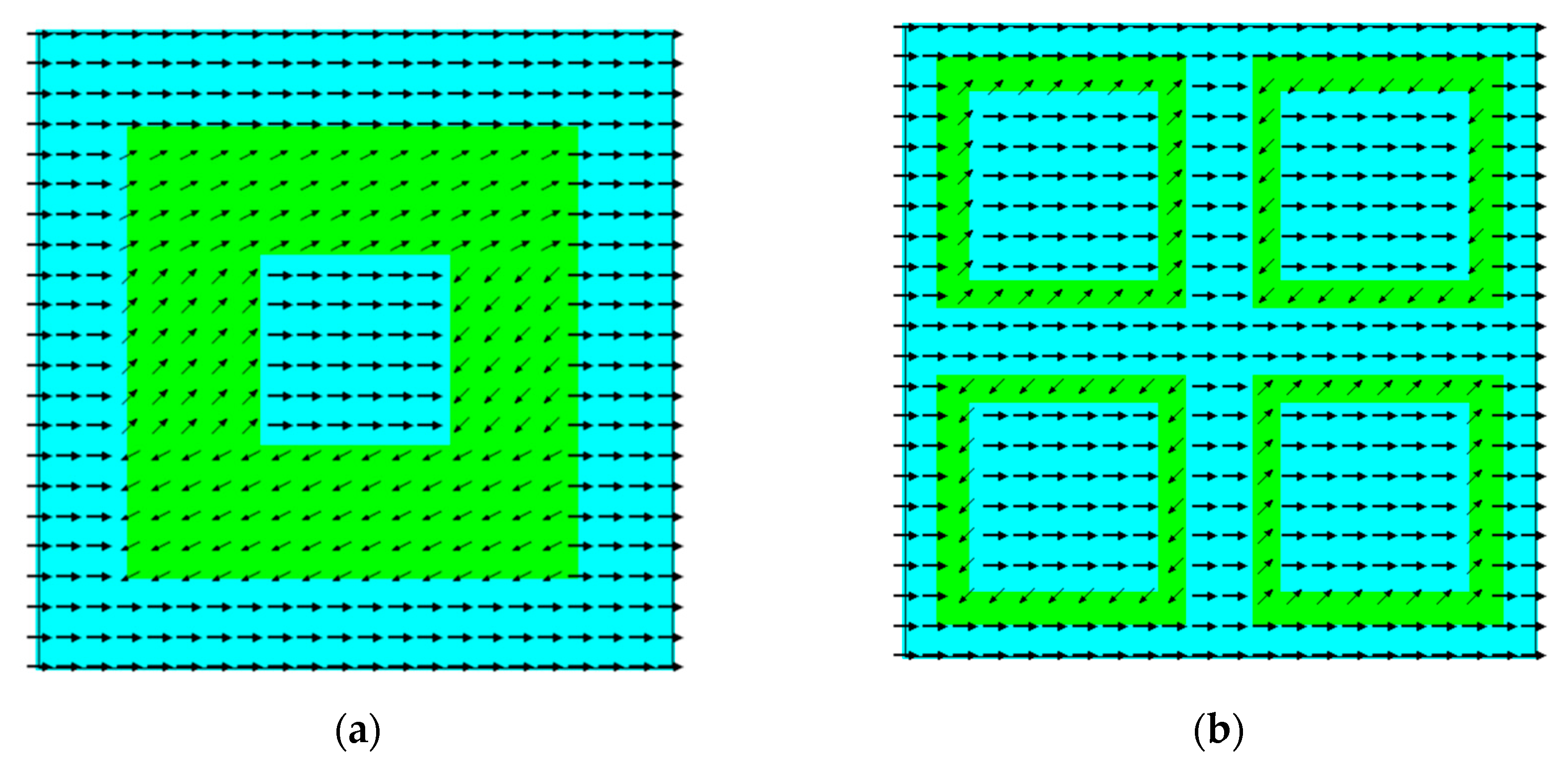
• Each cell represents one magnetic dipole with parameters $M_S,K_1,$ and/or $A_{ex}$. Figure 4 shows typical magnetization plots generated by the software of a soft magnetic matrix and soft grains enclosed by misaligned hard boundaries.

Several simulation experiments have been performed to study the effect of microstructure on the major loop, e.g., hard inclusions in a soft matrix, hard inclusions and voids, and finally soft grains surrounded by misaligned hard boundaries [13,14,15] as those depicted in Figure 4, which is closer to what is reported in experimental studies. The geometries of the models presented in Figure 4a,b serve as initial conditions of the simulations presented in

Table 1. Simulation parameters of the configurations shown in Figure 4.

#	Configuration	${\mathit{K}}_1$—Magnitude $[\mathbf{J}/{\mathbf{m}}^3$]	${\mathit{K}}_1$—Direction [x y z]	${\mathit{A}}_{\mathit{e}\mathit{x}}$$, [\mathbf{J}/\mathbf{m}$]	${\mathit{M}}_{\mathit{S}}$—Magnitude $[\mathbf{A}/\mathbf{m}$]	Applied Field [mT] [x y z]
1	Homogeneous case	Ignore	1 0 0	1.30 × 10−11	1.70 × 106	[1000 0 0]
2	4 hard grain boundaries	4.80 × 103	1 0 0	1.30 × 10−11	1.70 × 106	[1000 1000 0]
		1.00 × 106	1 1 0	1.30 × 10−11	1.40 × 106
3	4 hard grain boundaries	4.80 × 103	1 0 0	1.30 × 10−11	1.70 × 106	[1000 0 0]
		1.00 × 106	1 1 0	1.30 × 10−11	1.40 × 106
4	4 hard grain boundaries	4.80 × 103	1 0 0	2.10 × 10−11	1.70 × 106	[1000 1000 0]
		1.00 × 106	1 1 0	1.30 × 10−11	1.40 × 106
5	4 hard grain boundaries	4.80 × 103	1 0 0	2.10 × 10−11	1.70 × 106	[1000 1000 0]
		1.00 × 106	1 1 0	2.10 × 10−11	1.40 × 106
6	1 hard (thin) grain boundary	4.80 × 103	1 0 0	1.30 × 10−11	1.70 × 106	[1000 1000 0]
		1.00 × 106	1 1 0	1.30 × 10−11	1.40 × 106
7	1 hard (thick) grain boundary: 179200 hard cells	4.80 × 103	1 0 0	1.30 × 10−11	1.70 × 106	[1000 1000 0]
		1.00 × 106	1 1 0	1.30 × 10−11	1.40 × 106
8	1 hard (thick) grain boundary: 179200 hard cells	4.80 × 103	1 0 0	1.30 × 10−11	1.70 × 106	[1000 1000 0]
		5.00 × 105	1 1 0	1.30 × 10−11	1.40 × 106
9	1 hard grain boundary _179200hardcells_topbottomYdir	4.80 × 103	1 0 0	1.30 × 10−11	1.70 × 106	[1000 1000 0]
		1.00 × 106	1 1 0 0 1 0	1.30 × 10−11	1.40 × 106
10	1 hard grain boundary _179200hardcells_topbottomstrongerx	4.80 × 103	1 0 0	1.30 × 10−11	1.70 × 106	[1000 1000 0]
		1.00 × 106	1 1 0 1 0.5 0	1.30 × 10−11	1.40 × 106
11	1 hard grain boundary _179200hardcells_topbottomstrongerx_Hxdir	4.80 × 103	1 0 0	1.30 × 10−11	1.70 × 106	[1000 0 0]
		1.00 × 106	1 1 0 1 0.5 0	1.30 × 10−11	1.40 × 106

, (#2–#5) and (#6–#11), respectively. Material parameters were changed to study the effects on the hysteresis loop as explained later in the paper and presented in Table 1.

In the energy minimization approach, the magnetization process is the result of the interplay between the energy terms involved, namely the exchange, anisotropy and magnetostatic energy densities, and the applied field. Therefore, we focus on the effect of microstructural parameters on the energy terms involved.

3. Results

The results reported here concern the geometry shown in Figure 4. The simulation parameters for these results are summarized in Table 1. In the column “Configuration”, we present different simulations studies: homogeneous case, different cases that include four soft grains (#2–#5) with hard boundaries in a soft matrix (“4 hard grain boundaries”), and the cases with one soft grain (#6–#11) with hard boundaries in a soft matrix (“1 hard (thick) grain boundary”). The presented case with the four soft grains is then examined more through changing the value of the exchange energy coefficient (A [pJ/m]) and the direction of the applied field to observe the effect of the exchange energy coefficient and the applied field on the hysteresis. Then, to observe the effect of the geometry of the soft grains, we have simulated a sample with only one soft grain with hard boundaries where we observed one scenario when the hard boundary is thin (#6), and the rest of the cases are with thick boundaries (#6–#11) keeping the same number of the hard cells in the grain boundary (179,200 hard cells) as used in (#2–#5). Furthermore, we used different anisotropy profiles in the top and bottom part of the boundary by changing the direction of the anisotropy in those sections (#9–#11), while the sides of the hard grain boundary remain the same. The direction of the anisotropy in the mentioned cases is indicated in the name of the configuration; i.e., (#9) “1 hard grain boundary _179200hardcells_topbottomYdir” indicates that the simulated sample has one soft grain with hard boundaries that contains 179,200 hard cells, and the top and bottom of the grain have anisotropy along the positive y-direction. The anisotropy profile of the whole sample can be read from columns $K_1$-magnitude and $K_1$-direction, where the first value in the cell represents the magnitude/direction of the anisotropy in the soft matrix and the grain, while the second value represents the magnitude/direction of the anisotropy in the grain boundary. In the case where we have two entries in the $K_1$-direction cell for the hard grain boundary, the first one represents the anisotropy direction in the sides of the grain boundary, while the second one represents the anisotropy direction of the top and bottom of the grain boundary, i.e., (#9). Here, we have indicated that the top and bottom are in the positive y-direction, as discussed above, the $K_1$-direction cell has values 1 0 0, 1 1 0, and 0 1 0, which means that the soft matrix and the grain have anisotropy along the positive x-direction [1 0 0], the sides (left and right) of the grain boundary have anisotropy along the $xy$-plane with 45 degrees being the angle of the direction [1 1 0], and the top and bottom are oriented along the positive y-direction [0 1 0].

4. Discussion

Figure 5 shows the comparison of major hysteresis loops obtained for cases #6, #7 and #8 with one soft grain (Figure 4a) surrounded by a hard magnetic boundary of variable thickness and anisotropy direction against the hysteresis loop of soft homogeneous magnetic material which represents the base case (#1), which we consider the ‘unstrained’ case. The increase in boundary thickness corresponds to higher levels of plastic deformation which is related to higher compressive residual stresses.

The misaligned hard grain boundary leads to a major hysteresis loop with lower saturation since a number of grains can no longer align with the field. This is in line with experimental evidence (Figure 2). The maximum value of saturation reached depends on the direction of the anisotropy of the hard boundary. In the results shown in Figure 5, the direction of the anisotropy and applied field direction is kept the same. A thinner grain boundary yields lower remanence for the same anisotropy constant. However, the observed coercivity depends both on the thickness of the hard boundary or the volume of the hard phase and the anisotropy constant. The sample with the thicker and harder boundary yielded the highest coercivity though not the lowest remanence. Experimental evidence reports on the non-monotonic dependence of remanence on strain, which is the reason why it is not a preferred quantity to monitor in magnetic NDT&E techniques.

Next, we show the effect of the studied microstructure on the energy terms involved in the calculations. The interplay of the four energy components for the four loops shown in Figure 5 is presented in Figure 6a–d.

The shape and parameters of the major hysteresis loop are mainly determined by the interplay between the anisotropy and magnetostatic energy. In all cases shown in Figure 6b–d, the magnetostatic energy has the same value approaching saturation, which is in line with the saturation magnetization being the same for the same orientation of the hard phase earlier discussed. On the other hand, the value of the anisotropy energy term toward saturation is higher when the boundary thickness is lower, but its slope increases as the field approaches zero. This is in line with the lower remanence observed in Figure 5 when the boundary is thinner. Both anisotropy and magnetostatic energy are gradually decreasing as the applied field decreases from saturation to allow for reversible rotations away from the initial orientation direction. However, when the sample enters the magnetization reversal region, we observe a steeper decrease in the anisotropy energy with a sharp increase before coercivity which resists the reversal. The profile of this peak in anisotropy energy as well as in the exchange energy controls the coercivity value and depends on both the thickness and the hardness of the boundary. Exchange energy does not seem to have major effect, and we observe a peak in the exchange energy only at coercivity. The Zeeman energy term increases slightly with the boundary thickness.

Next, we explore the effect of anisotropy orientation in the hard grain boundary. We study the case of one hard grain boundary, case #10, where the anisotropy of the top and bottom sides is pinned in the y-direction ([0 1 0]), while on the right and left sides, it remains along the $xy$-drection, $\pm 45$ degrees ([1 1 0]), as shown in case #8. The results obtained are compared against the loop obtained for the configuration shown in Figure 4a, case #8, and presented in Figure 7 and Figure 8.

Pinning one part of the hard grain boundary along the y-axis affected all of the energy terms involved. It resulted in significantly stronger anisotropy energy which yielded a higher coercivity as observed in the major loop shown in Figure 7. However, as the field decreases from saturation, the anisotropy decreases almost linearly, which is consistent with rotation mainly of the soft phase and the high remanence observed. Both magnetostatic and exchange energy terms control the magnetization reversal, while the Zeeman term is less enhanced. The switching of the soft matrix around the grain occurs first. Vortexes are formed at the edges of the configuration studied, moving from the top and bottom of the $xy plane$ and meeting in the middle of the material. The soft matrix having smaller anisotropy switches first, while the hard boundaries due to the stronger anisotropy cannot align with the field, which results in decreased remanence and increased coercivity. The soft material inside the grain switches at a lower field—however, not at the same one as the rest of the soft material.

Next, in Figure 9 we compare the loops obtained for the configurations of cases #7 and #2 shown in Figure 4a,b. The volume of hard phase is the same in both cases; however, in case #7 of Figure 4a, there is one soft grain surrounded by a hard boundary, while in case #2 of Figure 4b, there are four soft grains enclosed by hard boundaries. All other parameters and anisotropy orientations are kept the same in both cases.

The two loops in Figure 9 have the same saturation since the anisotropy orientation of the hard boundaries is the same in both cases. For the four-grain configuration, the remanence is slightly lower and the slope of the loop, e.g., the differential permeability, is lower, which is in line with the increasing and higher slope of the anisotropy energy term as the field approaches zero (Figure 10b). Coercivity is higher and controlled by the profile of the magnetostatic and exchange energy. The peaks of all four energy terms are higher at coercivity.

Finally, looking closer into the values of the various energy terms, we found that the maximum values of demagnetizing and exchange energy were higher in the studies performed on the four-grain configuration. The maximum value of the anisotropy on average is higher in the studies performed on the four-grain model as well; however, the highest value of the anisotropy energy among all studies has been observed in the on-grain configuration when the top and bottom of the hard grain boundary had an enhanced x component.

Overall, the results corroborate our initial assumption that in the plastic deformation region, the magnetization configuration is the result of the emergence of a magnetically hard phase which is the result of the onset of compressive residual stresses which increase with strain. Also, the effect of plastic strain on the macroscopic magnetic parameters depends on the angle of misalignment between the hard boundary and the soft grain, which affects the demagnetizing and anisotropy energy.

5. Conclusions

In this work, we use micromagnetic calculations with an open-source software to study the effect of microstructure on the phenomenology of the major hysteresis loop. The motivation stems from the need to link the macroscopic parameters obtained from magnetic measurements used in NDT&E, such as the differential permeability and coercivity, to plastic strain levels. The main assumption of our calculations is that strain in the plastic region leads to compressive residual stresses which are linked to the emergence of a hard magnetic phase in the form of a grain boundary. The major loop calculations were based on energy minimization involving four energy terms: namely anisotropy, exchange, magnetostatic and Zeeman terms. In our calculations, we focused on the properties of this boundary and studied the resulting interplay of the four energy terms.

The simulations have been carried out for two different configurations: one with one grain enclosed by hard boundaries and the other with four symmetrical grains enclosed by hard boundaries while keeping the same the amount of the hard material in the model. The effect of the anisotropy profile in each configuration was explored, and the results showed that for the same amount of the hard material in the model, lower remanence and higher coercivity were observed when the model was composed of more grains. All energy terms peak around the coercivity field while the anisotropy energy is increasing as the switching occurs, which is contrary to what we observed in the interplay of the energy terms obtained on the configuration with four soft grains enclosed by hard magnetic boundaries.

The effect of texture was investigated through the change in the anisotropy profile of the hard magnetic boundary. The top and bottom of the hard magnetic boundary were pinned in the y-direction while the rest of the configuration was kept the same. Lower remanence, higher coercivity and lower permeability were observed in this case. This is consistent with the assumption about the onset of compressive stresses in the plastic region.

The effect of the amount of the hard material and the effect of the magnitude of the anisotropy of the hard phase was explored using the configuration with one soft grain enclosed by a hard magnetic boundary with various thickness and anisotropy constants. The results were in line with what was observed experimentally; i.e., less hard material or a decrease in the anisotropy of the hard phase both result in lower coercivity. This is consistent with the assumption that plastic stresses favor the emergence of the hard phase.

Future research will be oriented toward the study of the effect of the secondary peak in differential permeability, which is observed experimentally in the plastic deformation region, and its dependence on the angle of misalignment between the hard boundary and the soft grain.