
Magneto Elasticity Modeling for Stress Sensors

 , ,
, ,  ,
,  ,
,
Abstract
:1. Introduction
2. Materials and Methods
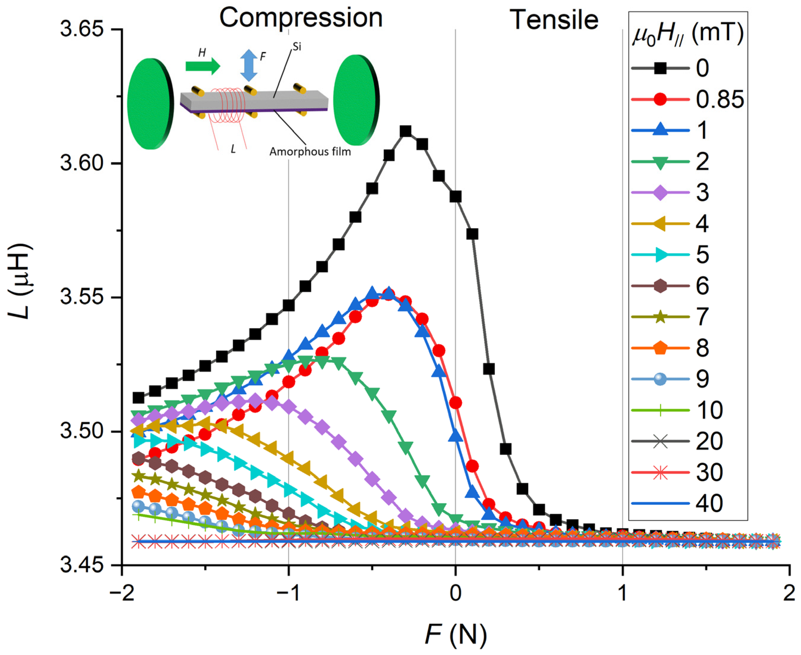
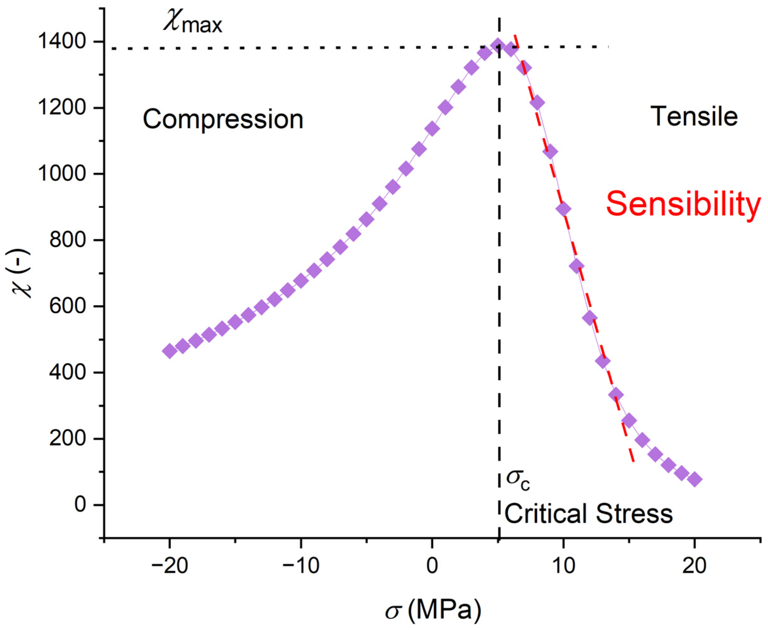
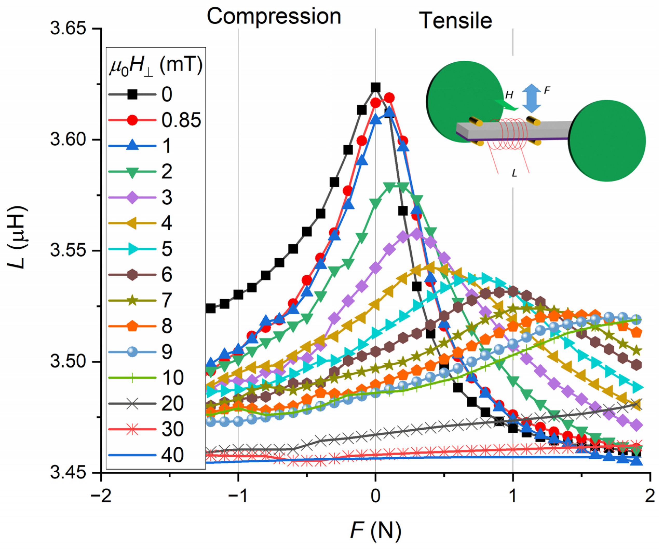
3. Experimental Results
4. Modeling
5. Calculated Results of the Model
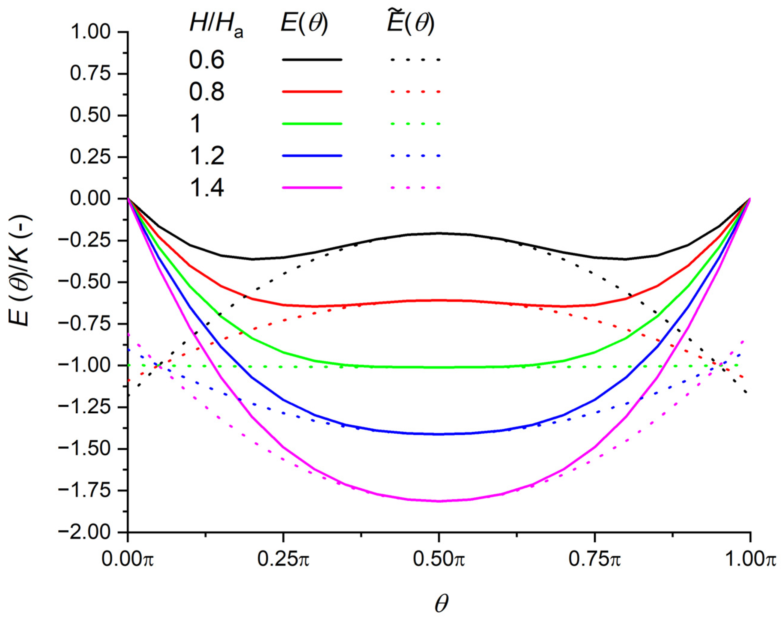
5.1. Without Magnetostriction
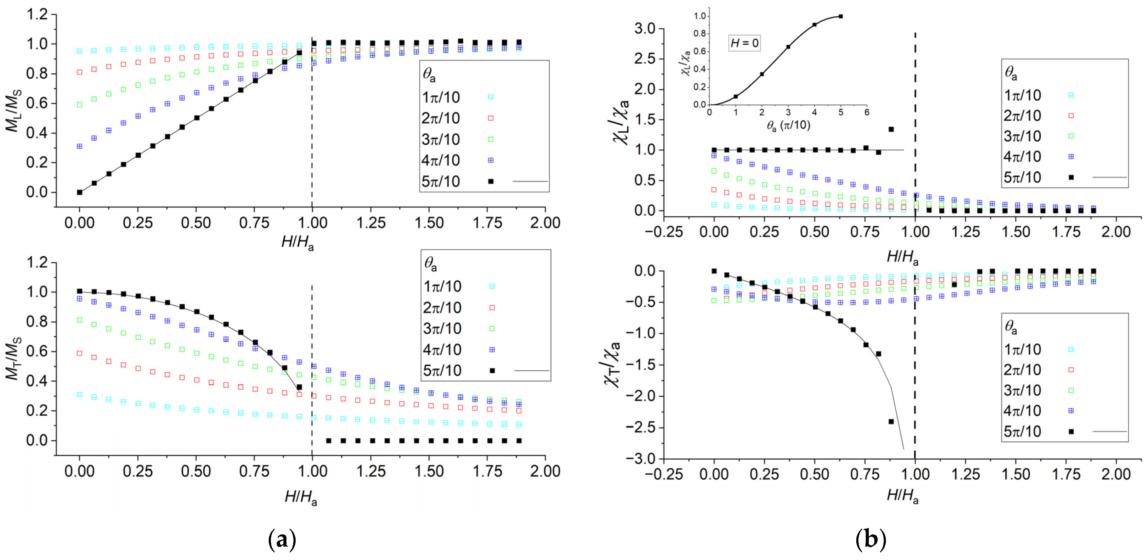
5.2. With Magnetostriction
5.2.1. No External Field
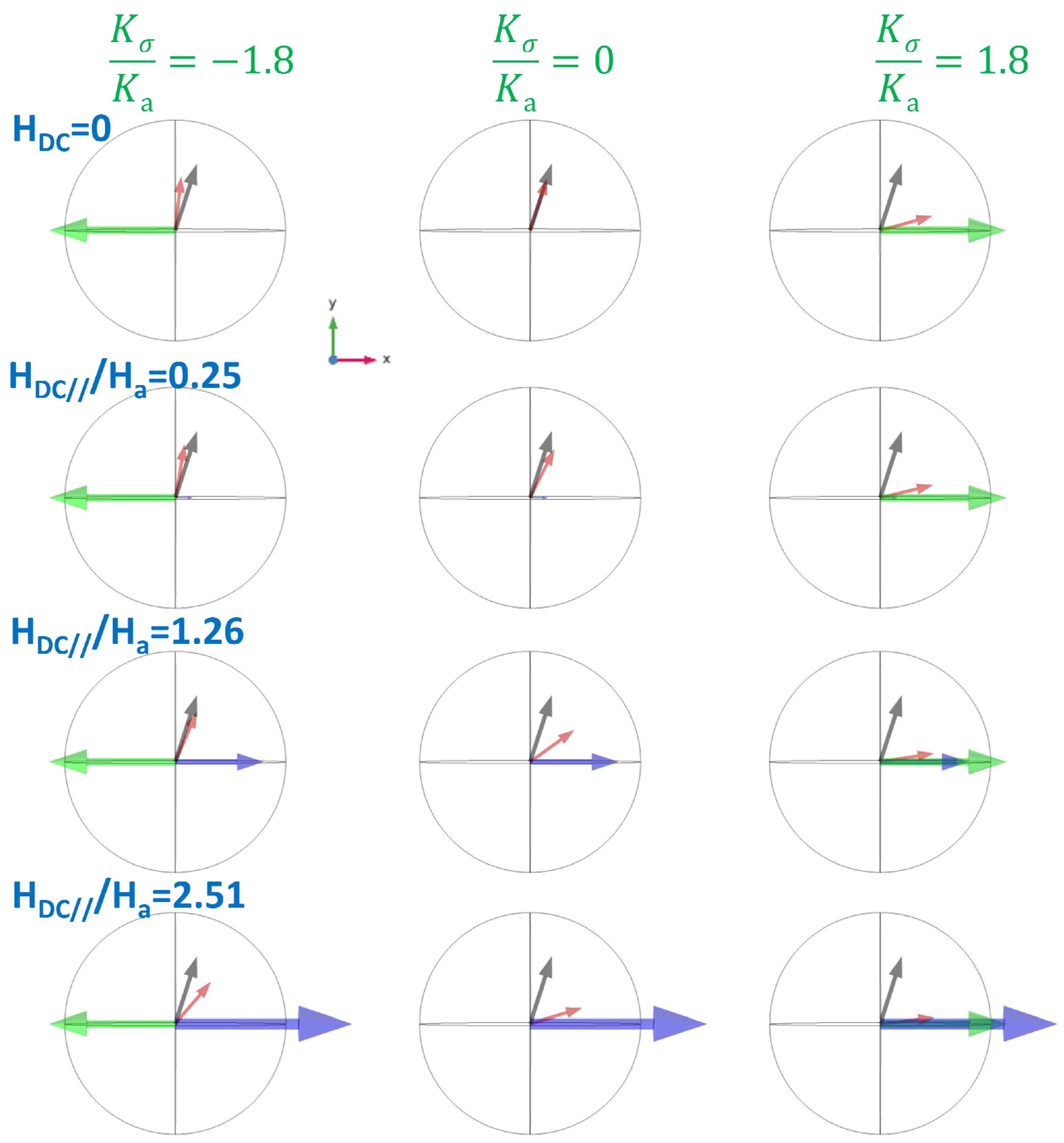
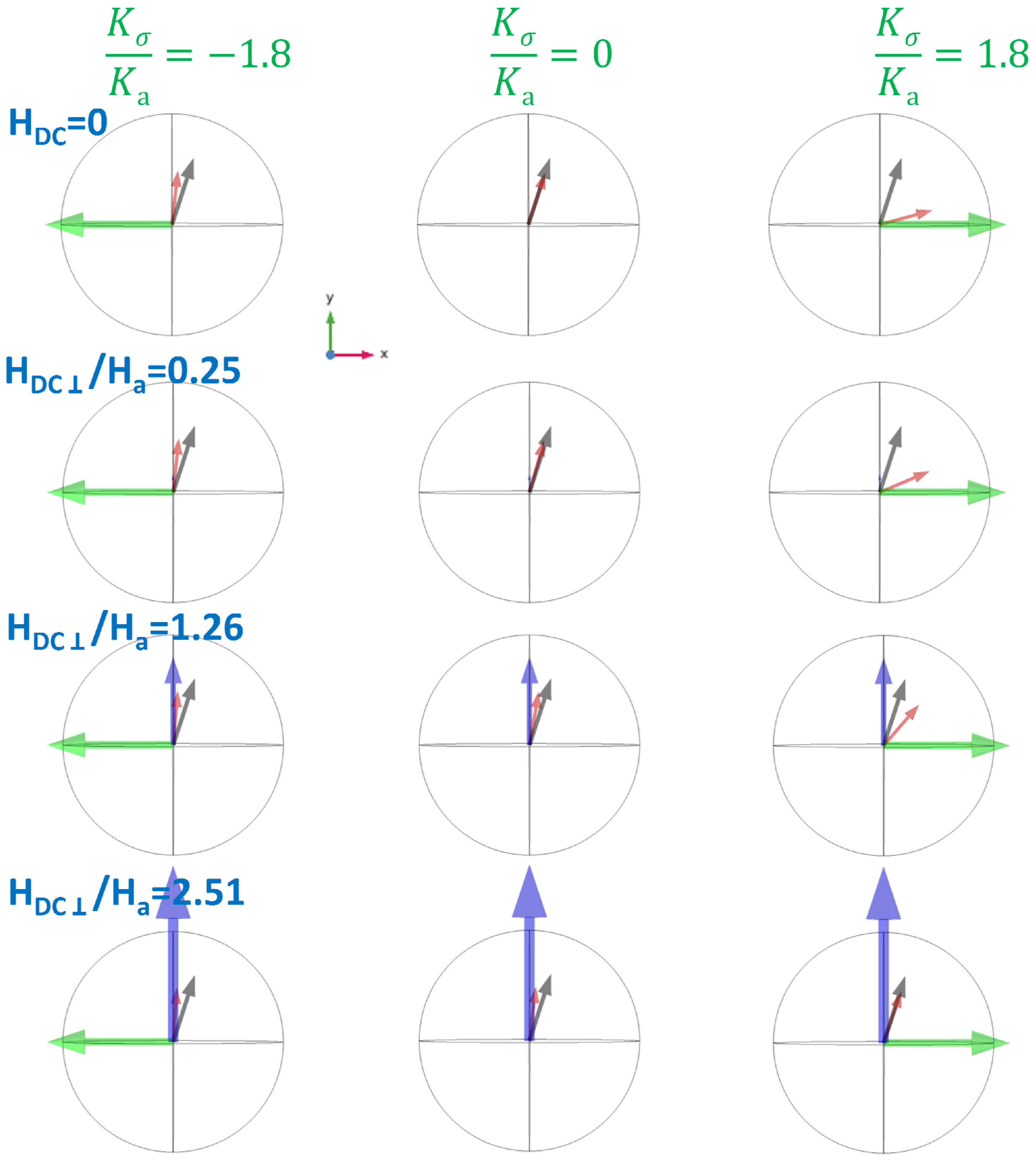
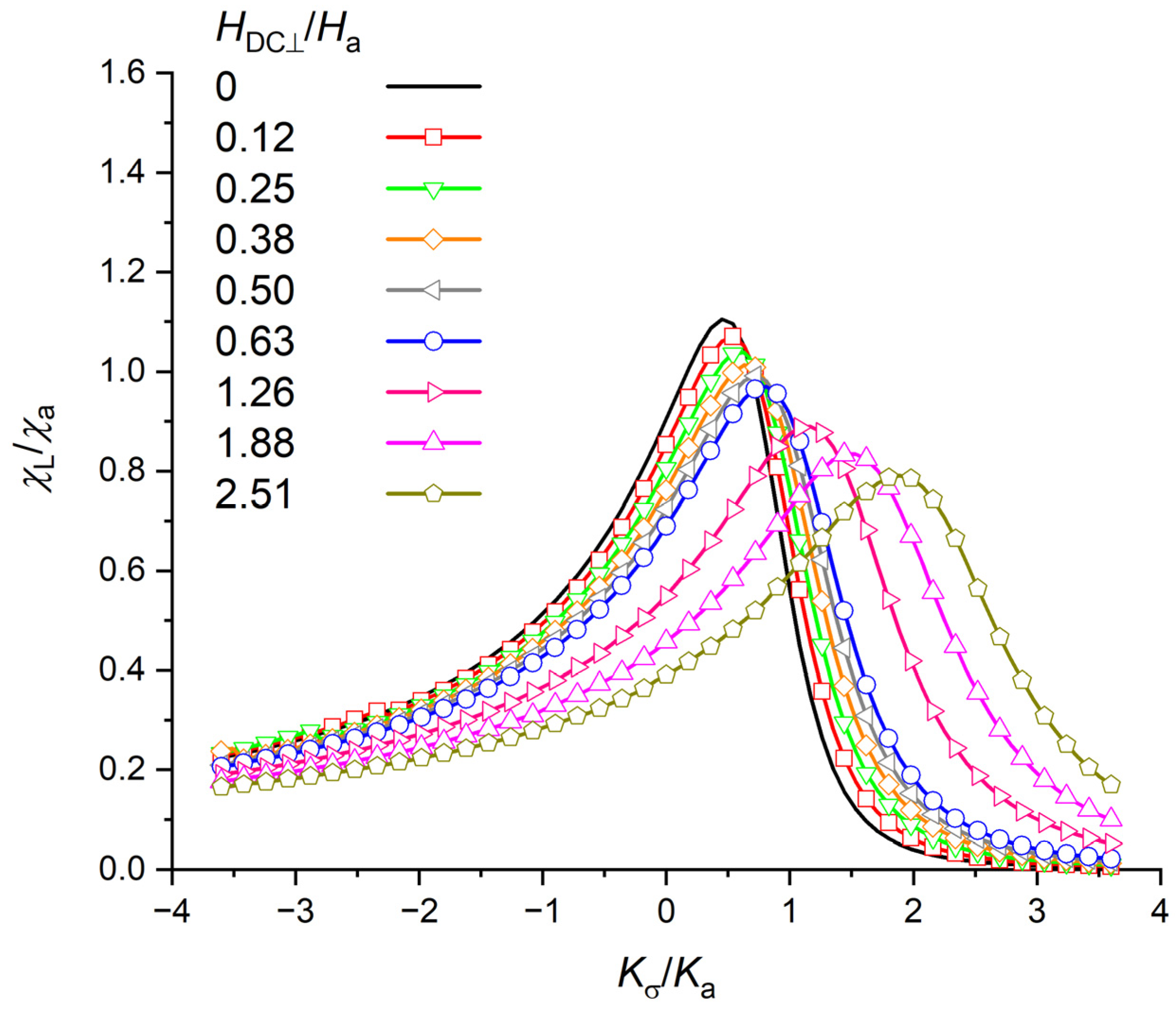
5.2.2. With External Field
6. Conclusions
Author Contributions
Funding
Institutional Review Board Statement
Informed Consent Statement
Data Availability Statement
Conflicts of Interest
Appendix A
Appendix B
Appendix C

References
- Khan, M.A.; Sun, J.; Li, B.; Przybysz, A.; Kosel, J. Magnetic sensors-A review and recent technologies. Eng. Res. Express 2021, 3, 022005. [Google Scholar] [CrossRef]
- Wheeler, H.A. Formulas for the skin-effect. Proc. IRE 1942, 30, 412–424. [Google Scholar] [CrossRef]
- Garcia, D.A.; Munoz, J.L.; Kurlyandskaya, G.; Vasquez, M.; Ali, M.; Gibbs, M.R.J. Induced anisotropy, magnetic domain structure and magnetoimpedance effect in CoFeB amorphous thin films. J. Magn. Magn. Mater. 1999, 191, 339–344. [Google Scholar] [CrossRef]
- Panina, L.V.; Mohri, K. MagnetoImpedance in Multilayer films. Sens. Actuators 2000, 81, 71–77. [Google Scholar] [CrossRef]
- Fosalau, C.; Damian, C.; Zet, C. A high performance strain gage based on the stress impedance effect in magnetic amorphous wire. Sens. Actuators A Phys. 2013, 191, 105–110. [Google Scholar] [CrossRef]
- Hashi, S.; Sora, D.; Ishiyama, K. strain and vibration sensor based on inverse magnetostriction of amorphous magnetostrictive films. IEEE Magn. Lett. 2019, 10, 8110604. [Google Scholar] [CrossRef]
- Froemel, J.; Akita, S.; Tanaka, S. Simple Device to Measure Pressure Using the Stress Impedance Effect of Amorphous Soft Magnetic Thin Layer. Micromachines 2020, 11, 649. [Google Scholar] [CrossRef]
- Blanco, J.M.; Zhokov, A.P.; Gonzalez, J. Torsional stress impedance and magneto-impedance in (Co0.95Fe0.05)72.5Si12.5B15 amorphous wire with helical induced anisotropy. J. Phys. D Appl. Phys. 1999, 32, 3140–3145. [Google Scholar] [CrossRef]
- Shen, L.P.; Uchimiya, T.; Mohri, K.; Kita, E.; Bushida, K. Sensitive stress-impedance micro sensor using amorphous magnetostrictive wire. IEEE Trans. Magn. 1997, 33, 3355–3357. [Google Scholar] [CrossRef]
- Mohri, K.; Uchimiya, T.; Shen, L.P.; Cai, C.M.; Panina, L.V.; Honkura, Y.; Yamamoto, M. Amorphous wire and CMOS IC-based sensitive micromagnetic sensors utilizing magnetoimpedance (MI) and stress-impedance (SI) effects. IEEE Trans. Magn. 2002, 38, 3063–3068. [Google Scholar] [CrossRef]
- Tejedor, M.; Hernando, B.; Sanchez, M.; Prida, V.; Vasquez, M. Magneto-impedance effect in amorphous ribbons for stress sensor applications. Sens. Actuators A Phys. 2000, 81, 98–101. [Google Scholar] [CrossRef]
- Garcia-Arribas, A.; Combarro, L.; Goiriena-Goikoetxea, M.; Kurlyandskaya, G.V.; Svalov, A.V.; Fernandez, E.; Orue, L.; Feuchtwanger, J. Thin-film Magnetoimpedance Structures onto Flexible Substrates as Deformation Sensors. IEEE Trans. Magn. 2017, 53, 2000605. [Google Scholar] [CrossRef]
- Suwa, Y.; Agatsuma, S.; Hashi, S.; Ishiyama, K. Study on impedance change of strain sensor using magnetostrictive film. J. Magn. Soc. Jpn. 2010, 34, 342–346. [Google Scholar] [CrossRef]
- Chen, J.A.; Ding, W.; Zhou, Y.; Cao, Y.; Zhou, Z.M.; Zhang, Z.M. Stress-Impedance effects in sandwiched FeCuNbCrSiB/Cu/FeCuNbCrSiB films. Mater. Lett. 2006, 60, 2554–2557. [Google Scholar] [CrossRef]
- Vincent; Rodriguez, M.; Leong, Z.; Morley, N.A. Design and Development of Magnetostrictive Actuators and Sensors for Structural Health Monitoring. Sensors 2020, 20, 711. [Google Scholar] [CrossRef] [PubMed]
- Froemel, J.; Diguet, G.; Muroyama, M. Micromechanical Force Sensor Using the Stress–Impedance Effect of Soft Magnetic FeCuNbSiB. Sensors 2021, 21, 7578. [Google Scholar] [CrossRef]
- Kurita, H.; Diguet, G.; Froemel, J.; Narita, F. Stress sensor performance of sputtering Fe-Si-B alloy thin coating under tensile and bending loads. Sens. Actuators A Phys. 2022, 343, 113652. [Google Scholar] [CrossRef]
- Usov, N.A.; Antonov, N.A.; Lagar’kov, A.N. Theory of giant magneto-impedance effect in amorphous wires with different types of magnetic anisotropy. J. Magn. Magn. Mater. 1998, 185, 159–173. [Google Scholar] [CrossRef]
- Machado, F.L.A.; Rezende, S.M. A theoretical model for the giant magnetoimpendace in ribbons of amorphous soft-ferromagnetic alloys. J. Appl. Phys. 1996, 79, 6558. [Google Scholar] [CrossRef]
- Jin, F.; Li, J.; Zhou, L.; Peng, J.; Chen, H. Simulation of Giant Magnetic Impedance effect in Co-based Amorphous films with demagnetizing field. IEEE Trans. Magn. 2015, 51, 7100404. [Google Scholar] [CrossRef]
- Chen, H.; Britel, M.R.; Zhukova, V.; Zhukov, A.; Dominguez, L.; Chizik, A.B.; Blanco, J.M.; Gonzalez, J. Influence of AC magnetic field amplitude on the surface magnetoimpedance tensor in amorphous wire with helical magnetic anisotropy. IEEE Trans. Magn. 2004, 40, 3368–3377. [Google Scholar] [CrossRef]
- Kraus, L. Theory of giant magneto-impedance in the planar conductor with uniaxial magnetic anisotropy. J. Magn. Magn. Mater. 1999, 195, 764–778. [Google Scholar] [CrossRef]
- Peng, B.; Zhang, W.L.; Zhang, W.X.; Jiang, H.C.; Yang, S.A. Simulation of stress impedance effect in magnetoelastic films. J. Magn. Magn. Mater. 2005, 288, 326–330. [Google Scholar] [CrossRef]
- Sartorelli, M.L.; Knobel, M. Giant magneto-impedance and its relaxation in Co-Fe-Si-B amorphous ribbons. Appl. Phys. Lett. 1997, 71, 2208. [Google Scholar] [CrossRef]
- Spano, M.L.; Hathaway, K.B.; Savage, H.T. Magnetostriction and magnetic anisotropy of field annealed Metglas 2605 alloys via M-H loop measurements under stress. J. Appl. Phys. 1982, 53, 2667. [Google Scholar] [CrossRef]
- Livingston, J. Magnetomechanical properties of amorphous metals. Phys. Status Solidi A 1982, 70, 591–596. [Google Scholar] [CrossRef]
- He, D.F.; Shiwa, M. A magnetic sensor with amorphous wire. Sensors 2014, 14, 10644–10649. [Google Scholar] [CrossRef]
- Mendoza Zelis, P. Magnetostrictive bimagnetic trilayer ribbons for temperature sensing. J. Appl. Phys. 2006, 101, 034507. [Google Scholar] [CrossRef]
- Shin, K.H.; Inoue, M.; Arai, K.I. Elastically coupled magneto-electric elements with highly magnetostrictive amorphous films and PZT subtrates. Smart Mater. Struct. 2000, 9, 357–361. [Google Scholar] [CrossRef]
- Ludwig, A.; Frommberger, M.; Tewes, M.; Quandt, E. High-frequency magnetoelastic multilayer thin films and applications. IEEE Trans. Magn. 2003, 39, 3062. [Google Scholar] [CrossRef]
- Appino, C.; Fiorillo, F.; Maraner, A. initial susceptibility versus applied stress in amorphous alloys with positive and negative magnetostriction. IEEE Trans. Magn. 1993, 29, 3469–3471. [Google Scholar] [CrossRef]
- Kubo, Y.; Hashi, S.; Yokoi, H.; Arai, K.; Ishiyama, K. Development of strain and vibration sensor using magnetostriction of magnetic thin film. IEEE Trans. Sens. Micromach. 2018, 138, 153–158. (In Japanese) [Google Scholar] [CrossRef]
- Ding, Q.; Li, J.; Zhang, R.; He, A.; Dong, Y.; Sun, Y.; Zheng, J.; Li, X.; Liu, X. Effect of transverse magnetic field annealing on the magnetic properties and microstructure of FeSiBNbCuP nanocrystalline alloys. J. Magn. Magn. Mater. 2022, 560, 169628. [Google Scholar] [CrossRef]
- Cullity, B.D.; Graham, C.D. Magnetic anisotropy. In Introduction to Magnetic Materials, 2nd ed.; John Wiley and Sons Inc.: Hoboken, NJ, USA, 2008. [Google Scholar]


| Quantity | Direction |
|---|---|
| DC field H | Field H// (x-direction) or Field HꞱ (y-direction) |
| AC field hac | x-direction |
| Stress σ | x-direction |
| Anisotropy axis | At angle θa to x-direction |
| Magnetization M | Longitudinal ML (x-direction) or Transverse MT (y-direction) |
| Quantity | Linear Slope Coefficient | Decay Coefficient |
|---|---|---|
| [σc(H//) − σc(H//= 0)]/σc(H// = 0) | −1.72 (-) 1 | - |
| [σc(HꞱ) − σc(HꞱ = 0)]/σc(HꞱ = 0) | 1.27 (-) 1 | - |
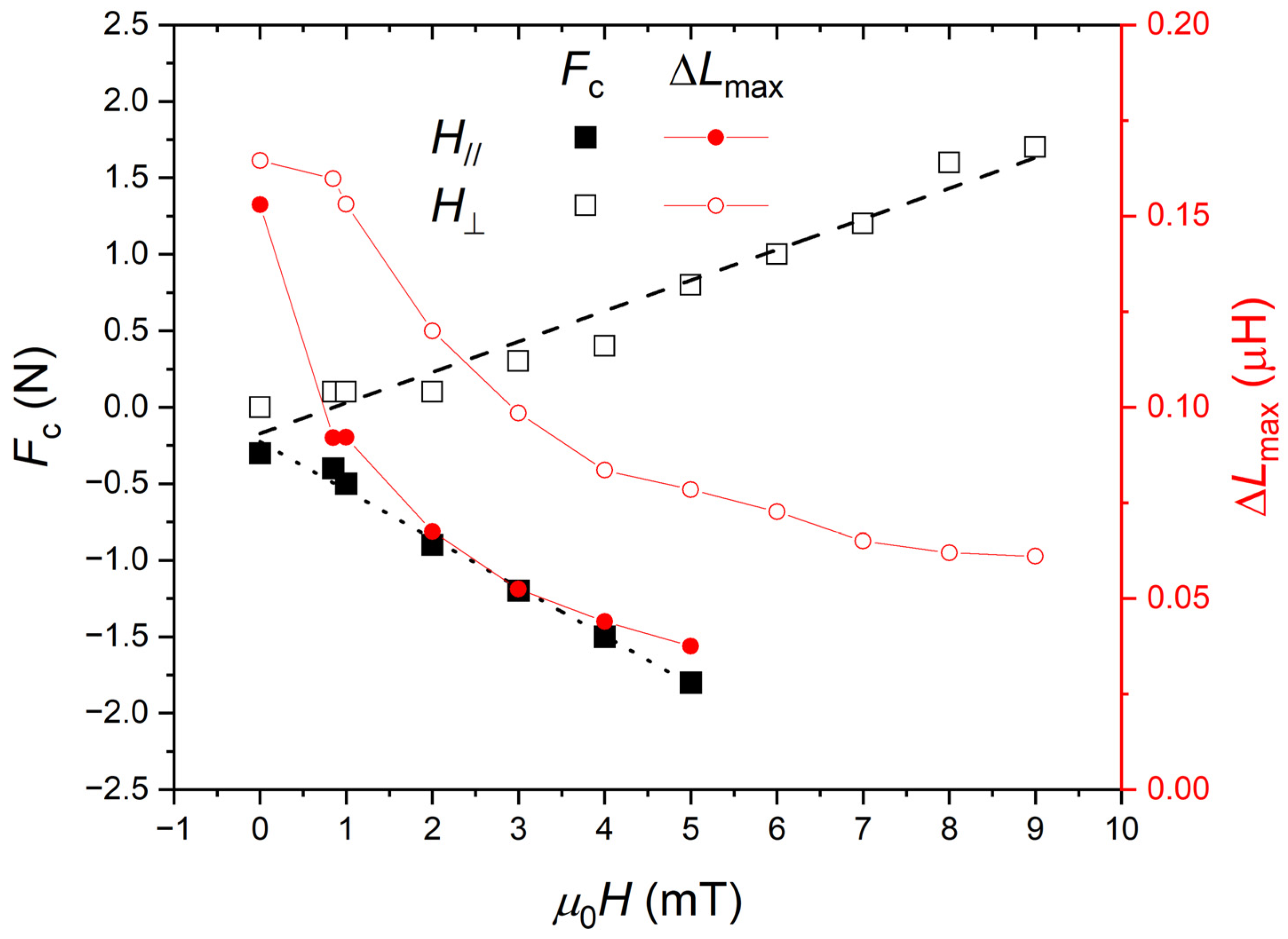
| [Fc(H//) − Fc(H// = 0)] | −0.29 N/(mT) 2 | - |
| [Fc(HꞱ) − Fc(HꞱ = 0)] | 0.16 N/(mT) 2 | - |
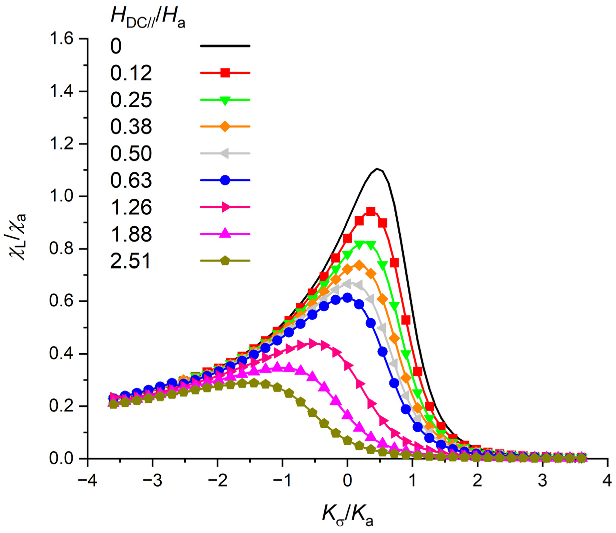
| χL(H//)/χa | - | 0.68 (-) 1 |
| χL(HꞱ)/χa | - | 1.48 (-) 1 |
| ΔLmax(H//) | - | 1.32 (mT−1) 2 |
| ΔLmax(HꞱ) | - | 3.67 (mT−1) 2 |
Publisher’s Note: MDPI stays neutral with regard to jurisdictional claims in published maps and institutional affiliations. |
© 2022 by the authors. Licensee MDPI, Basel, Switzerland. This article is an open access article distributed under the terms and conditions of the Creative Commons Attribution (CC BY) license (https://creativecommons.org/licenses/by/4.0/).
Share and Cite
Diguet, G.; Froemel, J.; Kurita, H.; Narita, F.; Makabe, K.; Ohtaka, K. Magneto Elasticity Modeling for Stress Sensors. Magnetism 2022, 2, 288-305. https://doi.org/10.3390/magnetism2030021
Diguet G, Froemel J, Kurita H, Narita F, Makabe K, Ohtaka K. Magneto Elasticity Modeling for Stress Sensors. Magnetism. 2022; 2(3):288-305. https://doi.org/10.3390/magnetism2030021
Chicago/Turabian StyleDiguet, Gildas, Joerg Froemel, Hiroki Kurita, Fumio Narita, Kei Makabe, and Koichi Ohtaka. 2022. "Magneto Elasticity Modeling for Stress Sensors" Magnetism 2, no. 3: 288-305. https://doi.org/10.3390/magnetism2030021
APA StyleDiguet, G., Froemel, J., Kurita, H., Narita, F., Makabe, K., & Ohtaka, K. (2022). Magneto Elasticity Modeling for Stress Sensors. Magnetism, 2(3), 288-305. https://doi.org/10.3390/magnetism2030021