Electromagnetic Tracking of Elongated Sensors for Endoscopic Navigation

Abstract

As the prevalence of image-guided interventions increases, electromagnetic tracking (EMT) systems play an important role in modern patient care, as they enable real-time instrument positioning and navigation inside the human body without line-of-sight restrictions. Miniature-size inductive coils are the gold standard in clinical settings, as they provide accurate, passive sensing of the magnetic field. To compensate for their small dimensions, such sensors are designed with an elongated shape, where the coil length is usually 10 to 20 times larger than the diameter. In this article, the benefits of a field model based on the magnetic scalar potential formulation are demonstrated for EMT applications where elongated tracking sensors are used. The novel method resolves the single-point approximation error when the coil length is not negligible, and demonstrates improvements in terms of speed and storage requirements. A detailed analysis is proposed where alternative formulations of the magnetic model used in the tracking algorithm are compared. Although this work does not resolve any substantial limits of EMT used in a clinical environment, which are mainly caused by the presence of magnetic distortions, the proposed method is an improvement over existing EMT systems because it enables more accurate and faster tracking. The method might facilitate the use of longer tracking sensor coils which can achieve high sensitivities without the requirement of a magnetic core. In the envisioned application, such coils may be wound around flexible instruments, such as endoscopes or catheters.

1. Introduction

Magnetic tracking, or electromagnetic tracking (EMT), enables instrument positioning and navigation during image-guided interventions [1,2]. As opposed to optical tracking, the technology allows to track objects without a line of sight, and therefore it finds applications in minimally invasive surgery to localise instruments inside the human body [3]. Examples of clinical procedures that exploit EMT include non-fluoroscopic catheter tracking [4,5], orthopaedic surgery [6], robotic bronchoscopy [7], and percutaneous urology [8]. The reader is directed to [9] for a recent review on the use of electromagnetic tracking and positioning in endoscopy.

In the most common EMT architecture, an external field generator, comprising multiple emitter coils, generates a signal, and a small magnetic sensor attached to the target instrument is used as a marker. Knowledge of the magnetic field in the volume of interest allows finding the position and orientation of every sensor, as a reverse problem from the received signal [10,11].

Magnetic sensors used in endoscopy applications are generally induction pick-up coils, which are passive by nature and therefore reduce risk in the event of a malfunctioning medical device. Such coils can be manufactured to miniature sizes of less than 0.5 mm in diameter [12], and they provide higher sensitivities in the presence of AC-excitation magnetic fields [13,14]. However, to guarantee human safety, the EMT systems used in clinical settings have limited magnetic field amplitudes and, in order to meet the sensitivity requirements, the sensor coils must be designed with an elongated shape, in the centimetre scale. This might introduce positioning errors of the tracked sensor when the coil’s length cannot be ignored if compared to the field spatial variation.

An accurate understanding of the real magnetic field is essential for sub-millimetre sensor tracking. For this reason, field generator coils are usually designed to imitate simple analytical field models, such as the ideal magnetic dipole [15], current filaments [16], or current sheets [17]. The field spatial variation also plays an important role in increasing the resolution and precision of the tracking, as well as ensuring fast and global convergence if the gradient is monotonic [18]. To overcome the limits imposed by an analytical model, and/or to take into account the presence of static magnetic distortions, such as passive shields or nearby electronics, data-driven field models can be obtained from volume characterisation where the magnetic field values are stored in a look-up table [18,19].

In this article, we introduce an alternative formulation for the field model, which is based on the magnetic scalar potential and shows improvements in terms of speed and storage requirements, and can inherently take into account the length of the inductive sensor coil. This work is the counterpart of the method previously published in [20], where the finite dimension of large-area planar sensor coils is resolved using a magnetic vector potential expression to reduce EMT errors.

To implement and validate the novel model, the open-source platform Anser EMT was used [21]. The system provides an open framework to assist research in the EMT field [22] and a modular software environment [23,24], which allowed access to the magnetic field model and tracking algorithm for the experiments presented in this work.

The article is structured as follows. Section 2 provides the theoretical background and presents the derivation of an analytical model for the magnetic scalar potential of filament-based spiral coils, such as those used in the Anser EMT field generator. The experiments performed in this work are introduced in Section 3. In particular, storage requirements and interpolation performance are analysed for the existing field model and the novel formulation compared. Then, the speed and accuracy of the two models are evaluated by means of simulated and real tracking tests. Finally, a tracking method is proposed to localise flexible sensor coils of several centimetres in length. The experiments’ results are outlined in Section 4 and the main findings are commented upon in Section 5. Section 6 concludes the article.

2. Magnetic Model of Elongated Sensors

Inductive magnetic sensors work on the principle of magnetic induction, described by Faraday’s law, which states that the electromotive force, V, on a static loop is equal to the negative of the time derivative of the magnetic flux, $\mathrm{\Phi }$, crossing that loop, as per Equation (1):

$$V=-\frac{\partial \mathrm{\Phi }}{\mathrm{\partial }t}.$$

(1)

The magnetic flux $\mathrm{\Phi }$ is calculated as the surface integral of the magnetic flux density B over the cross-sectional coil area, $A_c$. For small-diameter coils, such as those studied in this work, B can be considered to be constant across the loop and the magnetic flux is given by:

$$\mathrm{\Phi }=\mathbf{B}·\mathbf{n}{A}_c,$$

(2)

where n is the unit vector perpendicular to $A_c$.

An inductive coil comprises a number N of consecutive turns, each of them experiencing a magnetic flux calculated according to Equation (2). If the coil is long relative to the spatial variation of B, in other words if it cannot be assumed for B to be constant or linearly varying across the sensor length, the induced voltage must be calculated by the line integral of B along the coil:

$$\mathrm{\Phi }=A_c{\int }_A^B\mathbf{B}·\mathbf{n}n\left(l\right)dl=A_c\frac{N}{L}{\int }_A^B\mathbf{B}·\mathbf{n}dl=A_{c}N\langle \mathbf{B}\rangle ·\mathbf{n},$$

(3)

where $n=N/L$ is the turn density, which is assumed constant, L is the length of the coil, A and B are the coil end-points, $\langle \mathbf{B}\rangle$ is the average magnetic flux density along the coil, and the unit vector n identifies the orientation and is constant for a rigid sensor.

Electromagnetic fields are described by Maxwell’s equations [25]. In the magnetostatics approximation, the equations for the magnetic field are:

$$\begin{array}{cc}\hfill & \nabla ·\mathbf{B}=0,\hfill \end{array}$$

(4)

$$\begin{array}{cc}\hfill & \nabla \times \mathbf{H}=\mathbf{J},\hfill \end{array}$$

(5)

with $\mathbf{B}=\mathsf{\mu }\mathbf{H}$, where $\mu$ is the magnetic permeability of the medium, $\mathbf{H}$ is the magnetic field intensity and $\mathbf{J}$ is the current density.

Equation (5) is also known as Ampere’s law and, in current-free volumes when $\mathbf{J}=0$, the magnetic field is curl-free: $\nabla \times \mathbf{H}=0$. Therefore, in regions of the space where there is no electric current, the magnetic field vector can be expressed as the gradient of a magnetic scalar potential, $\psi$:

$$\mathbf{H}=-\nabla \psi .$$

(6)

Because, for the frequencies of interest, biological tissues have the same magnetic permeability as free space, ${\mu }_0$, the integral of Equation (3) can be expanded using Equation (6):

$${\int }_A^B\mathbf{B}·\mathbf{n}dl=-{\mu }_0{\int }_A^B\nabla \psi \times \mathbf{n}dl=-{\mu }_0{\int }_A^B\frac{\partial \psi }{\partial l}dl=-{\mu }_0{\int }_{{\psi }_A}^{{\psi }_B}d\psi ={\mu }_0({\psi }_A-{\psi }_B).$$

(7)

when the tracking of elongated sensors is involved, Equation (3) is usually resolved by evaluating $\mathbf{B}$ at the sensor midpoint. If this introduces unacceptable position errors, $\langle \mathbf{B}\rangle$ may be approximated using an n-point quadrature rule [26,27] at the cost of speed. Therefore, it may be computationally more convenient to calculate the magnetic flux from Equation (8), obtained after substituting Equation (7) in Equation (3):

$$\mathrm{\Phi }=\frac{{\mu }_0{A}_{c}N}{L}({\psi }_A-{\psi }_B).$$

(8)

Equations (3) and (8) will be the basis for the two analytical magnetic flux models used in this work.

2.1. Biot–Savart Model of the Anser EMT Field Generator

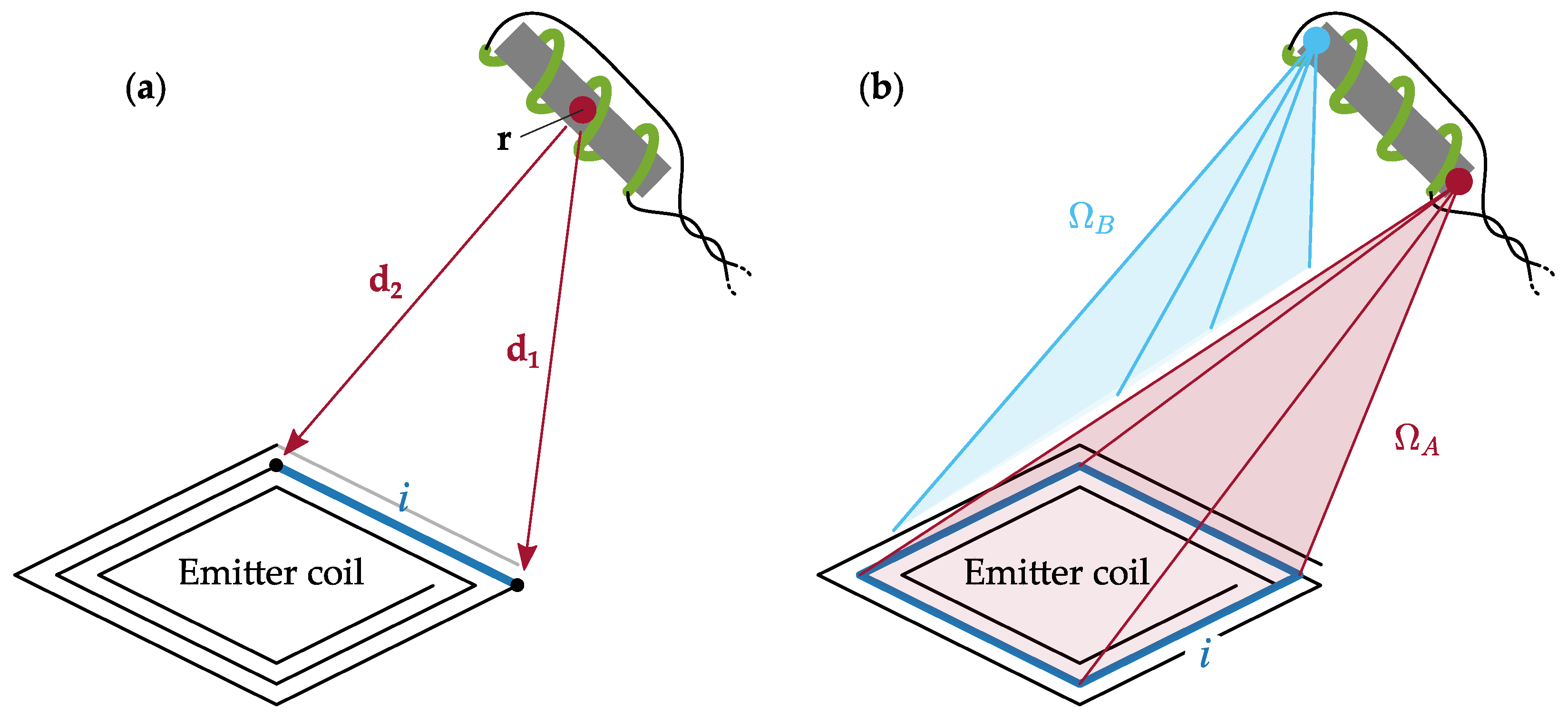
The open-hardware Anser EMT system [21] was used in this work. The field generator is a two-layer printed circuit board comprising eight equal planar emitter coils. Each emitter coil has a square shape with an external edge of 70 mm and can be modelled as a combination of 100 straight current filaments [28].

At the evaluation point identified by the position vector $\mathbf{r}$, the magnetic field $\mathbf{H}\left(\mathbf{r}\right)$ generated by each emitter coil can be calculated using the Biot–Savart law [29]:

$$\mathbf{H}\left(\mathbf{r}\right)=\frac{I}{4\pi }{\int }_{\Gamma }\frac{\mathbf{t}\times \mathbf{r}}{R^3}d\Gamma ,$$

(9)

where I is the electric current in the coil, $\Gamma$ is the current path along the coil winding, $\mathbf{t}$ is the tangential unit vector and $R=\left|\mathbf{r}\right|$.

As mentioned above, $\Gamma$ can be decomposed into straight wires, each of which in Equation (9) can be integrated in closed form, as expressed by Equation (10) [30]:

$${\mathbf{H}}_{\mathbf{i}}\left(\mathbf{r}\right)=\frac{I}{4\pi }\left(\frac{{\mathbf{d}}_{\mathbf{2}}\times {\mathbf{d}}_{\mathbf{12}}}{\parallel {\mathbf{d}}_{\mathbf{2}}\times {\mathbf{d}}_{\mathbf{12}}{\parallel }^2}\right)\left(\frac{{\mathbf{d}}_{\mathbf{12}}·{\mathbf{d}}_{\mathbf{2}}}{\parallel {\mathbf{d}}_{\mathbf{2}}\parallel }-\frac{{\mathbf{d}}_{\mathbf{12}}·{\mathbf{d}}_{\mathbf{1}}}{\parallel {\mathbf{d}}_{\mathbf{1}}\parallel }\right),$$

(10)

where ${\mathbf{d}}_{\mathbf{1}}$ and ${\mathbf{d}}_{\mathbf{2}}$ are the vectors from the evaluation point, $\mathbf{r}$, to the straight filament’s end-points and ${\mathbf{d}}_{\mathbf{12}}={\mathbf{d}}_{\mathbf{2}}-{\mathbf{d}}_{\mathbf{1}}$, as defined in Figure 1a.

For every emitter coil in the field generator, the total magnetic field is given by the superposition of the 100 straight wires that compose the coil:

$$\mathbf{H}\left(\mathbf{r}\right)=\sum _{i=1}^{100}{\mathbf{H}}_{\mathbf{i}}\left(\mathbf{r}\right),$$

(11)

where each contribution ${\mathbf{H}}_{\mathbf{i}}\left(\mathbf{r}\right)$ is calculated as per Equation (10).

Finally, for a tracking sensor at position r and oriented along n, the magnetic flux crossing the sensor winding is given by substituting Equation (11) in Equation (3):

$$\mathrm{\Phi }(\mathbf{r},\mathbf{n})={\mu }_0{A}_{c}N\mathbf{H}\left(\mathbf{r}\right)·\mathbf{n},$$

(12)

which has to be calculated for every emitter coil in the field generator.

According to this model, the magnetic sensor is approximated as a single point located at r and $\mathbf{H}\left(\mathbf{r}\right)$ represents the average magnetic field along the coil. In the remainder of this article, we refer to Equation (12) as the single-point model of the field generator.

2.2. Scalar Potential Formulation of the Field Generator Model

In this section, a scalar potential formulation is obtained for the magnetic field of the Anser EMT system.

As can be verified, the magnetic field given by the Biot–Savart law, Equation (9), satisfies Ampere’s Law, Equation (5) only if the divergence of the current density $\mathbf{J}$ is zero everywhere in the space [31], as is the case for steady currents in closed loops.

A finite segment of wire has a source of current at one end of the wire and a sink of current at the other. Therefore, the current is not divergence-free and ${\mathbf{H}}_{\mathbf{i}}\left(\mathbf{r}\right)$ of Equation (10) does not satisfy Ampere’s law. In particular, the magnetic field due to each individual wire composing the emitter coils is not curl-free, even at points where there is no current, and it cannot have a scalar potential formulation.

For this reason, it is not possible to express the scalar potential of $\mathbf{H}\left(\mathbf{r}\right)$ as a sum of contributions due to individual wire segments, as is done in Equation (11), but the closed current path of the emitter coil must be considered in full.

A scalar potential for the field generated by the current I in the closed loop $\Gamma$ is given by Equation (13):

$$\psi \left(\mathbf{r}\right)=-\frac{I}{4\pi }\Omega ,$$

(13)

where $\Omega$ is the solid angle for the area enclosed by the loop $\mathrm{\Gamma }$, subtended at point $\mathbf{r}$ [32]. Once more, it is clear that the loop $\mathrm{\Gamma }$ must be closed because it is defined as the boundary of a surface.

The solid angle bounded by a rectangular spiral, such as the current path formed by the emitter coils considered in this work, can be calculated as detailed in Appendix A. Alternatively, it is possible to approximate the spiral as a set of concentric squares, as shown in Figure 1b, and to calculate the total solid angle enclosed by each emitter coil as the sum of the solid angles covered by rectangular plates [33].

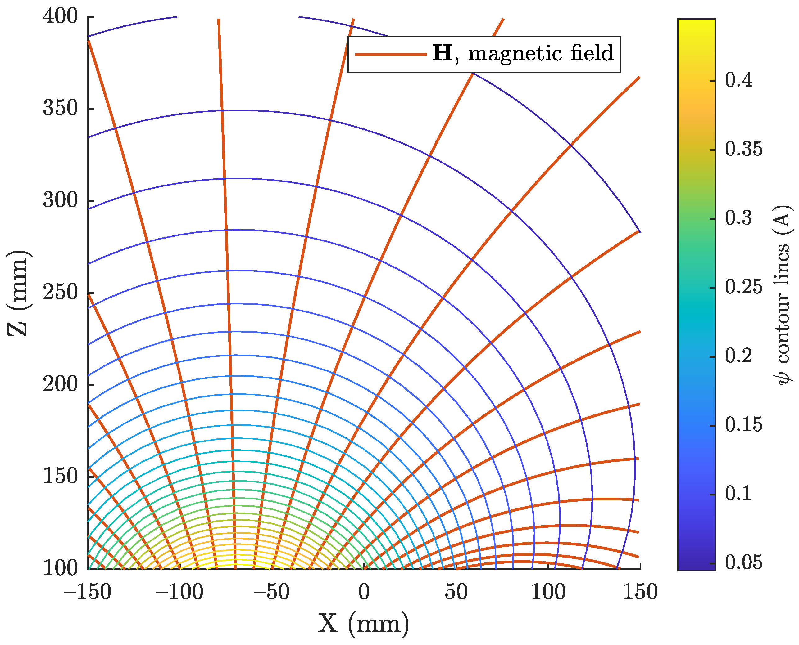
The magnetic field model and the corresponding scalar potential formulation are visualised in Figure 2, for the emitter coil highlighted in Figure 3a, which is coil number 4 as defined in Figure 4. It can be seen that the contour lines of $\psi$ are always perpendicular to the field lines, as expected, considering that the $\mathbf{H}$ field was defined as $-\nabla \psi$.

Finally, for a tracking sensor at position r and oriented along n, the magnetic flux crossing the sensor winding is obtained by substituting Equation (13) into Equation (8):

$$\mathrm{\Phi }(\mathbf{r},\mathbf{n})=\frac{{\mu }_0{A}_{c}N}{L}\left(\psi \left(\mathbf{r}-\mathbf{n}\frac{L}{2}\right)-\psi \left(\mathbf{r}+\mathbf{n}\frac{L}{2}\right)\right),$$

(14)

which has to be calculated for every emitter coil in the field generator.

According to this model, the total length of the magnetic sensor is taken into account. In the remainder of this article, we refer to Equation (14) as the full-length model of the field generator.

3. Materials and Methods

The full-length model introduced in this article, based on the magnetic scalar potential formulation, was evaluated in terms of speed and accuracy and compared with the single-point model currently used by the Anser EMT system. In the two cases, interpolation performance was tested for different grid densities and a criterion to select the optimal grid spacing is presented. All models were tested on simulated and real electromagnetic tracking experiments.Finally, methods for the electromagnetic tracking of a long flexible sensor were exposed and tested by means of a simulation.

3.1. Performance Metrics

In this study, the following metrics were used to compare the different magnetic field predictions of the models analysed and the corresponding error in the position tracking of the electromagnetic sensor.

We define $\mathbf{x}\in {\mathbb{R}}^{8M\times 1}$ and $\mathbf{y}\in {\mathbb{R}}^{8M\times 1}$ as the vectors comprising the magnetic field predictions and reference values, respectively, for the eight emitter coils, where M is the total number of observations.

The average field error was defined as the Normalised Mean Absolute Error (NMAE), where the range of the observations was used as the normalisation parameter:

$$\mathrm{NMAE}(\mathbf{x},\mathbf{y})=\frac{1}{8M}\sum _{i=1}^{8M}\left|x_i-y_i\right|/\left(\underset{i}{max}\mathbf{y}-\underset{i}{min}\mathbf{y}\right).$$

(15)

It can be noticed that, since the eight emitter coils are equal, the corresponding magnetic models only differ by a roto-translation, and averaging between all the test positions is effectively equivalent to considering $M\times 8$ random points for the field model of a singular emitter coil.

Since the final aim is to find the position and orientation of the target sensor, it is more informative to calculate the electromagnetic tracking position error associated with the field difference. We define $\mathbf{p}\in {\mathbb{R}}^{5\times 1}$ as the pose vector of the uni-axial elongated sensor:

$$\mathbf{p}=\left[x,y,z,\theta ,\phi \right],$$

(16)

where x, y, and z are the Cartesian coordinates of the sensor position, and $\theta$ and $\phi$ are the angles defining the sensor orientation in spherical coordinates. The flux vector $\mathrm{\Phi }\in {\mathbb{R}}^{8\times 1}$ contains the sensor measurements relative to the eight emitter coils.

If $\tilde{\mathrm{\Phi }}$ is the vector of the perturbed magnetic flux values and $\tilde{\mathbf{p}}$ is the corresponding sensor pose estimation, a Taylor expansion is performed around the reference sensor location:

$$\tilde{\mathrm{\Phi }}\approx \mathrm{\Phi }+{\mathbf{J}}_{\mathbf{p}}·(\tilde{\mathbf{p}}-\mathbf{p}),$$

(17)

where ${\mathbf{J}}_{\mathbf{p}}\in {\mathbb{R}}^{8\times 5}$ is the Jacobian matrix of the flux model calculated in p.

The pose error, $\Delta \mathbf{p}=(\tilde{\mathbf{p}}-\mathbf{p})$, can be estimated from the field difference, $\Delta \Phi =(\tilde{\mathrm{\Phi }}-\mathrm{\Phi })$, by inverting Equation (17):

$$\Delta \mathbf{p}={\mathbf{J}}_{\mathbf{p}}^{+}·\Delta \mathrm{\Phi },$$

(18)

where ${\mathbf{J}}_{\mathbf{p}}^{+}$ is the Moore–Penrose inverse of the matrix ${\mathbf{J}}_{\mathbf{p}}$.

In particular, the position error was calculated at each test point as the Euclidean distance between the predicted and the reference sensor positions, which correspond to the first three elements of $\tilde{\mathbf{p}}$ and p respectively:

$$e=\sqrt{{(\tilde{x}-x)}^2+{(\tilde{y}-y)}^2+{(\tilde{z}-z)}^2}\left[\mathrm{mm}\right].$$

(19)

The total angular displacement was obtained as given by Equation (20), from the two spherical angles errors, $\Delta \theta$ and $\Delta \phi$, which correspond to the last two elements of $\Delta \mathbf{p}$:

$$e=\frac{{180}^{\circ }}{\pi }\sqrt{\Delta {\theta }^2+{sin}^2\left(\theta +\frac{\Delta \theta }{2}\right)\Delta {\phi }^2}.$$

(20)

Average position and orientation errors were expressed as the root mean square error (RMSE) and the mean error (ME), calculated on the number M of observations:

$$\mathrm{RMSE}\left(\mathbf{e}\right)=\sqrt{\frac{1}{M}{\sum }_{i=1}^M{e}_i^2};\mathrm{ME}\left(\mathbf{e}\right)=\frac{1}{M}\sum _{i=1}^M{e}_i,$$

(21)

where $\mathbf{e}$ is the vector with entries $e_i$, which is the position or, alternatively, the orientation error at the test point i.

To give an insight into the error distribution, the median or 50th percentile (PRC50) and the 95th percentile (PRC95) were used.

3.2. Model Interpolation

In order to speed up the tracking algorithm of the EMT system, it is common to pre-evaluate the electromagnetic model at grid points within the region of interest and to store the data in a look-up table (LUT). The values at any point of the volume are given by interpolating between grid points.

The interpolation error was evaluated for the magnetic scalar potential and for the magnetic field vector. In the first case, only one scalar value is stored, while in the second case, the three field components are saved separately. However, the magnetic field is obtained from the scalar potential after the gradient operation, which decreases by one degree the order of the interpolation polynomial. Therefore, even if the storage intake is 1/3 as large for scalar potential when the grid size is not changed, in order to obtain the same level of accuracy it may be required to decrease the spacing between grid-points, which would increase the number of stored values following a cubic power law.

The interpolation performance was evaluated for different grid densities within a $30\times 30\times 30{\mathrm{cm}}^3$ cubic volume placed 10$\mathrm{cm}$ above the field generator. Regular interpolation grids were considered and the same grid spacing was used in the three dimensions.

The LUTs were generated by evaluating and storing the scalar potential, or the three field components respectively, at the grid points, for the eight emitter coils of the field generator.

To calculate the interpolation error, 10,000 positions were randomly selected inside the working volume and the interpolated values were predicted using a tricubic spline interpolation with not-a-knot end conditions. At every point, a random orientation was used to calculate the magnetic fluxes as per Equations (12) and (14), for the two models respectively.

The interpolation error was calculated with respect to the analytical model reference, both for the flux values and for the tracking position, as described in Section 3.1.

For each density of the grid, the size of each LUT was obtained using the whos function in MATLAB (Mathworks, Natick, MA, USA).

3.3. Simulated Tracking Test

For the full-length and the single-point magnetic flux formulations compared in this article, two LUTs were selected which give approximately the same interpolation error and require similar storage space, as will be justified in Section 4.1.

For convenience, in the remainder of the article, we will refer to these tabulated models as LUT FL, for the table storing the magnetic scalar potential, and LUT SP, for the table of the three magnetic field components based on the Biot–Savart law.

The four models, the two analytical and the two LUTs, were compared and the differences were quantified using synthetic data. In this way, it was possible to decouple the sources of error: (1) the physical approximation of the sensor as a single point, which was compared to the new formulation that takes into account the full sensor length, and (2) the numerical approximation due to the cubic spline interpolation.

The same cubic volume used in Section 3.2 was considered. Within this region, 100,000 random positions and orientations were selected for an elongated sensor with a length of 10$\mathrm{mm}$.

The magnetic fluxes NMAE and the tracking position errors were calculated as described in Section 3.1. The error introduced by the single-point approximation was calculated with respect to the full-length model, while the error of each LUT was compared to the respective analytical model.

The speed of the four models was computed as an average on the 100,000 flux evaluations, using the tic-toc function in MATLAB, running on a Windows 10 laptop with i5-11th Gen. Intel Core Processor.

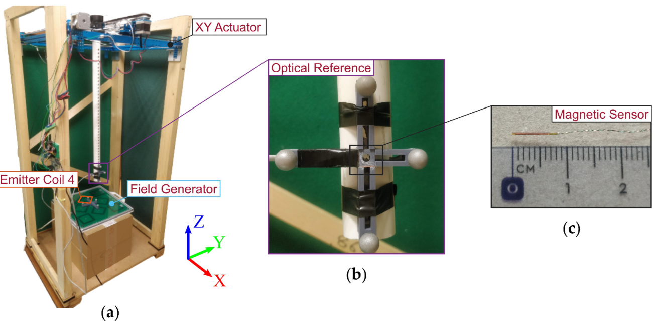
3.4. Experimental Tracking Test

A real electromagnetic tracking test was performed, where the four models introduced in Section 3.3 were used to resolve the position and orientation of a miniature clinical sensor (610158, Northern Digital Inc., Waterloo, ON, Canada). The elongated inductive coil is 0.45$\mathrm{mm}$ in diameter and 8.2 $\mathrm{mm}$ in length, as shown in Figure 3c.

Two sensor coils were used for the experiment, oriented with the Y and Z axes of the field generator, as they are defined in Figure 3a. Sensors were glued onto a 3D printed support [34], which was also used to host the passive spheres of the Polaris Vega optical system (Northern Digital Inc., Waterloo, Canada), for position and orientation reference. The frame with the magnetic sensors and the optical markers is shown in Figure 3b.

The two magnetic sensors were moved by an automated motorised system on a grid of $26\times 26$ points in a $25\times 25$${\mathrm{cm}}^2$ XY plane, placed approximately 15$\mathrm{cm}$ above the field generator, as shown in Figure 3a.

For every field measurement, the sensors were kept steadily at the test position and 40 values were collected. The noise level was estimated from both the standard deviation of the 40 measured signal values and from a frequency domain analysis, resulting in a signal-to-noise ratio (SNR) of 68$\mathrm{dB}$ in the first case and of 67$\mathrm{dB}$ using the second approach. In this experiment, the random error due to the jitter noise was removed by averaging the 40 measured values, to isolate the systematic error of the EMT system, caused by inaccurate field modelling of the field generator or introduced by the acquisition hardware [21].

The experimental magnetic measurements were used to find the sensor pose by minimising the difference, in a least-squares sense, between the eight flux measurements and the values predicted by the model at the estimated position and orientation. Electromagnetic tracking errors were calculated with respect to the optical tracking ground truth.

3.5. Long Flexible Inductive Sensor

As a possible application of the new formulation presented in this article, we proposed a long inductive coil, wound around a flexible surgical instrument, such as a guide-wire or a catheter. The benefits of such a sensor would be high sensitivity, due to the length and large cross-sectional area, linearity, due to the absence of a ferrite core, and ease of manufacture [13].

The difficulties in localising a long inductive sensor in real-time arise from the fact that the sensed field predictions must be calculated from the line-integral of the magnetic flux density along the coil axis, as per Equation (3), which has to be evaluated numerically and might be inaccurate as well as slowing computation. It is worthwhile to mention that it is possible to calculate the integral of Equation (3) without knowing the shape of the coil axis because, in the region considered, the magnetic field is curl-free and therefore any integration path connecting the two end-points is equivalent. The straight line defined by the two end-points could be used for simplicity.

Alternatively, the scalar potential formulation expressed in Equation (8) directly gives the exact analytical integral, which is then compared to the measured magnetic flux to find the position of the coil end-points. The sensor shape remains unknown because it cannot be deduced from the electromagnetic measurement, but if the sensor is moving in a line, as can be assumed for most endoscopic applications, it can be inferred from the passage constraints, i.e. from imaging, or from consecutively tracked end-point positions.

In this preliminary experiment, a flexible sensor shape was arbitrarily defined as:

$$\left[\begin{array}{c}x\hfill \\ y\hfill \\ z\hfill \end{array}\right]=\left[\begin{array}{c}25cos\left(3\pi /2t\right)\\ 25sin\left(3\pi /2t\right)\\ 100+50t\end{array}\right]\mathrm{mm};\mathrm{with}0\le t\le 1.$$

(22)

The sensor axis consisted of a loop of radius 25$\mathrm{mm}$, ranging from 100 to 150$\mathrm{mm}$ above the field generator, as drawn in Figure 4.

The total length of the sensor can be calculated as follows:

$$L={\int }_0^1\sqrt{{\left(-25\frac{3\pi }{2}sin\theta \right)}^2+{\left(25\frac{3\pi }{2}cos\theta \right)}^2+{50}^2}dt=\sqrt{{\left(25\frac{3\pi }{2}\right)}^2+{50}^2}\approx 128\mathrm{mm}.$$

(23)

Eight simulated flux measurements were calculated using the full-length magnetic model presented in this article. The values obtained were confirmed by the single-point model, integrated along the sensor axis using the MATLAB integral function, which makes use of adaptive quadrature methods.

The robustness of the proposed tracking algorithm was evaluated by adding Gaussian noise to the simulated flux measurements, and studying how the noise affected the position solutions. The noise level was selected to be 63$\mathrm{dB}$ below the magnitude of the simulated signal, in accordance with the signal-to-noise ratio measured in the real experiment of Section 3.4.

4. Results

This section presents the results of the experimental method described in Section 3. The study on the interpolation performance allowed us to choose a table of the magnetic scalar potential and a table of the three field components that are approximately equivalent in terms of position accuracy and table size. Then, the results of the simulated and real electromagnetic tracking tests are reported. In the end, the stability of the proposed tracking algorithm for long, flexible coils is shown using position error confidence regions.

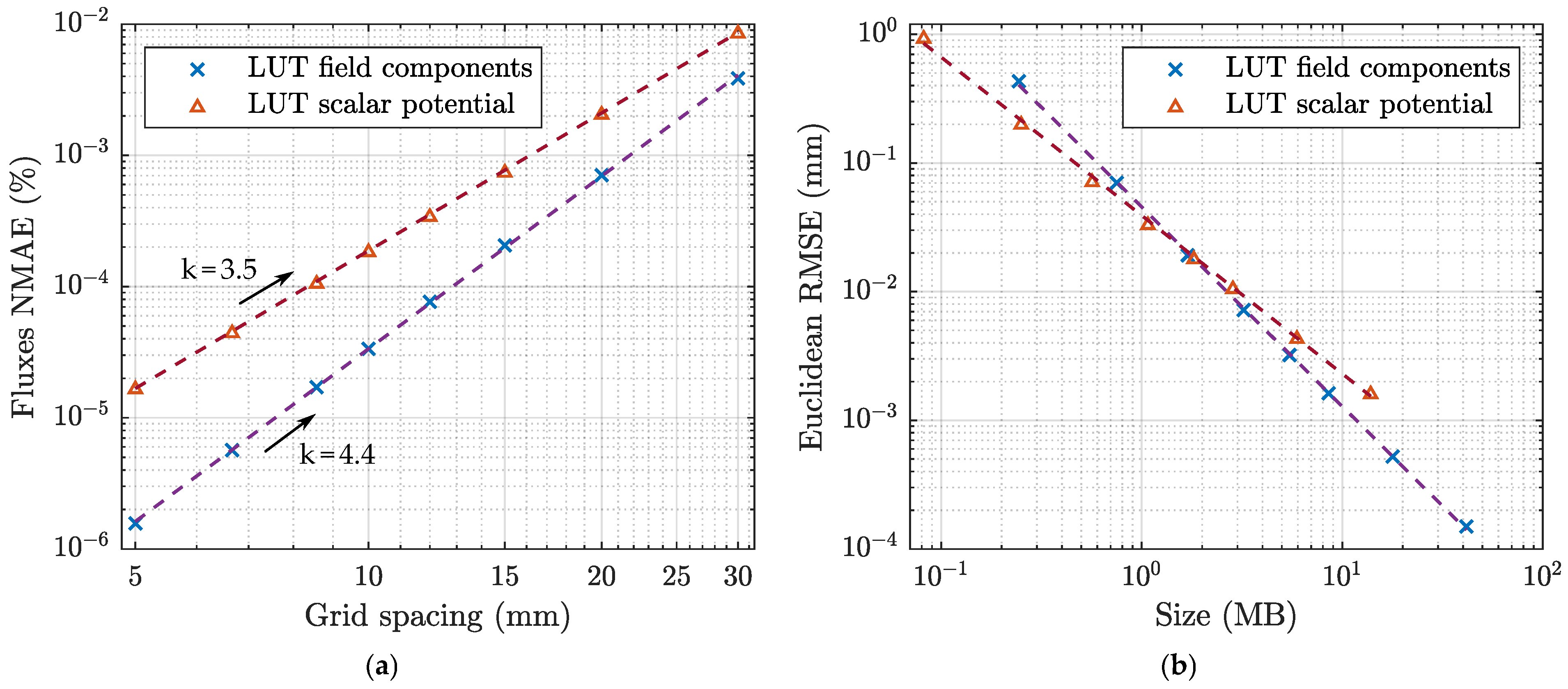
4.1. Model Interpolation

The interpolation and position errors of the two tabulated models introduced in Section 3.2 are plotted in Figure 5 for the different grid sizes analysed.

The interpolation error was expected to be proportional to the distance between the data points to the power $n+1$, where n is the degree of the interpolation polynomial [35]. As shown in Figure 5a, the power-law dependence is confirmed, where the best-fit exponents resulted in 3.5 and 4.4, for the two interpolated models respectively.

The magnetic fluxes obtained from the magnetic scalar potential are interpolated by a quadratic spline because they are calculated from the gradient operation, which involves first derivatives and makes the order of the polynomial one degree lower. Conversely, the cubic spline is maintained for the magnetic fluxes obtained from the magnetic field component-wise interpolation.

The average position error is shown in Figure 5b for the two tabulated models as a function of the table size. The two curves intersect approximately at 20$\mathsf{\mu }\mathrm{m}$, where the storage requirement is around 2$\mathrm{MB}$, which corresponds to a grid spacing of 1$\mathrm{cm}$ ($31\times 31\times 31$ grid-points) for the scalar potential table and of 1.5$\mathrm{cm}$ ($21\times 21\times 21$ grid-points) for the field components table. The two associated LUTs were selected for the models LUT FL (full-length) and LUT SP (single-point) used in the simulated and experimental tracking tests presented in this article.

4.2. Simulated Tracking Test

The results of the simulated tracking test described in Section 3.3 are reported in

Table 1. Model comparison, based on a simulation of a 10$\mathrm{mm}$-long sensor placed at 100,000 random positions and orientations within the tracking region. The normalised mean absolute error (NMAE) of the magnetic field, $\mathbf{H}$, is averaged between the eight equal emitter coils, and the associated error in terms of position accuracy, P, is reported. The error introduced by the single-point approximation is calculated with respect to the full-length model. Each LUT is evaluated against the correspondent analytical model.

Model	Full Length	Single Point	LUT FL	LUT SP
Time ($\mathsf{\mu }$ s)	44.3	74.8	22.8	33.7
$\mathbf{H}$, NMAE (‰)	—	0.0169	0.0015	0.0019
P, RMSE (mm)	—	0.098	0.018	0.018
P, PRC95 (mm)	—	0.161	0.025	0.031
Size (MB)	—	—	1.8193	1.6965

, comparing the full-length and single-point models, and the associated interpolated models LUT FL and LUT SP.

As explained in Section 4.1, the two LUTs were chosen to be approximately equivalent in terms of position RMSE and table size, and the results, in fact, demonstrate similar performance, with a 95% percentile (PRC95) of the position error of approximately 0.03$\mathrm{mm}$ in either case.

The effect of the single-point approximation is evaluated with respect to the full-length model. The position error PRC95 of the 100,000 test locations is below 0.2$\mathrm{mm}$, demonstrating a minimal difference between the two models.

The two analytical models were computationally more expensive than the correspondent tabulated models, with an average evaluation time that was approximately halved in either case when using a LUT. The analytical full-length model, based on the calculation of the magnetic scalar potential, was 1.7 times faster than the single-point model, based on the calculation of the three components of the magnetic field vector.

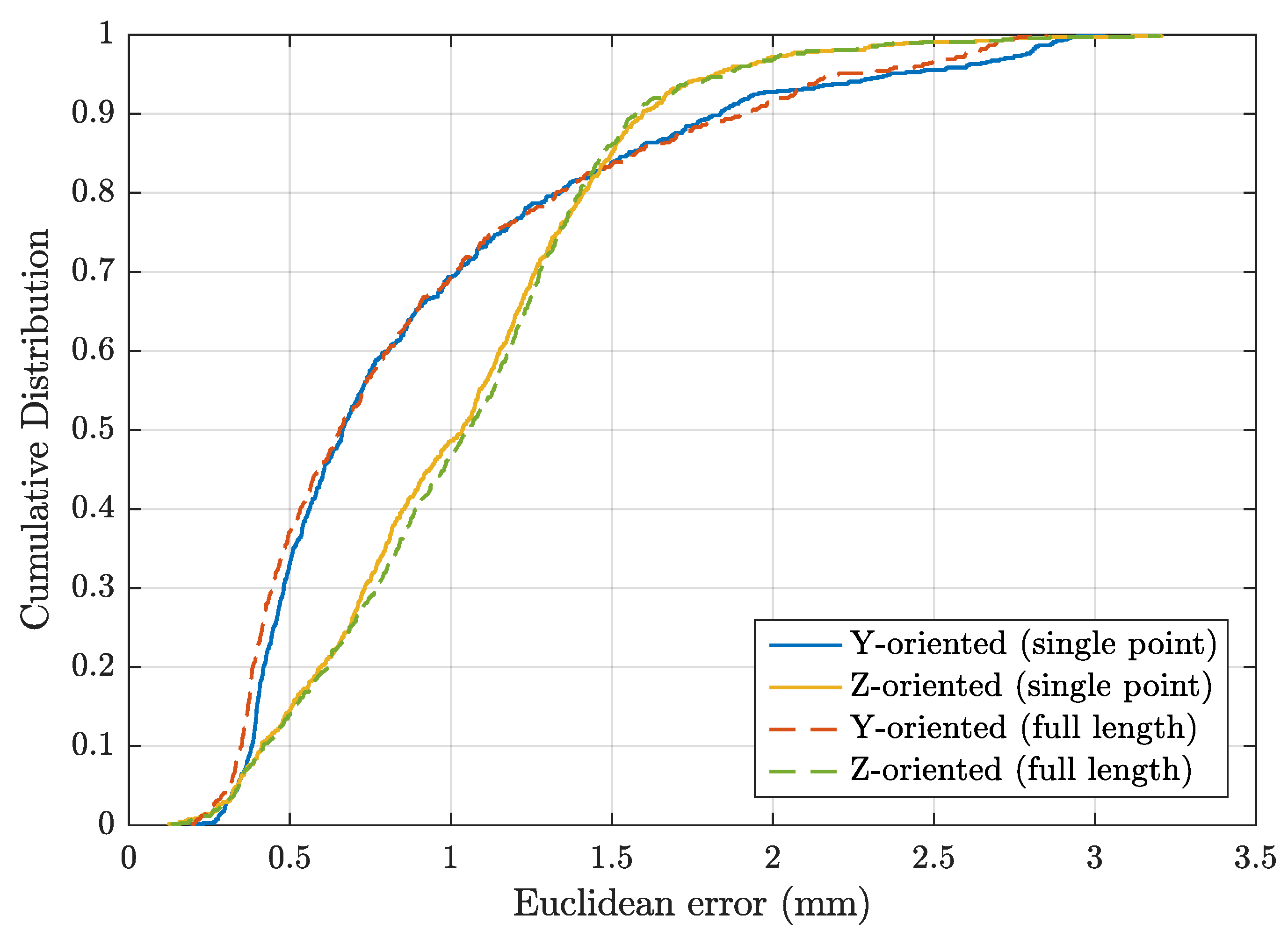
4.3. Experimental Tracking Test

As demonstrated by the results of Section 4.2 above, for sensors of the length of 10$\mathrm{mm}$ and the spatial variation of the magnetic field in the region considered, the full-length and the single-point models are almost equivalent in terms of accuracy, although the full-length model is on average faster.

The position error is compared for the two analytical models and the two sensor orientations in Figure 6, where the empirical cumulative distribution function (CDF) of the Euclidean error is plotted. The two tabulated models are not shown because they give almost exactly the same results as the associated analytical model, as can be verified from the error statistics reported in

Table 2. Average positional and angular errors of a real electromagnetic tracking experiment, where the full-length and the single-point analytical and tabulated magnetic models are compared. Errors are calculated with respect to optical tracking ground-truth.

Model	Full Length	Single Point	LUT FL	LUT SP
Y-oriented
RMSE (mm/deg)	1.08/0.70	1.10/0.70	1.08/0.70	1.10/0.70
ME (mm/deg)	0.88/0.49	0.90/0.49	0.88/0.49	0.90/0.49
PRC50 (mm/deg)	0.65/0.30	0.66/0.30	0.65/0.30	0.67/0.30
PRC95 (mm/deg)	2.20/1.64	2.36/1.69	2.20/1.64	2.35/1.69
Z-oriented
RMSE (mm/deg)	1.15/0.87	1.14/0.87	1.15/0.87	1.14/0.87
ME (mm/deg)	1.05/0.78	1.03/0.77	1.05/0.78	1.03/0.77
PRC50 (mm/deg)	1.05/0.80	1.04/0.80	1.05/0.80	1.03/0.80
PRC95 (mm/deg)	1.86/1.44	1.82/1.45	1.86/1.45	1.82/1.45

.

Although a small difference can be observed in Figure 6 when using the two alternative magnetic model formulations, this is completely irrelevant if compared to the main CDF error curve. In EMT surgical applications, other sources of error are dominant, such as thermal noise, metallic distortions, patient movements, and systematic errors in the system.

4.4. Long Flexible Inductive Sensor

The noise resilience of the proposed tracking method of a long coil is evaluated by propagating the errors from the simulated flux to the sensor end-points’ positions.

The Gaussian noise was assumed to be uncorrelated for the eight field frequencies, resulting in a diagonal $8\times 8$ covariance matrix, ${\Sigma }_{\mathrm{\Phi }}$. The positions of the end-points include six degrees-of-freedom (6DoF), which constitute the vector $\mathbf{p}\in {\mathbb{R}}^{6\times 1}$:

$$\mathbf{p}=\left[x_A,y_A,z_A,x_B,y_B,z_B\right]$$

(24)

where x, y and z, subscript A and B, are the Cartesian coordinates of the two end-points respectively, as defined in Figure 4.

The position covariance matrix, ${\mathrm{\Sigma }}_{\mathbf{p}}$, was obtained by the propagation of uncertainty theory, as given by Equation (25):

$${\mathrm{\Sigma }}_{\mathbf{p}}={\mathbf{J}}_{\mathbf{p}}^{+}·{\mathrm{\Sigma }}_{\mathrm{\Phi }}·{\mathbf{J}}_{\mathbf{p}}^{+}T$$

(25)

where ${\mathbf{J}}_{\mathbf{p}}^{+}$ is the Moore–Penrose inverse of the Jacobian matrix introduced in Section 3.1, for the flux values calculated in p.

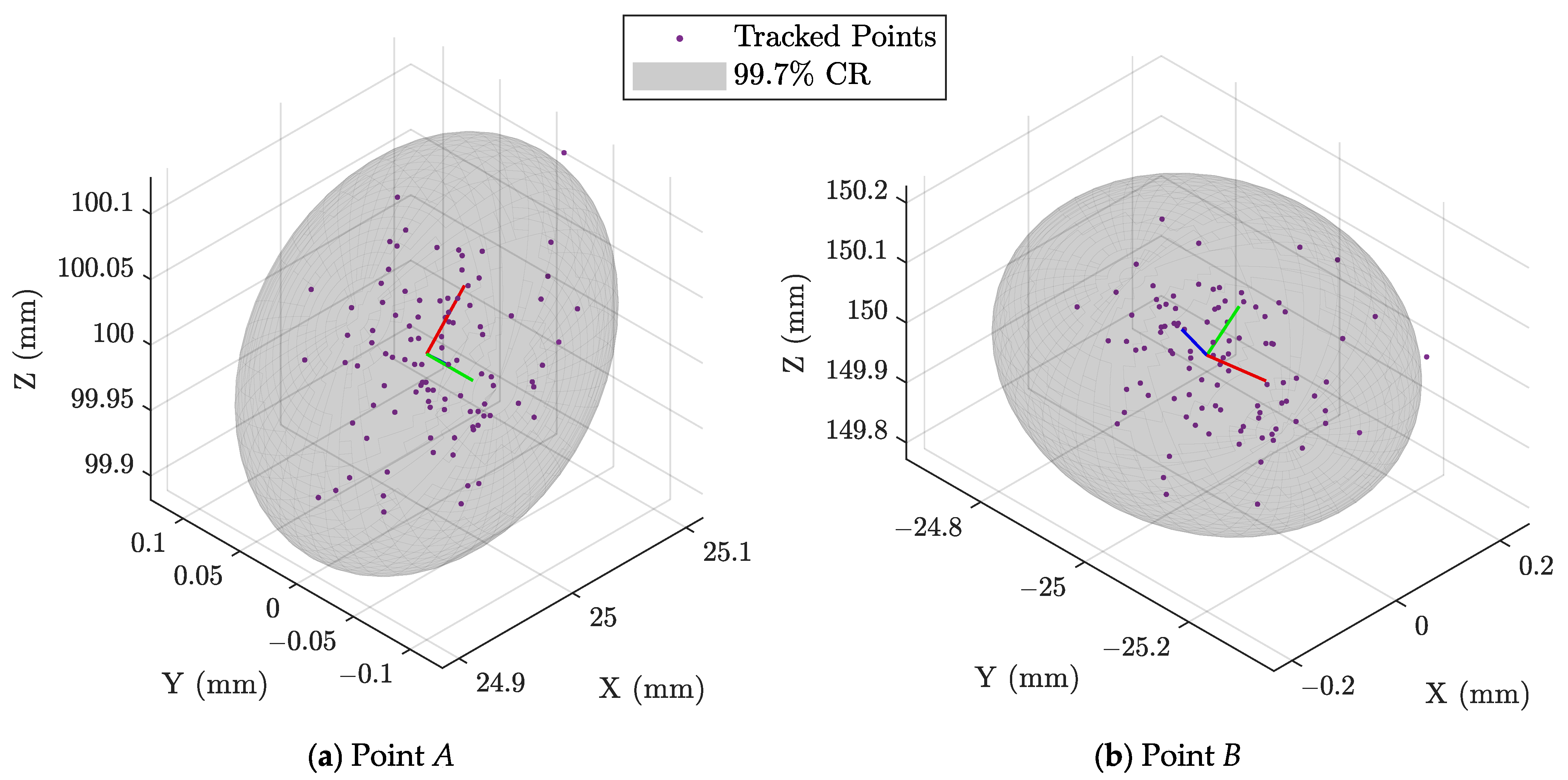
A number of 100 solution vectors p were sampled from the multivariate Gaussian distribution with covariance matrix ${\mathrm{\Sigma }}_{\mathbf{p}}$, and they are visualised separately in Figure 7, for the end-points A and B.

The total variation in the end-points perturbed positions can be quantified by two independent trivariate Gaussian distributions, which can be visualised through the associated ellipsoidal confidence regions to make immediately clear the worst position error directions. The values of 0.049$\mathrm{mm}$ and 0.12$\mathrm{mm}$ were obtained for the position standard deviation in the worst direction, for the solutions of points A and B respectively.

5. Discussion

In this section, the main results and findings obtained in this work are commented upon and their implications and future research directions are highlighted.

5.1. Model Interpolation

A method was presented to evaluate the model interpolation error in terms of electromagnetic tracking accuracy and it was applied to the Anser EMT field generator in order to compare the existing model based on the magnetic field vector with the new scalar potential formulation presented in this article.

The analysis demonstrated that the two models are equivalent in terms of storage requirements when the position error due to the interpolation approximation is approximately 20$\mathsf{\mu }\mathrm{m}$. If more accuracy is required, the table of the three field components takes less space, when the same interpolation performance is maintained. However, electromagnetic tracking accuracy is in general between 0.1$\mathrm{mm}$ and 1$\mathrm{mm}$, in which case the table of the magnetic scalar potential has a smaller size.

The choice of the model formulation and interpolation grid size must be evaluated specifically for the field generator to be modelled, the maximum interpolation error desired, the storage and memory availability, and the time requirements. The methodology presented in this article can be followed to find the optimal solution for the specific application.

It should be noted that further optimisations would be possible to reduce the look-up table size while maintaining the same interpolation performance, for example by using different grid-points for each emitter coil, possibly with cylindrical coordinates around the coil axis and adaptive spacing in the Z direction, or by considering different sub-regions where the grid spacing is selected based on the local magnetic field spatial variation. This could be useful for implementation of the tracking algorithm in embedded systems, but it is beyond the scope of this article, where it is assumed that the software runs on a computer machine, for which the tables analysed can be fully loaded into RAM.

5.2. Simulated and Experimental Tracking Tests

The simulated and the experimental tracking tests demonstrated similar results for the magnetic field model formulations compared.

The tabulated models proved to be approximately two times faster than the corresponding analytical model, although both the analytical and the tabulated models met the speed requirements for real-time electromagnetic tracking.

The experiments demonstrated that, for an inductive sensor of 10$\mathrm{mm}$ in length, the single-point approximation is in practice equivalent to the full-length model within the tracking volume considered. In other words, this means that the spatial variation of the magnetic field of the Anser EMT field generator is almost linear within the sensor length, at the test-points considered.

The single-point approximation introduces errors that increase with the sensor length, the field gradient rate of change, and the proximity to the field generator. In such cases, the novel full-length model introduced in this work must be used.

5.3. Long Flexible Inductive Sensor

A method for the electromagnetic tracking of a 128$\mathrm{mm}$-long inductive sensor was presented. The method can find the position of the sensor end-points, while the sensor shape remains unknown. The shape may usually be inferred from the passage constraints or precedent end-points positions. More advanced shape reconstruction techniques include the use of mathematical models [36,37], fluoroscopic images, or shape sensing based on the Fiber Bragg Grating [38]. Future work will include sensor manufacturing, electromagnetic tracking validation, and the development of a shape detection algorithm.

A robustness test was carried out, where a realistic noise level was added to simulated magnetic measurements, and the effect on the tracking results was shown. The test was used to predict the expected jitter noise of the electromagnetic tracking positions of the flexible sensor, due to random errors in the magnetic flux measurements, and shows the noise resilience of the proposed tracking method and algorithm. Systematic errors, such as the accuracy of the long-sensor model presented, must be evaluated by means of a real test and they will be assessed in future work.

6. Conclusions

In this article, a magnetic scalar potential formulation was studied for application in EMT systems. The formulation resolves the non-zero length ambiguity of elongated tracking sensors and demonstrated improvements in terms of speed and storage requirements.

Based on the magnetic scalar potential formulation, a novel model was introduced for the Anser EMT field generator and experiments were carried out to compare the new and the existing models.

The new model remains accurate even when the assumption of a single-point sensor is not true, for example for long sensors near the field generator or if high-gradient field generators are used to improve the tracking resolution.

The method might enable the use of longer tracking sensor coils, which can achieve higher sensitivities possibly without the requirement of a magnetic core, with advantages in terms of linearity, larger dynamic range, lower production costs, and increased flexibility.