Abstract
The nonuniform magnetic vortex gyrotropic oscillations along the cylindrical dot thickness were calculated. A generalized Thiele equation was used for describing the vortex core motion including magnetostatic and exchange forces. The magnetostatic interaction was accounted for in a local form. This allowed reducing the Thiele equation of motion to the Schrödinger differential equation and analytically determining the spin eigenmode spatial profiles and eigenfrequencies using the Liouville–Green method for the high-frequency modes. The mapping of the Schrödinger equation to the Mathieu equation was used for the low-frequency gyrotropic mode. The lowest-frequency gyrotropic mode transformed to the dot faces localized mode, increasing the dot thickness. The vortex gyrotropic modes are described for a wide range of the dot thicknesses according to the concept of the turning points in the magnetostatic potential. This approach allows treating the vortex localized modes (turning points) and nonlocalized modes within a unified picture.
1. Introduction
There is a longstanding interest in the topological spin textures in small ferromagnetic particles and thin films, such as magnetic vortices [1,2], skyrmions [3,4,5], and hopfions [6,7]. The magnetic vortex is one of the simplest topologically nontrivial and stable spin textures in condensed matter physics. Since the vortex state of magnetization was discovered as the ground state of patterned soft magnetic dots [1], the dynamics of magnetic vortices attract considerable attention.
The vortex gyrotropic frequency and trajectory in circular magnetic dots were predicted by Guslienko et al. [8]. Being displaced from its equilibrium position in the dot center, the vortex core reveals sub-GHz frequency oscillations with a narrow linewidth. Then, existence of the vortex low-frequency gyrotropic mode dominated by the dipolar interaction was observed experimentally by different experimental techniques [9,10,11]. The experimental study of magnetic vortex dynamics was started in 2003 using time-resolved Kerr microscopy [9] and X-ray imaging [10]. Then, Novosad et al. [11] demonstrated that, upon being shifted from its equilibrium position by a microwave field, the vortex core experiences oscillations with the eigenfrequency proportional to the dot thickness/radius aspect ratio β = L/R. Later, it was shown that similar microwave-frequency oscillations with extremely narrow linewidth could be excited by DC spin polarized current [12,13]. Lastly, a large microwave generation from the current-driven magnetic vortex oscillators was observed in magnetic tunnel junctions [14]. These results allow considering the magnetic vortex gyrotropic motion as an important excitation mode of the spin torque nano-oscillators (STNO) in layered nanopillars and nanocontacts [15].
The magnetic vortex excitations in patterned films have been studied extensively for the last decades. However, in all experiments conducted in 2003–2013 the observed vortex gyrotropic modes had a uniform profile along the dot thickness accounting for the dot thickness being relatively small (typically, 20–30 nm). The nonuniform along-thickness vortex core mode was first simulated micromagnetically by Boust and Vukadinovic for small-radius circular dots [16]. The mode frequency decreases with dot thickness L increasing approximately as . A model of the vortex core position inhomogeneous along the dot thickness was developed [17], which principally explained this behavior as a consequence of the exchange interaction in the out-of-plane z-direction. Then, the existence of higher-order vortex gyrotropic modes was demonstrated by micromagnetic simulations for thick (60–80 nm) submicron rectangular prisms [18]. These modes were described schematically as oscillations of the vortex core line with several nodes along the dot thickness (or oscillation modes of the asymmetric Bloch wall). Then, it was proven experimentally and confirmed by simulations and calculations that, in thick circular dots, these kinds of the vortex dynamical deformations, i.e., flexure oscillations of the vortex core string with n nodes along the dot thickness, can exist [19,20].
In this paper, a route from 2D to 3D magnetic soliton dynamics is considered conducting generalization of the 2D magnetic vortex strings to 3D topological spin textures. A third spatial dimension is added to 2D magnetic vortices, exploring the vortex gyrotropic modes in thick cylindrical dots and nanowires and considering the 3D vortex strings (tubes) oscillations. Specifically, the thickness-dependent magnetic vortex gyrotropic dynamics is calculated in the thick circular dots. A new analytic approach to the problem is developed, allowing the vortex eigenfrequencies and gyrotropic mode profiles to be calculated. The proposed analytical theory is based on the Thiele equation of motion of the soliton center and turning points of the vortex core motion along the dot thickness. The theory describes the whole vortex gyrotropic spectra in a circular dot, accounting for the exchange and magnetostatic energies.
2. Theory
2.1. Stability of the Magnetic Vortex State in Cylindrical Geometry
Let us consider a cylindrical dot (wire) of radius R and thickness (wire length) L made of soft magnetic material like Permalloy (NiFe alloy). Let us also assume that the dot (wire) radius , where is the material exchange length, to allow the vortex state energy minimum (A is the exchange stiffness, and is the saturation magnetization). Then, following Usov et al. [21], the total dot magnetic energy, consisting of the exchange energy and magnetostatic energy of the face charges, can be minimized with respect to the vortex core radius, . The equilibrium vortex core radius at is approximately equal to , where 0.685. We are interested to find a border of the vortex state stability increasing the dot thickness, at , when the vortex state gradually transforms to a quasi-uniform out-of-plane magnetized state (quasi-uniform state magnetized along the nanowire length if , ). The simplest estimation of the critical thickness for such a transition is , i.e., . However, more careful analysis based on the vortex equilibrium magnetic energy and the vortex “half-skyrmion” ansatz [21] allows writing down a more exact value of the critical thickness (wire length) as . For the typical material parameters 14 nm and the nanodot (nanowire) radius 60 nm, the critical length is 2.36 μm. It is assumed here that the dot (wire) static magnetization is uniform along the thickness (length) coordinate. If any nonuniformity along the thickness is accounted for, then the critical value of can be smaller. An example of such nonuniformity is an “end-vortex” state, when the magnetization configuration is vortex-like near the nanowire ends (dot faces) and almost uniform (along the wire length) in the wire main part. Nevertheless, for the given dot radius , there is a wide interval of the dot thickness (wire length) where the vortex state is stable. The minimal value of for the given dot radius R is several hundred nanometers. The typical dot radius is 100–300 nm. Therefore, we can safely consider that the dots with the aspect ratio are in the single vortex state and consider excitations over this ground (metastable) magnetization background. Such large values of the dot thickness nm correspond to the extension of the vortex stability region above the value of calculated in [22].
2.2. The Generalized Thiele Equation of Motion of the Magnetic Soliton Center
Circular dots (wires) made of soft magnetic material have a vortex state of magnetization as the ground state for a certain dot radius R and thickness L. To calculate the vortex state excitation frequencies, the Landau–Lifshitz–Gilbert (LLG) equation of motion is used, which describes the evolution of magnetization in a ferromagnet in the presence of an effective magnetic field and damping. It is written in the following form:
where γ is the gyromagnetic ratio, is the dimensionless damping constant, and is the saturation magnetization. The effective field is a combination of the external magnetic field, exchange field, the demagnetizing field, etc., where is the total magnetic energy density. It was shown by Thiele [23] that, for a description of the dynamics of magnetic domains (solitons), the LLG equation can be rewritten in another form that allows simplifying the calculations. Thiele’s approach is applicable to describe the dynamics of stable magnetization configurations (magnetic solitons) that can be characterized by a position of their center (a collective coordinate) that can vary with time. Let us use a cylindrical coordinate system with the cylinder axis directed along the z-axis. To consider the thickness-dependent vortex excitations, it is assumed that the magnetization as a function of the coordinates , and time can be written in the form The two-dimensional vector represents oscillations of the vortex core string in the dot xy-plane for a given value of z. Then, neglecting the damping, we can rewrite the LLG equation as the Thiele equation,
where is the total magnetic energy of the dot, and . Introducing the unit vector of magnetization , the components of the gyrotensor density per unit dot thickness related to 2D topological charge of the spin texture can be defined as follows:
We can apply Thiele’s approach for the magnetic vortex motion in a circular dot (cylindrical wire). The vortex core position is defined in dimensionless units as (). The magnetization has the following components: and , where is a complex function of the complex coordinate and its complex conjugate , and is the vortex core polarization [2]. Inside the vortex core the vortex configuration is described as a 2D topological soliton, i.e., , where an analytic function satisfies the condition . The vortex core position s in the xy-plane corresponds to a zero of the function . Outside the vortex core region, where , the magnetization distribution is described by the function . The function corresponds to the description of magnetic vortex as a nonlocalized topological soliton. The magnetostatic energy plays an essential role for the magnetic vortices in restricted geometries. Therefore, for describing the vortex dynamics, a two-vortex model (no side surface charges induced in the course of motion) is used with the analytical function being written as [2,8], where is the vortex chirality, and is the reduced vortex core radius. It is assumed that the dependence of magnetization on the thickness coordinate z is accounted for via the function . The vortex core with the radius should be accounted for explicitly in the case of dots (nanowires) with radii R of several tens of nanometers.
The righthand-side term in Equation (2) is the variational derivative of the total magnetic energy of the dot with a displaced magnetic vortex centered in a point taken with respect to the vortex core coordinate . The total magnetic energy W consists of the magnetostatic, exchange, and Zeeman energies and can be calculated as a function of s. The magnetostatic energy consists of the energy of volume magnetic charges , energy of the side surface charges, and energy of the dot face (wire end) charges. The side surface charges are absent for the selected vortex model. The face charges related to the magnetization component contribute only to the boundary conditions at the dot faces . Therefore, the magnetostatic energy is related with the volume magnetic charges and can be written in the following form:
The exchange energy is with A being the exchange stiffness parameter. Integration over the in-plane dot coordinates and neglecting the vortex core contribution () yields, in the quadratic approximation on the small parameter , the nonlocal magnetostatic energy,
where the magnetostatic kernel is , , , and is the dot volume. The thickness coordinate z is in units of L.
The exchange energy is
where is the in-plane and is the out-of-plane exchange stiffness coefficient calculated within the model, and is the reduced vortex core radius.
The generalized Thiele equation of motion (Equation (2)) is
where is the gyrovector per unit dot thickness, , , and .
Assuming circular motion of the vortex core with the frequency (or making a Fourier transform with respect to time t for the variable ), the Thiele equation can be written as a two-component differential–integral equation containing nonlocal terms,
for the vector components, where , and .
Equation (8a) should be amended by the boundary conditions at the dot faces . This equation can be written in the compact form , where the linear integral–differential operator is defined by the righthand side of Equation (8a). Equation (8a) allows finding eigenmodes of the vortex core string oscillations and corresponding eigenfrequencies , which are expressed via the eigenvalues . It is convenient to write Equation (8a) in the dimensionless form, dividing both parts of the equation by . Then, the eigenvalue λ corresponds to the dimensionless frequency , where . The value of is 30 GHz for a typical composition of alloy with 0.80 ( 800–860 kA/m).
It is convenient to introduce a complex circular variable . The equation of motion for has the form
The solution of Equation (8b) yields the complex eigenfunctions and eigenfrequencies of the vortex string oscillations. The absolute value and the phase of the n-th eigenmode as are introduced. It is determined from the symmetry of Equation (8b) that the eigenfunctions satisfy the condition , which is equivalent to the conditions and . Then, the time dependence of the vortex displacement vector components is given by the equations , . Equation (8b) has pure real (even) solutions or pure imaginary (odd) solutions , if the phases or , respectively.
The aim is to find analytical solutions of Equation (8a), the eigenfrequencies and eigenfunctions of the operator numbered by the integer index n = 0, 1, 2, … The problem is that there is no theory of the linear integral–differential equations. Therefore, we reduce Equation (8a) to a local form, i.e., a differential equation for the function . The kernel has a sharp maximum at if the dot aspect ratio is large enough. This allows substituting in the magnetostatic term containing the kernel to and writing the Thiele equation in the form of the differential Schrödinger equation with an effective potential energy,
where .
The function can be calculated explicitly and has the form . has a smooth maximum at , in the dot middle plane, and minima at the dot faces, . The potential at a small dot aspect ratio . However, upon increasing , the function reveals more and more pronounced minima at . Such minima result in the low-frequency (n = 0) eigenmode localization near the dot faces increasing the dot thickness or the dot aspect ratio at the fixed dot radius R. The accuracy of the local approximation, Equation (9), increases with increasing.
We can rewrite Equation (9) in the standard oscillator-like form for both vortex core displacement s components,
where a small thickness-independent coefficient μ is included in the eigenvalue λ.
3. Magnetic Vortex String Gyrotropic Dynamics
3.1. The Lowest Frequency Gyrotropic Mode
Starting from Equation (10), it is possible to satisfy, for a given λ, the condition , which corresponds to the classical turning points located somewhere near the dot faces. Other turning points appear naturally due to the restricted dot geometry. More detailed analysis shows that the turning points exist only for the lowest eigenvalue . In other words, the lowest frequency eigenmode is localized between the turning points and ½ (or and −½) near the dot top/bottom surfaces. The mode frequency is within the interval shown in Figure 1. This interval is very narrow for small and rapidly increases with increasing. Another estimation of the lowest mode gyrofrequency valid at small << 1 can be obtained assuming the mode uniformity along the dot thickness, i.e., putting s in Equation (10). This frequency was calculated in [8] as .
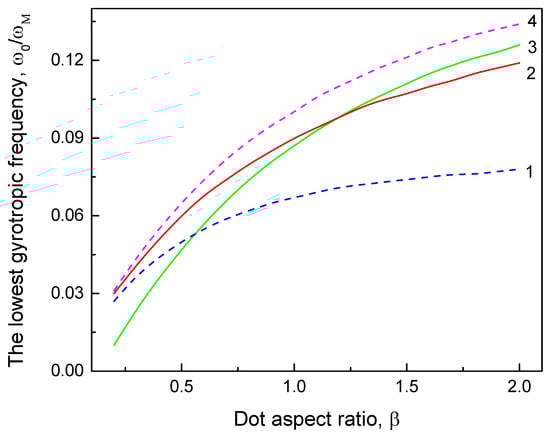
Figure 1.
The lowest vortex gyrofrequency (solid line 3) calculated using Equation (12a). The dashed lines 1 and 4 describe the limiting frequencies corresponding to the frequency window of the mode localization between the turning points. The frequency (solid line 2) is the gyrotropic frequency calculated in [8] assuming the gyromode uniformity along the dot thickness extrapolated for large values of β. The reduced dot radius .
We approximate the magnetostatic potential in Equation (10) as . This allows rewriting Equation (10) in the form of the Mathieu equation [24,25],
where , , and . The fitting parameter p is defined as and is a function only of β.
The solutions of the Mathieu equation are known. We are interested to use only the lowest eigenvalue of Equation (11), which is the increasing function of the parameter q. q is an increasing function on β (the dot radius R is fixed). For the values of q > 1, the eigenvalue of the Mathieu equation is defined approximately by the function [24,25], where , is the reduced dot radius, and . For instance, if the value of is used, then at , and . The eigenvalue corresponds to the lowest gyrotropic mode eigenfrequency (see Figure 1),
and the corresponding eigenfunction is the zero-order Mathieu even function . For the large values of the parameter q >> 1, such an eigenfunction (not normalized) can be represented in the following form [24,25]:
The even function for the typical dot sizes is shown in Figure 2, where the normalized eigenfunctions , are plotted for different values of β. The degree of the lowest gyrotropic mode localization at the dot faces increases with increasing dot thickness. The lowest mode eigenfrequency given by Equation (12a) is asymptotically correct at the large values of the parameter q, i.e., for thick enough dots (q > 12.8 at > 0.5, r = 10). The frequency is lower than the gyrotropic frequency calculated within uniform along thickness mode approximation in [8] at intermediate values of and practically coincides with at large values of . The approximation of by the Mathieu method (Equation (12a)) is not applicable at small values of q (small ). It leads to underestimation of the lowest mode frequency in comparison with the homogeneous solution .
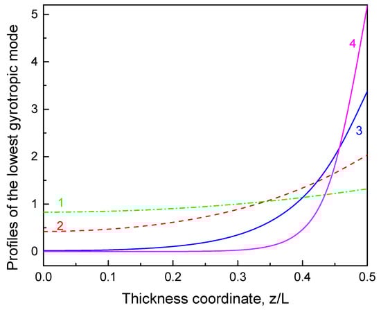
Figure 2.
The normalized profiles of the lowest vortex gyrotropic mode calculated using the Mathieu function approximation, Equation (12b). The values of the dot aspect ratio β: 0.3 (1), 0.5 (2), 1.0 (3), and 2.0 (4). The reduced dot radius .
3.2. High-Frequency Vortex Gyrotropic Modes
Let us consider the equation of motion (Equation (10)) for higher frequencies, when there are no turning points for the function . If, additionally, we assume that the function is smooth enough, then the solution of Equation (10) can be written in the Liouville–Green approximation [26] as
where , are some constants, which can be defined by the boundary conditions at the dot faces, .
The function has sense of the amplitude, and has sense of the phase of the vortex string displacement used in the complex form . It is assumed that there is no surface magnetic anisotropy and no dipolar pining at the dot faces. Therefore, the natural exchange boundary conditions, at , are used. Equation (13) combined with these boundary conditions allows finding the vortex oscillation eigenfrequencies and explicit form of the eigenfunctions. It can be shown that solving the linear system of the equations for the coefficients , and the eigenfrequencies can be found from the equation
and the corresponding eigenfunctions are
where , , and are taken at .
The function rapidly decreases with the frequency increasing. It is different from zero solely due to the magnetostatic potential nonuniformity along the dot thickness. For thin dots (small values of ), and , , for all eigenmode numbers For the large values of , the condition is satisfied with a high degree of accuracy for all eigenmodes except the n = 1 mode. The phase difference for n = 1 mode decreases from 0.998 to 0.849 increasing from 0.2 to 1.0. Apparently, the condition corresponds to the simple exchange eigenfunctions and corresponding exchange-dominated eigenfrequencies can be written in the form of Equation (4) of the paper by Ding et al. [19]. .
The eigenfunctions are even at or odd at with respect to the dot middle plane z = 0 according to the general approach. The non-normalized eigenfunctions can be written in the form for the even modes and for the odd modes taken at . The normalized eigenfrequencies are shown in Figure 3 and the normalized eigenfunctions are plotted in Figure 4 for typical dot parameters. The following normalization was used: , . The eigenfrequencies with n = 2, 3, … rapidly decrease with the dot thickness L increasing at small β as approximately and approach some constant values at large β. The thickness dependence of the n = 1 mode is different. It reveals a smooth minimum at intermediate values of β. Another important peculiarity of the n = 1 vortex gyrotropic mode is that the mode frequency becomes close to the magnetostatic integral , increasing the aspect ratio β up to approximately 1.0; therefore, the function becomes very small, and the Liouville–Green approximation is no longer applicable. This corresponds to the regime of the frequency crossing between the lowest n = 0 () and n = 1 () vortex gyromodes and will be considered elsewhere.
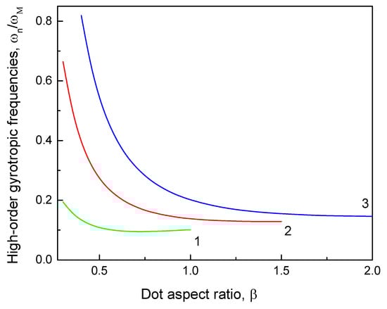
Figure 3.
The high-order vortex eigenfrequencies of the delocalized gyrotropic modes with the numbers n = 1, 2, and 3 calculated by Equation (14). The reduced dot radius .
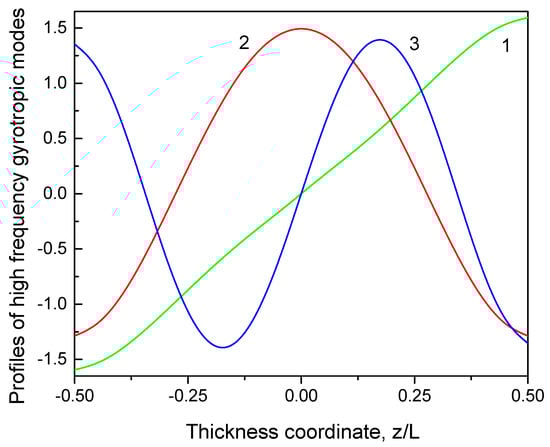
Figure 4.
The normalized eigenfunctions of the high-frequency vortex gyrotropic modes with the numbers n = 1, 2, and 3 calculated using the Liouville–Green approximation, Equation (15). The dot aspect ratio β = 1, and the reduced dot radius .
3.3. The Role of the Vortex Mass in the Gyrotropic Dynamics
The relationship of the eigenvalue parameter λ with the vortex gyrotropic frequency ω is more complicated if other high-order time derivatives of the vortex core displacement are accounted for in the Thiele equation of motion (Equation (7)). Formally, this can be achieved assuming a velocity-dependent soliton ansatz . It was shown in [27] that the mass term is, in general, nonlocal. If the vortex mass is accounted in a local approximation, then the equation of motion of the vortex center position is
where is the vortex mass per unit dot thickness, and is the dimensionless vortex mass.
In the case where Equation (16) is valid, the eigenvalue λ is represented by the function . If the spectrum of the operator Equation (8a) is found, then the eigenfrequency spectrum can be represented as . The reduced eigenfrequencies for any finite value of the vortex mass , i.e., accounting for the vortex mass, results in a reduction in all vortex gyrotropic frequencies . The vortex mass can be calculated via the vortex string coupling with the azimuthal spin wave modes having the azimuthal indices [27] according to the concept of the topological gauge field related to the vortex motion [28]. The interaction of the moving vortex core with the azimuthal spin waves was confirmed experimentally [29]. It was recently found that some extra azimuthal spin-wave modes having a curled structure at the dot top and bottom faces appear in the spin excitation spectrum when increasing the dot thickness [30]. Therefore, the calculation of the vortex dynamical mass in thick dots is a complicated problem. The frequency correction due to the vortex mass is small for thin dots [28]. However, the importance of the mass term drastically increases with the dot thickness L increasing in the range of 50–100 nm [27]. The Thiele equation of motion of the soliton center position X and the concept of the soliton mass were recently used to interpret the low-frequency skyrmion excitation modes in CoPt circular dots [31], where a giant value of the mass order of 10−21 kg was introduced.
4. Discussion and Conclusions
The magnetic vortex gyrotropic modes in thick cylindrical soft magnetic dots were described for a wide range of the dot thickness according to the concept of the turning points in the magnetostatic potential. This approach allows treating the vortex localized modes (turning points) and nonlocalized modes within a unified picture.
The lowest-frequency vortex gyrotropic mode () was calculated for the dot aspect ratios within the approach. The calculated frequency was lower than the gyrotropic frequency calculated within uniform along thickness mode approximation in [8] at intermediate values of (<1) and practically coincided with at large values of () (see Figure 1). The good accuracy of the expression for at large is a surprise because the lowest-frequency eigenmode depicted in Figure 1 is strongly inhomogeneous, localized at the dot faces at such values of . The frequency monotonically increases with increasing. This is in some contradiction with the measurements and simulations conducted in [19,27], where a smooth maximum of the dependence was obtained at . We can speculate that the maximum arises due to repulsing of the frequency branches of the lowest (n = 0) and the next (n = 1) vortex gyrotropic modes when the frequencies and are close to their crossing point [32]. The low-frequency eigenmode localization at the dot faces at large values of ( is due to strong nonuniformity of the magnetostatic potential near the dot top and bottom faces.
The calculated eigenfrequencies of the nonlocalized vortex string modes (n = 1, 2 …) follow the exchange-dominated decrease only for relatively small dot thicknesses and approach some constant values at large values of the dot aspect ratio β (see Figure 3). This effect is beyond the measurements/simulations conducted in [19,21] and should be verified. The eigenmodes are odd for n = 1, 3, … and even for n = 2, 4, … functions of the thickness coordinate z with respect to the dot middle plane (see Figure 4). The n = 1 mode profile deviates essentially from the simple function used in [19], and the deviation increases with the dot aspect ratio β increasing. The profiles of the high-order vortex gyrotropic modes , n = 2, 3, … are close to the standing plane waves supported by the dominating exchange interaction [19].
The vortex gyrotropic modes calculated here for thick circular cylinders are not specific to this dot shape. Similar magnetic vortex excitations should exist also for other dot shapes such as a dome shape or square/rectangular shape. The point is that the dot thickness should be large enough to allow 3D magnetization texture excitations. The inhomogeneous gyrotropic oscillations of the vortex core string can be considered as a step toward understanding the magnetic topological soliton dynamics increasing the system dimensionality from 2D to 3D.
Funding
The author acknowledges support by IKERBASQUE (the Basque Foundation for Science). The research was funded in part by the Spanish Ministry of Science and Innovation grant PID2019-108075RB-C33 /AEI/10.13039/501100011033 and by the Norwegian Financial Mechanism 2014–2021 trough project UMO-2020/37/K/ST3/02450.
Institutional Review Board Statement
Not applicable.
Informed Consent Statement
Not applicable.
Data Availability Statement
Not applicable.
Acknowledgments
The author thanks G.N. Kakazei and E.V. Tartakovskaya for discussions.
Conflicts of Interest
The author declares no conflict of interest.
References
- Shinjo, T.; Okuno, T.; Hassdorf, R.; Shigeto, K.; Ono, T. Magnetic vortex core observation in circular dots of permalloy. Science 2000, 289, 930–932. [Google Scholar] [CrossRef] [PubMed] [Green Version]
- Guslienko, K.Y. Magnetic vortex state stability, reversal and dynamics in restricted geometries. J. Nanosci. Nanotechn. 2008, 8, 2745–2761. [Google Scholar] [CrossRef]
- Sampaio, J.; Cros, V.; Rohart, S.; Thiaville, A.; Fert, A. Nucleation, stability and current-induced motion of isolated magnetic skyrmions in nanostructures. Nat. Nanotechn. 2013, 8, 839. [Google Scholar] [CrossRef] [PubMed]
- Fert, A.; Reyren, N.; Cros, V. Magnetic skyrmions: Advances in physics and potential applications. Nat. Rev. Mat. 2017, 2, 17031. [Google Scholar] [CrossRef]
- Guslienko, K.Y. Magnetic vortices and skyrmions. J. Magnetics 2019, 4, 549–567. [Google Scholar] [CrossRef]
- Kent, N.; Reynolds, N.; Raftrey, D.; Campbell, I.T.G.; Virasawmy, S.; Dhuey, S.; Chopdekar, R.V.; Hierro-Rodriguez, A.; Sorrentino, A.; Pereiro, E.; et al. Creation and observation of Hopfions in magnetic multilayer systems. Nat. Commun. 2021, 12, 1562. [Google Scholar] [CrossRef]
- Tejo, F.; Hernández, H.R.; Chubykalo-Fesenko, O.; Guslienko, K.Y. The Bloch point 3D topological charge induced by the magnetostatic interaction. Sci. Reports 2021, 11, 21714. [Google Scholar] [CrossRef]
- Guslienko, K.Y.; Ivanov, B.A.; Novosad, V.; Otani, Y.; Shima, H.; Fukamichi, K. Eigenfrequencies of vortex state excitations in magnetic submicron-size disks. J. Appl. Phys. 2002, 91, 8037–8039. [Google Scholar] [CrossRef]
- Park, J.P.; Eames, P.; Engebretson, D.M.; Berezovsky, J.; Crowell, P.A. Imaging of spin dynamics in closure domain and vortex structures. Phys. Rev. B 2003, 67, 020403. [Google Scholar] [CrossRef] [Green Version]
- Choe, S.-B.; Acremann, Y.; Scholl, A.; Bauer, A.; Doran, A.; Sthr, J.; Padmore, H.A. Vortex Core-Driven Magnetization Dynamics. Science 2004, 304, 420–422. [Google Scholar] [CrossRef] [Green Version]
- Novosad, V.; Fradin, F.Y.; Roy, P.E.; Buchanan, K.S.; Guslienko, K.Y.; Bader, S.D. Magnetic vortex resonance in patterned ferromagnetic dots. Phys. Rev. B 2005, 72, 024455. [Google Scholar] [CrossRef] [Green Version]
- Pribiag, V.S.; Krivorotov, I.N.; Fuchs, G.D.; Braganca, P.M.; Ozatay, O.; Sankey, J.C.; Buhrman, R.A. Magnetic vortex oscillator driven by d.c. spin-polarized current. Nat. Phys. 2007, 3, 498–503. [Google Scholar] [CrossRef]
- Mistral, Q.; Van Kampen, M.; Hrkac, G.; Kim, J.-V.; Devolder, T.; Crozat, P.; Chappert, C.; Lagae, L.; Schrefl, T. Current-driven vortex oscillations in metallic nanocontacts. Phys. Rev. Lett. 2008, 100, 257201. [Google Scholar] [CrossRef] [PubMed] [Green Version]
- Dussaux, A.; Georges, B.; Grollier, J.; Cros, V.; Khvalkovskiy, A.V.; Fukushima, A.; Fert, A. Large microwave generation from current-driven magnetic vortex oscillators in magnetic tunnel junctions. Nat. Commun. 2010, 1, 8. [Google Scholar] [CrossRef] [Green Version]
- Guslienko, K.Y.; Sukhostavtes, O.V.; Berkov, D.V. Nonlinear magnetic vortex dynamics in a circular nanodot excited by spin-polarized current. Nanoscale Res. Lett. 2014, 9, 386. [Google Scholar] [CrossRef] [Green Version]
- Boust, F.; Vukadinovic, N. Micromagnetic simulations of vortex-state excitations in soft magnetic nanostructures. Phys. Rev. B 2004, 70, 172408. [Google Scholar] [CrossRef]
- Guslienko, K.Y.; Hoffmann, A. Field evolution of tilted vortex cores in exchange-biased ferromagnetic dots. Phys. Rev. Lett. 2006, 97, 107203. [Google Scholar] [CrossRef]
- Yan, M.; Hertel, R.; Schneider, C.M. Calculations of three-dimensional magnetic normal modes in mesoscopic Permalloy prisms with vortex structure. Phys. Rev. B 2007, 76, 094407. [Google Scholar] [CrossRef] [Green Version]
- Ding, J.; Kakazei, G.N.; Liu, X.M.; Guslienko, K.Y.; Adeyeye, A.O. Higher order vortex gyrotropic modes in circular ferromagnetic nanodots. Sci. Rep. 2014, 4, 4796. [Google Scholar] [CrossRef]
- Ding, J.; Kakazei, G.N.; Liu, X.M.; Guslienko, K.Y.; Adeyeye, A.O. Intensity inversion of vortex gyrotropic modes in thick ferromagnetic nanodots. Appl. Phys. Lett. 2014, 104, 192405. [Google Scholar] [CrossRef]
- Usov, N.A.; Peschany, S.E. Vortex magnetization distribution in a thin ferromagnetic cylinder. Phys. Met. Metallogr. 1994, 78, 591. [Google Scholar]
- Metlov, K.L.; Guslienko, K.Y. Stability of magnetic vortex in soft magnetic nano-sized circular cylinder. J. Magn. Magn. Mat. 2002, 242–245, 1015. [Google Scholar] [CrossRef] [Green Version]
- Thiele, A.A. Steady-state motion of magnetic domains. Phys. Rev. Lett. 1973, 30, 230. [Google Scholar] [CrossRef]
- McLachlan, N.W. Theory and Application of Mathieu Functions, 1st ed.; Dover: New York, NY, USA, 1964. [Google Scholar]
- Bateman, H. Higher Transcendental Functions; McGraw-Hill: New York, NY, USA, 1955; Volume 3. [Google Scholar]
- Olver, F.W.J. Introduction to Asymptotics and Special Functions; Academic Press: New York, NY, USA; London, UK, 1974. [Google Scholar]
- Guslienko, K.Y.; Kakazei, G.N.; Ding, J.; Liu, X.M.; Adeyeye, A.O. Giant moving vortex mass in thick magnetic nanodots. Sci. Rep. 2015, 5, 13881. [Google Scholar] [CrossRef] [PubMed] [Green Version]
- Guslienko, K.Y.; Aranda, G.R.; Gonzalez, J. Topological gauge field in nanomagnets: Spin-wave excitations over a slowly moving magnetization background. Phys. Rev. B Condens. Matter 2010, 81, 014414. [Google Scholar] [CrossRef] [Green Version]
- Park, J.P.; Crowell, P.A. Interactions of spin waves with a magnetic vortex. Phys. Rev. Lett. 2005, 95, 167201. [Google Scholar] [CrossRef] [Green Version]
- Büttner, F.; Moutafis, C.; Schneider, M.; Krüger, B.; Günther, C.M.; Geilhufe, J.; Eisebitt, S. Dynamics and inertia of skyrmionic spin structures. Nat. Phys. 2015, 11, 225. [Google Scholar] [CrossRef]
- Verba, R.V.; Hierro-Rodriguez, A.; Navas, D.; Ding, J.; Liu, X.M.; Adeyeye, A.O.; Guslienko, K.Y.; Kakazei, G.N. Spin-wave excitation modes in thick vortex-state circular ferromagnetic nanodots. Phys. Rev. B 2016, 93, 214437. [Google Scholar] [CrossRef]
- Bondarenko, A.V.; Bunyaev, S.A.; Shukla, A.K.; Apolinario, A.; Singh, N.; Navas, D.; Guslienko, K.Y.; Adeyeye, A.O.; Kakazei, G.N. Dominant higher-order vortex gyromodes in dome-shaped magnetic nanodots. 2022, the manuscript is in preparation. The corresponding author is Kakazei, G.N. Instituto de Física de Materiales Avanzados, Nanotecnología y Fotónica (IFIMUP) y Departamento de Física e Astronomía, Universidade de Porto, 4099-002 Porto, Portugal.
Publisher’s Note: MDPI stays neutral with regard to jurisdictional claims in published maps and institutional affiliations. |
© 2022 by the author. Licensee MDPI, Basel, Switzerland. This article is an open access article distributed under the terms and conditions of the Creative Commons Attribution (CC BY) license (https://creativecommons.org/licenses/by/4.0/).