Abstract
Maxwell’s equations and the Lorentz force equation form the foundation of classical electromagnetic theory and their discovery led to the development of special relativity. Despite this achievement, their universal compatibility with the conservation of momentum and relativistic energy transformations is still debated. Incorporating effects of hidden momentum with the Lorentz force equation or using the Einstein–Laub formula are two common approaches to address some of these concerns. Which method to use, or if a change to classical electromagnetism is even required, remains controversial. A new theoretical approach is presented in this paper to address this using relativistic electromagnetic energy inertial frame transformations. These transformations identify a situation where an apparent violation of conservation laws could occur and how to consolidate this with electromagnetic theory. An explanation regarding the elementary nature of magnetism and the relationship between inertia and electromagnetic energy is also commented on.
1. Introduction
Unification of the then known laws of electricity and magnetism by James Maxwell in 1861 marked a significant progression in scientific knowledge. Solving discrepancies between this theory and underlying assumptions of classical physics such as universal time and Galilean relativity directly lead to the development of special relativity [1].
One such development was the analysis of a moving charged particle’s energy and mass. Scientists such as Joseph Thomson noted that motion of charged particles could make them appear to have more mass [2] and Oliver Heaviside theorized how motion would distort an electric field [3].
Further refinements of these concepts led to the theory of electromagnetic mass to explain the momentum-like effects and self-energy of charge particles in motion. The exact form these equations should take and their resulting implications were extensively debated by scientists in the early 20th century [4], including Albert Einstein [5].
Albert Einstein’s theories on special relativity and the mass energy equivalence superseded the need for a purely electrodynamic explanation for relativistic mass. This combined with difficulties of unifying electromagnetic mass with special relativity and the incompatibility of relativistic mass and general relativity lead to this concept being mostly abandoned [6]. However, theories regarding the observed relativistic distortion of electric fields due to motion are often used to derive Maxwell’s equations [7] and visualise relativistic effects [8].
Despite the time elapsed since the development of special relativity, lingering questions still arise within the scientific community regarding the consistency of classical electromagnetism with the conservation of momentum [9,10]. One source of contention is the validity of the Lorentz force equation and how or if it needs to be modified [11,12]. The Lorentz force law was challenged as early as 1908 by the Einstein–Laub formula [13]. This formula was derived to ensure that magnetic force densities from constant electric currents predict a system that exerts no net force on itself [14]. Later scientists such as William Shockley found cases where the Lorentz force equation predicts the momentum of an electromagnetic system is not conserved. He introduced the concept of hidden momentum to solve this discrepancy [15]. The debate as to whether the Einstein–Laub formula or the Lorentz force with hidden momentum should be used remains unresolved [16]. As the mathematics underpinning these theories has been well documented and analysed, new physics may be needed to resolve the debate [10].
Textbooks on this subject demonstrate how to derive Maxwell’s equations using the Lorentz transformations and describe how electric field lines perpendicular to motion appear compressed due to the Lorentz contractions [1,7]. These explanations do not comment on how electromagnetic energy should be transformed between inertial frames.
The theory presented in this paper demonstrates a new analytical technique to unify classical electromagnetic theory with special relativity and the conservation of momentum. It involves the derivation of relativistic electromagnetic energy field transformation equations. The resultant transformation equations can be used to derive the Lorentz force equation and Maxwell’s equations. These derivations provides insights into the fundamental nature of inertia and electromagnetic interactions between two isolated moving charged particles.
2. Electromagnetic Background Theory
Maxwell’s equations predict the electric and magnetic field of a moving point particle at a distance of , velocity divided by the speed of light , a charge of q and at an angle of to velocity as Equations (1) and (2).
These equations can also be derived from the Lorentz transformations [7]. The compatibility of Maxwell’s equations with the Lorentz transformations is used to justify the compatibility of special relativity with classical electromagnetism. However, this approach does not consider electromagnetic energy. In classical electromagnetism, electromagnetic energy is calculated by integrating electric and magnetic field energy densities over a given volume V as described by Equation (3).
Einstein derived an equation to transform electromagnetic energy between inertial frames in 1905. This is shown in Equation (4), where is the stationary frame energy, is the moving frame energy and [17].
When accounting for a charged particles motion, its electromagnetic energy should scale proportional to according to special relativity. This result is not compatible with applying the (3) electromagnetic energy formula to Equations (1) and (2). This has implications when calculating force using the conservation of energy on electric fields. To demonstrate this, consider the electric fields of two point particles and . The total electromagnetic energy in their resultant fields bound within volume V, is calculated using Equation (3) to be Equation (5).
The first two dot product terms in Equation (5) are independent of the particles relative displacement, while the third dot product is position dependant. Integrating the third dot product term of Equation (5) over the electric field volume for two point charges with a charge of and , respectively, results in Equation (6), where is the particle displacement vector.
Differentiating Equation (6) with respect to the particle displacement magnitude and using the definition of work to relate change in energy to force allows Coulomb’s law to be derived. However, force equations derived by applying this technique to moving particles using Equations (1)–(3) are incompatible with Maxwell’s equations.
Addressing this discrepancy requires a relativistically correct technique to transform electric field energy between inertial frames. This should result in the solution of Equation (6) to be compatible with both Maxwell’s equations and relativistic energy transformations.
3. Relativistic Aberration and the Electric Field
Relativistic effects require length measurements to be transformed when observed in another inertial frame. The resultant change in basis vectors can be applied to an electric field. This section will analyse the relativistic effect of aberration on electric field basis vectors.
Relativistic aberration of light is a prediction of special relativity whereby a photon’s observed angle of trajectory is frame dependant. This effect will impact an electric field in two ways. Firstly, a photon emitted along the source’s perpendicular to motion axis will have both a parallel and perpendicular to motion receiver frame component. Secondly, this photon’s receiver frame observed velocity perpendicular to the emitting particle velocity will be reduced. This will result in a photon density increase perpendicular to the moving particle.
A photon’s receiver frame angle as a function of its sender frame angle is calculated using Equation (7), where is the angle relative to velocity, is the observed sender frame velocity divided by the speed of light and subscripts r and s denote receiver and sender frame variables, respectively.
As per Equation (7), a photon travelling perpendicular to motion in the sender frame where ° will have a receiver frame angle of . The receiver observed perpendicular photon velocity relative to the moving emission source will also reduce by a factor of due to relativistic velocity addition. This compression will increase photon densities by a factor of .
The result of aberration photon rotation and compression relative to the moving emission source will result in a perpendicular axis scaling factor of 1 and a projection onto the parallel axis with a scaling factor of . Using the receiver to source aberration formula, it is also possible to demonstrate the receiver perpendicular axis scaled by will be projected onto the source parallel axis.
This photon derived relationship between source and receiver axes transformations is summarised in Table 1. In Table 1, the cartesian axis in format is used with either a subscript s or r to represent source or receiver frame respectively, with motion along the x axis.

Table 1.
Vector field transformation identities.
Vector field theory is used to transform the electric field due to the change in basis vectors as described by Table 1. This change in basis vector is calculated using the (8) transformation matrix. In Equation (8), the electric field vector components denoted by E have a first subscript to represent the axis and second subscript letter represents the measurement frame.
Substituting the Table 1 values into the (8) transformation matrix allows the electric field components from the sender frame to be expressed in receiver frame units. In Equation (9), the magnitude of the sender frame electric field vector is , where .
The resulting transformation equations as shown by Equation (9) are used to express sender frame electric fields using receiver frame units. This particle field transformation accounts for relativistic aberration effects and is represented as such that . Using vector equations, the (9) particle field transformation can be defined as Equation (10)
Calculating two charged particles overlapping electric field energy using the technique described in Section 2 requires observer-dependant simultaneous measurements. A technique to achieve this involves calculating the projection of the electric field from a moving charged particle onto the receiver frame background. The particle’s transformed electric fields using Equation (9) move through this background field, allowing energy in the overlapping fields to be calculated.
When a photon is emitted along the receiver frame perpendicular to motion axis, its angle of trajectory in the sender frame is . This relationship can be derived using sender frame variables applied to a particle in the receiver frame. Therefore, deriving the background field of a particle is achieved using the receiver to source frame relativistic frame transformations resulting in Equation (11) for motion along the x axis.
These equations transform an electric field through which the particle is travelling in vector form. This background field is represented by the function such that . can be defined in vector form as Equation (12).
4. The Aberration Field
To calculate the force experienced by a charged particle, electric fields due to all other charged particles are transformed using Equation (12) to calculate . The force-experiencing particle’s electric field is transformed using Equation (10) to derive . Force is then calculated using the definition of work and the additional overlapping field energy, as described in Section 2.
This process is complicated as the and transformations are non-linear. Therefore, and . This poses a problem, as calculating overlapping fields requires transformed field addition.
A solution can be derived by isolating the transformed vector components that differ from the original field. This is achieved by taking the cross product of the transformed electric field with the normalised original vector field as shown by Equation (13). The field described by Equation (13) is due to relativistic aberration effects and will therefore be referred to as the aberration field. A transformation that takes an electric field and returns the background aberration field is represented by the function as defined by Equation (13).
The aberration field vector components are linearly proportional to the original electric field components. This linearity results in the (14) property.
The aberration field is also perpendicular to the original electric field, resulting in the (15) and (16) vector identities.
Equation (17) expresses the background field as a sum of two vector fields. These two vector fields are perpendicular to each other as their dot product is 0 using triple product identities.
Therefore, the magnitude squared of the background field from Equation (17) is calculated to be Equation (19) and simplified using Equation (16).
When calculating electric field energy, only the field’s magnitude squared value is required to be known. Therefore, calculating overlapping field energy requires Equation (19) to be solved for the sum of two electric fields. Substituting into Equation (19) and using Equation (14) allows Equation (20) to be derived.
The resultant electric field energy is therefore calculated by combining the result of an electrostatic and aberration field analysis. The aberration field for the particle transformations can also be derived using the same process resulting in Equation (21).
5. The Contraction Field
Lorentz contractions also impact the electric field and were not considered when deriving the aberration field. The Lorentz contractions result in length being dilated in the direction of motion by a factor of . This will result in a photon density increase within the electric field by a factor of for electric field vectors parallel to motion. The electric field magnitude will therefore be scaled by a factor of , where is the angle between the electric field and the direction of particle motion. To account for the Lorentz contractions, a new field called the contraction field will be defined. This field, when added to the stationary electric field, should result in a magnitude change equivalent to that caused by the Lorentz contractions.
A function that takes an electric field and returns the background contraction field will be defined as . To satisfy the magnitude constraint mentioned in the previous paragraph, the contraction field magnitude will need to be such that Equation (22) is satisfied.
The contraction field must also be oriented in the direction of particle motion. An equation for that satisfied this constraint and Equation (22) is shown in Equation (23). To maintain consistency with existing electromagnetic theory, the background field will also be multiplied by as will be explained further in Section 6.
As the contraction field transformation is linear, it satisfies Equation (24).
The particle contraction field is calculated using the same method, resulting in Equation (25).
The contraction field is perpendicular to the aberration field. Therefore, the contraction and aberration fields can be added together to form a single field with the same magnitude squared value as the sum of their separate magnitudes squared. This field contains all velocity-dependant field components of the electric field and will be referred to as the electrodynamic field. The remaining field components are frame independent and will be referred to as the electrostatic field.
6. Time Dilation and Electromagnetic Energy
Applying the classical electric field energy density formula to the particle field transformation from Equation (10) and the contraction field transformation from Equation (25) results in Equation (26).
The resulting equation for electric field energy density is the classical value of electric field energy scaled by . According to special relativity, electromagnetic energy should be scaled by when transferred between inertial frames. This result can be achieved by accounting for time dilation. Time dilation will reduce a charged particle’s photon’s emission rate by a factor of , resulting in an electric field with fewer photons. Scaling the (26) value of electromagnetic energy by to account for this results in electric field energy as predicted by special relativity.
Further consolidations can be made with classical electromagnetic energy formulas by separating the electric field of a moving particle into its electrostatic and electrodynamic fields. For a particle moving along the x axis, its electrostatic and electrodynamic vector fields are shown in Equation (26).
Applying the classical electric field energy density formula to in Equation (27) will result in the same value as predicted by classical physics. However, applying the classical electric field energy density formula to the electrodynamic field as depicted in Equation (27) results in a vector field that scales proportional to with velocity. This is not directly compatible with classical physics prediction of magnetic field energy density scaling proportional to .
The reason for this discrepancy is that contraction and aberration vector field components are derived from contractions in the direction of motion. When calculating overlapping fields, the effect of relativity on simultaneous measurements must be accounted for. Therefore, the values of the electrodynamic field when used to calculate overlapping fields need to be scaled by to correct for this phenomenon. This results in the (28) and (29) definition of the particle and background electrodynamic field respectively.
7. Combining Relativity with Electromagnetic Energy Transformations
To calculate the force experienced due to the electromagnetic interaction, consider a field-generating particle in motion along the x axis with a velocity of . Its electric field relative to a stationary observer is . The resultant transformed field can be represented as three separate vector fields called the electrostatic , and the aberration and contraction components of the electrodynamic field. These transformations evaluate to Equation (30) when applied to the field , as described in this paragraph.
The force-experiencing particle and its velocity vector exist on the XY plane with a velocity angle of to the x axis, as shown in Figure 1.
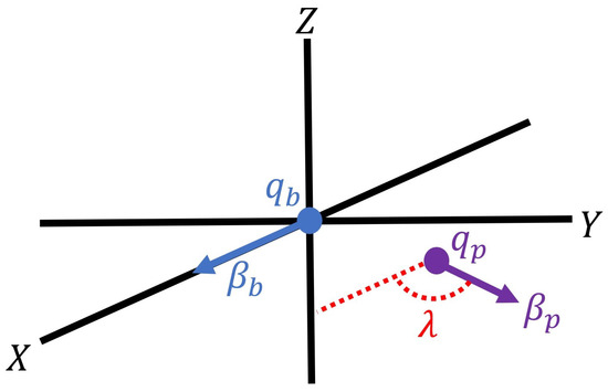
Figure 1.
Charged particles and with their respective velocity vectors.
The force-experiencing particle has an electric field relative to a stationary observer. Its velocity vector is , as shown in Figure 1. In this configuration, the force-experiencing particle will have the (31) electrostatic , aberration and contraction fields.
The additional electric field energy due to overlapping fields can be calculated using Equation (6) applied to the background and particle fields. The electrostatic components of Equations (30) and (31) result in the (32) value of overlapping electrical field energy density.
Integrating the energy density from the right side of Equation (32) will result in the Coulomb law as demonstrated by Equation (6). Therefore, the static field components can be used to describe the classical electrostatic repulsion.
Applying the classical electric field energy density formula to the aberration fields of Equations (30) and (31) results in the (33) value of overlapping electrical field energy density.
Repeating this process for the contraction fields results in Equation (34).
The combined velocity-dependant overlapping energy will be represented by the variable with its volumetric density the sum of Equations (33) and (34) as shown by Equation (35).
For point charges, the contribution of to total energy will equal zero when integrated over a spherical volume and can therefore be removed, as shown in (36).
Equation (36) was calculated by rotating the force-experiencing particle around the z axis. The same result would have been achieved by rotating this particle around any axis perpendicular to motion, provided is defined to be the angle between the two velocity vectors. Therefore, the definition of the dot product as applied to velocity vectors and can be used to express Equation (36) as shown in Equation (37).
Integrating the overlapping energy density as shown in the bracketed term of Equation (37) will result in Coulomb’s law. Therefore, scaling the electrostatic force by the two velocity vectors’ dot product describes the resultant force due to the aberration and contraction fields. This velocity-dependant force will be represented by the vector and is shown in Equation (38), where the charged particles are separated by the vector .
Equation (38) describes a force in the direction of the radius vector pointing from to . Another force due to relativistic effects on these particles can also be derived, as shown in Figure 2.
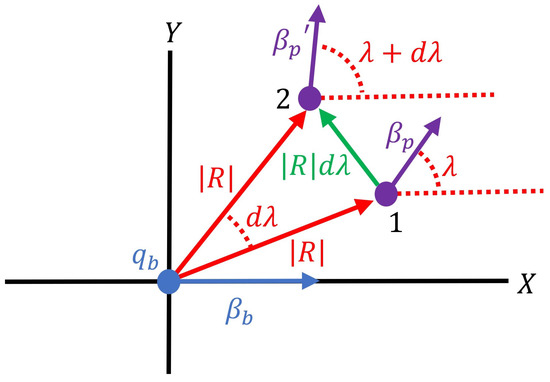
Figure 2.
Charged particles and with rotated around the origin.
Figure 2 depicts a rotation of the force-experiencing particle around the origin. The force described by Equation (38) is perpendicular to this motion and will therefore not result in any momentum change. However, rotating the force-experiencing particle by an angle of around the origin from point 1 to point 2 will cause the velocity vector to change its angle by . This will impact the overlapping electric field energy. Differentiating Equation (36) with respect to the angle as shown in Equation (39) can be used to quantify this effect.
The chain rule can be used to change the (39) derivative to be in terms of distance moved by the force-experiencing particle D where , as shown in Figure 2.
The cross product definition can be used to eliminate from Equation (40). However, care must be taken when applying this substitution to ensure the resultant force is in the displacement vector D direction. The correct direction is achieved by taking the cross product with the normalised radius vector as shown in Equation (41).
Integrating Equation (41) over the electric field volume results in the (42) value of force using the same technique to evaluate Equation (6). Further differentiation is not necessary as Equation (42) has already been differentiated relative to displacement. This velocity-dependant force will be represented by the vector .
Expanding the vector triple product from Equation (42) and adding and together results in the motion-dependant force represented by the variable as shown in Equation (43).
The force described by Equation (43) accounts for all the motion-dependant forces between two charged particles. As such, it will be referred to as the electrodynamic force. The force between two stationary particles can be calculated by integrating the energy described by Equation (32). This force is represented by the vector and referred to as the electrostatic force.
Calculating the total force between two non-accelerating charged particles can be achieved by calculating the electrostatic force , the electrodynamic force and then summing the result. The electrodynamic force is a purely relativistic phenomena as the relativistic aberration of light and Lorentz contractions do not occur in classical physics.
8. Consolidation with Maxwell’s Equations
To demonstrate how this theory applies to to Maxwell’s equations, consider the (45) solution to the magnetic field of a moving particle as derived using Maxwell’s equations. To maintain consistency with existing variables, the magnetic field will be equated to the field-generating particle with electric field of travelling with a velocity of , where .
The force experienced by the force-experiencing particle , with a velocity of , due to the (45) magnetic field can be calculated using the Lorentz force equation to be Equation (46).
The force experienced by the field-generating particle due to this interaction can be calculated using the same analytical process to be Equation (47).
The sum of these magnetic forces does not equal zero. Although Newton’s third law can be violated for relativistic interactions due to the relativity of simultaneity, it is still necessary to demonstrate that the conservation of relativistic momentum in conserved in such cases. This can be demonstrated for two current loops [18] using Jefimenko’s equations. However, Jefimenko’s equations are based on electric current densities and are therefore not explicitly defined for two isolated particles. A more generalised proof is therefore required to demonstrate the compatibility of the electromagnetic interaction with the conservation of momentum.
Applying Equation (43) to the same charged particles results in the (48) value of force-experiencing and field-generating particle force.
The net electrodynamic force described by the (48) interaction equals zero. This is because the electrodynamic force has three force vector components while classical electromagnetic theory only describes two. The vector force components experienced by a charged particle in the radius direction and the other particle’s velocity direction exist in both theories. However, the electrodynamic force also describes a force vector in the direction of a particles own velocity not described by classical electromagnetic theory. This property of the electrodynamic force ensures its compatibility with the conservation of momentum.
Equation (45) also allows the classically defined magnetic field to be equated to the aberration field. This is achieved using the (13) definition of and the aberration component of the (29) background electrodynamic field as described by Equation (49).
Directly related to the aberration field to the magnetic field implies the contraction field has no classical equivalent. To demonstrate why the contraction field has no classical counterpart, consider the electric field due to a line of charge along the x axis in Equation (50) using cartesian coordinates, where is the linear charge density.
The contraction field transformation for (50) will evaluate to zero for motion along the x axis. Therefore, the contraction field cancels out for a continuous flow of charge and is not applicable to situations involving electric current.
The final step in consolidating this theory with Maxwell’s equations is to derive them using the theory presented in this paper. This is achieved by equating the classical electric field to the electrostatic force and the magnetic field to the aberration field. Using these substitutions, it is possible to derive the divergence of both the electric and magnetic field to be equivalent to those defined by Maxwell’s equations.
This result is incompatible with the existence of magnetic monopoles as Gauss’s law for magnetism holds even for single particle fields. Magnetism, as described in this theory, is due to the observed change in photon momentum within an electric field due to motion and does not require magnetic charge.
As demonstrated by the derivation of Equation (49), the (45) relationship between electric and magnetic fields from classical electromagnetism is compatible with this theory. Therefore, taking the divergence of both sides of Equation (45) and using vector identities results in Amperes law.
In Equation (52), will equal zero for all locations within the field where charge is not present. Evaluating this term to a non-zero value requires many particles moving with the same velocity and charge density. In this situation, the electric field divergence will equal its (51) value, allowing Ampere’s magneto-static circuital law to be derived. It is also possible to verify Ampere’s magneto-static circuital law in its integral form from the aberration field by applying Equation (49) to the aberration field of Equation (50).
It is known that magnetism due to circular currents is compatible with the conservation of momentum when accounting for field momentum [18]. It can therefore only be stated that Ampere’s magneto-static circuital law is valid for applications involving electric current. In this application, the electrodynamic force component in the force-experiencing particle’s velocity direction will cancel out, resulting in the same value predicted by the Lorentz force equation. Therefore, combining Ampere’s magneto-static circuital law and the Lorentz force equation are special cases of a more generalised electromagnetic interaction that is not usually encountered. Maxwell’s addition to Ampere’s law as derived in Equation (52) is unaffected by charge distribution and is therefore universally compatible with this theory.
Deriving Faraday’s law from inertial frame transformations is difficult, as the change in magnetic field densities observed relative to a non-accelerating charged particle should be zero. This will result in Faraday’s law evaluating to 0. However, an electromagnetic wave can be observed from different inertial frames. Observers may disagree on the waves frequency and direction, but should agree that it is a wave travelling at the speed of light. Therefore, Equation (53) should be valid for all observers.
The left hand side of Equation (53) can be derived by taking the negative curl of the electric field curl using the vector identity as shown by Equation (54). The term evaluates to zero for an electromagnetic wave, as charge densities within the wave are zero.
The right hand side of Equation (53) can be derived by taking the partial time derivative of Equation (52), resulting in Equation (55) when .
Substituting the (54) electric field vector Laplacian and the (55) second-order electric field partial time derivative into Equation (53) results in Faraday’s law as shown in Equation (56).
Another aspect of electromagnetic theory that can be reconciled with special relativity is that of energy. The electrodynamic force, as described in this paper, was derived by scaling electromagnetic energy due to motion by . As such, it is compatible with electric field energy contributing to a particle’s mass as was theorised by physicists in the early 20th century.
It has also been assumed that the one-way speed of light is the same as its two-way speed in this analysis. If this is not the case, the aberration angle would differ based on particle orientation. This difference would not be measurable for a single particle due to the clock synchronisation effects of special relativity. However, the speed of light in both directions along perpendicular to motion axes is required to be known at the same observed time and location to calculate overlapping field energy. Light speed asymmetries would not change the electrostatic force, although it would impact the electrodynamic force. As both the fine structure constant and anomalous magnetic moment are known to high precision [19], any light speed asymmetries are likely to be minute or non-existent according to this theory.
9. Conclusions
This paper has demonstrated an analytical technique whereby electromagnetic energy can be transformed between inertial frames in a way that is directly compatible with special relativity. This also ensures the classical electromagnetic interaction between two isolated particles is compatible with the conservation of momentum.
This analytical technique demonstrates how the Lorentz contractions gives rise to electromagnetic energy that is currently unaccounted for. When magnetic fields are due to a continuous flow of charge, this energy has no impact on the resultant magnetic field. Not satisfying this criteria, such as occurs in isolated particle interactions, has implications for the use of Ampere’s magneto-static circuital law and the Lorentz force equation.
Further implications of this analysis apply to conjecture relating to magnetic charge, as such a concept is incompatible with this theory. Magnetism is entirely due to observer velocity-dependant changes in photon momentum and does not require the existence of magnetic monopoles. This paper also establishes a theoretical basis for continued discussion regarding the electromagnetic contribution to a particle’s mass and the implications of light speed asymmetries.
Funding
This research was funded through the provision of an Australian Government Research Training Program Scholarship, a Monash University Faculty of Information Technology Research Scholarship and a CSIRO Data61 Scholarship.
Conflicts of Interest
The author declares no conflict of interest. The funders had no role in the design of the study; in the collection, analyses, or interpretation of data; in the writing of the manuscript, or in the decision to publish the results.
References
- Herr, W. Short theory of special relativity and invariant formulation of electrodynamics. CERN Yellow Rep. Sch. Proc. 2018, 1, 27. [Google Scholar]
- Thomson, J. On the electric and magnetic effects produced by the motion of electrified bodies. Lond. Philos. Mag. J. Sci. 1881, 5, 11–68. [Google Scholar] [CrossRef]
- Heaviside, O. On the electromagnetic effects due to the motion of electrification through a dielectric. Lond. Edinb. Dublin Philos. Mag. J. Sci. 1889, 27, 324–339. [Google Scholar] [CrossRef]
- Jantzen, R.T.; Ruffini, R. Fermi and electromagnetic mass. Gen. Relativ. Gravit. 2012, 44, 2063–2076. [Google Scholar] [CrossRef]
- Mamone Capria, M.; Manini, M.G. On the relativistic unification of electricity and magnetism. arXiv 2011, arXiv:1111.7126. [Google Scholar]
- Hassani, M. Special Relativity: A Heuristic Approach; Elsevier: Amsterdam, The Netherlands, 2017; pp. 117–136. [Google Scholar]
- Rosser, W.G.V. Classical Electromagnetism via Relativity: An Alternative Approach to Maxwell’s Equations; Springer: Berlin/Heidelberg, Germany, 2013. [Google Scholar]
- Smith, G.S. Visualizing special relativity: The field of an electric dipole moving at relativistic speed. Eur. J. Phys. 2011, 32, 695. [Google Scholar] [CrossRef]
- Mansuripur, M. The force law of classical electrodynamics: Lorentz versus Einstein and Laub. Opt. Trapp. Opt. Micromanip. X 2013, 8810, 88100K. [Google Scholar]
- Johns, O.D. Relativistically Correct Electromagnetic Energy Flow. arXiv 2020, arXiv:2010.10263. [Google Scholar]
- Mansuripur, M. Trouble with the Lorentz law of force: Incompatibility with special relativity and momentum conservation. Phys. Rev. Lett. 2012, 108, 193901. [Google Scholar] [CrossRef] [PubMed]
- Kholmetskii, A.L.; Missevitch, O.V.; Yarman, T. Force law in material media, hidden momentum and quantum phases. Ann. Phys. 2016, 369, 139–160. [Google Scholar] [CrossRef]
- Stachel, J.J.; Cassidy, D.C.; Renn, J.; Schulmann, R. Einstein and Laub on the electrodynamics of moving media. Collect. Pap. Albert Einstein 1989, 2, 1900–1909. [Google Scholar]
- McDonald, K.T. (Princeton University, Princeton, NJ, USA). Biot-Savart vs. Einstein-Laub Force Law. 2013. Available online: https://www.physics.princeton.edu/~mcdonald/examples/laub.pdf (accessed on 8 November 2021).
- Shockley, W.; James, R.P. “Try Simplest Cases” Discovery of “Hidden Momentum” Forces on “Magnetic Currents”. Phys. Rev. Lett. 1967, 18, 876–879. [Google Scholar] [CrossRef]
- Mansuripur, M. The Lorentz Force Law and Its Connections to Hidden Momentum, the Einstein-Laub Force, and the Aharonov-Casher Effect. IEEE Trans. Magn. 2014, 50, 1–10. [Google Scholar] [CrossRef][Green Version]
- Buonaura, B.; Giuliani, G. Wave and photon descriptions of light: Historical highlights, epistemological aspects and teaching practices. Eur. J. Phys. 2016, 37, 055303. [Google Scholar] [CrossRef]
- Tuval, M.; Yahalom, A. Newton’s third law in the framework of special relativity. Eur. Phys. J. Plus 2014, 129, 1–8. [Google Scholar] [CrossRef]
- Morel, L.; Yao, Z.; Clade, P.; Guellati-Khelifa, S. Determination of the fine-structure constant with an accuracy of 81 parts per trillion. Nature 2020, 588, 61–65. [Google Scholar] [CrossRef] [PubMed]
Publisher’s Note: MDPI stays neutral with regard to jurisdictional claims in published maps and institutional affiliations. |
© 2022 by the author. Licensee MDPI, Basel, Switzerland. This article is an open access article distributed under the terms and conditions of the Creative Commons Attribution (CC BY) license (https://creativecommons.org/licenses/by/4.0/).