Variational Principles for Double-Layer Graphene Nanoribbons Undergoing Vibrations Including Shear and Tensile–Compressive Effects

Abstract

Variational principles and variationally consistent boundary conditions are presented for double-layer graphene nanoribbons undergoing time-dependent and free vibrations. The van der Waals forces acting in the core region are modelled as shear and tensile–compressive effects. The nonlocal constitutive formulation of the problem is based on the sandwich beam model in order to represent the graphene nanoribbon layers as faces and van der Waals forces acting in the core region. The constitutive equations which govern the vibrations of the nanoribbons are in the form of four coupled partial differential equations involving the in-plane and out-of-plane deflections. The first part of the study involves the derivation of the variational principle for the system undergoing time-dependent vibrations. Hamilton’s principle is formulated based on the kinetic and potential energies of the system. The next section involves the freely vibrating nanoribbon system and the formulation of the variational principle for this case is given. Based on this formulation, the expressions for the Rayleigh quotients are obtained for the longitudinal natural frequency and the transverse natural frequency. The last section involves the derivation of the variationally consistent boundary conditions and the expressions for the shear force and moment at the boundaries.

1. Introduction

Graphene nanoribbons (GNRs) are narrow strips of graphene with a width of about 50 nm or less and can be classified as armchair GNRs, zigzag GNRs, and chiral GNRs based on the edge geometry as noted in [1]. It was noted in [2] that elastic properties of GNRs depend on their width. Their unique properties come into use in a wide range of applications in electronics and in a number of other fields. Presently they are part of a large number of carbon-based applications due to their unique and versatile properties as noted in [3]. The properties and the applications of GNRs have been the subject of several review articles. Magnetic, electronic and optical properties of GNRs have been discussed in [4] which also provided extensive information on several areas of applications of GNRs.

A detailed study of the properties of GNRs, as well as the fabrication methods, is given in [5]. This is followed by a discussion of the areas of applications of GNRs as well as information on their electronic, electromagnetic, thermal and optical properties. Lou et al. [1] note that an outstanding feature of GNRs is their electronic properties which are used extensively in nanoelectronic applications as reviewed in [6]. These properties allow GNRs to have applications in such diverse areas as transistors, sensors, and quantum dots, which are semiconductor components with unique optical and electronic properties [7]. The width and edge configurations of GNRs can be adjusted to fine-tune their electronic properties to create semiconducting properties as noted in [8].

Flexibility in tuning the electronic properties of GNRs makes them a versatile material in a number of fields. Different properties of GNRs have been the subject of a number of articles which include [9] on electronic properties, and [10,11] on photoelectric and optoelectronic properties. These publications also discussed the other areas of applications of GNRs based on their electronic properties. One area where GNRs can be employed is for their use as transistors as noted in [12,13]. A recent study by Radsar et al. [14] noted their use as field effect transistors. Another area of application of GNRs is quantum electronics as noted in [15,16]. An important area of application of GNRs is the medical field where they are used as DNA sensors [17] and for DNA sequencing [18]. Biomedicine is another area of application of GNRs as discussed in the articles [19,20,21]. GNR applications in this area include biosensing [22,23] and their use as cancer biomarkers as shown in [24], which names GNRs as a cutting-edge material for this purpose. Further applications of GNRs in the biomedical field have been discussed in [25] with state-of-the art applications of GNRs in health care presented in [26]. A recent application of graphene involves nanomechanical resonators which use multiple graphene layers to convert digital video signals to modulated vibrations as presented in [27]. The ongoing research on photonic nanomembranes with van der Waals interfaces was reviewed in [28]. It was noted in [28] that these nanomembranes are ultrathin and as such they can be used to design light photonic devices which can be used in health-care applications.

An extension of single-layer GNRs is double-layer graphene nanoribbons (DLGNRs). DLGNRs are made of two layers of nanoribbons which are held together by van der Waals forces. Vibrations of DLGNRs involving in-phase and anti-phase modes were studied by Shi et al. [29]. It was noted that vibrational properties of DLGNRs differ in in-phase and anti-phase modes. An important consideration in the bending of multilayer GNRs is the interlayer shear effect which has been studied in [30] in the case of the bending of bilayer and triple-layer GNRs. It was noted that in-plane displacements of GNRs can have a significant effect on the bending of multilayer GNRs. The interlayer shear effect on the vibrations of DLGNRs has been studied in [31] which also included the effect of the tensile–compressive forces on the vibrations. A further study on the interlayer shear effect between GNRs and the elastic medium and its influence on the vibrations of DLGNRs includes reference [32]. In [32], the governing equations were based on the sandwich beam model.

A further extension of DLGNRs is multilayer GNRs (MLGNRs). Vibrations of MLGNRs have been studied in a number of articles. A molecular dynamics approach was implemented in [33,34] to study the interlayer shear effect of van der Waals forces on the vibrations of MLGNRs. Further studies on the shear effect of van der Waals interactions on the vibrations of MLGNRs include [35] where a nonlocal Timoshenko beam model was implemented.

Vibrations of DLGNRs were studied in [36] with GNRs modelled as sandwich beams and taking into account the tensile, compressive and interlayer shear effects of van der Waal forces between the layers of GNRs. It was observed that the tensile–compressive effects of the interlayer on the frequencies are higher as compared to the shear effects, especially at higher modes. Results are given for the first five frequencies and for the clamped–clamped boundary conditions. Vibrations of multilayer GNRs taking the interlayer shear effect into account were studied in [37] based on the Reddy beam model. The finite element method was used to study the buckling of DLGNRs in [38] with the results given for different types of chirality and stacking sequences. The continuum model was used to study the buckling of DLGNRs in [39] based on the nonlocal elasticity theory. A review of the implementation of nonlocal elastic models to study the mechanics of nanoscale components such as carbon nanotubes and graphene sheets is given in [40].

In the present study, variational formulations are given for double-layer graphene nanoribbons for two cases, namely for DLGNRs undergoing time-dependent vibrations and for DLGNRs undergoing free vibrations. The core region between the top and bottom nanoribbons is subject to van der Waals forces. Constitutive equations for the core region include the interlayer tensile–compressive forces and the shear effect of van der Waals forces. A variational formulation is used to formulate Hamilton’s principle for the present case. This is followed by the variational formulation for the case involving the freely vibrating DLGNRs. Based on this formulation, expressions for the longitudinal and transverse natural frequencies are given as Rayleigh quotients which provide a qualitative assessment of the effect of various problem parameters on vibration frequencies. The last part of the paper involves the derivations of the boundary conditions for the freely vibrating DLGNRs and the expressions for the shear force and the moment expressions at the supports.

An extensive study of the variational principles of nonlocal elasticity was the subject of a paper by Polizzotto [41]. A variational formulation for nonlocal beams subject to torsion was given in [42] which included variationally consistent boundary conditions. Recent results on the variational principles involving the vibrations of nanoscale components include [43] on the coupled carbon nanotubes subject to a magnetic field and [44] on the coupled Boron Nitride nanotubes subject to piezoelastic and surface effects. The present study extends these results to double-layer graphene nanoribbons for time-dependent and free vibration cases and includes the expressions for variationally consistent boundary conditions.

2. Physical Problem

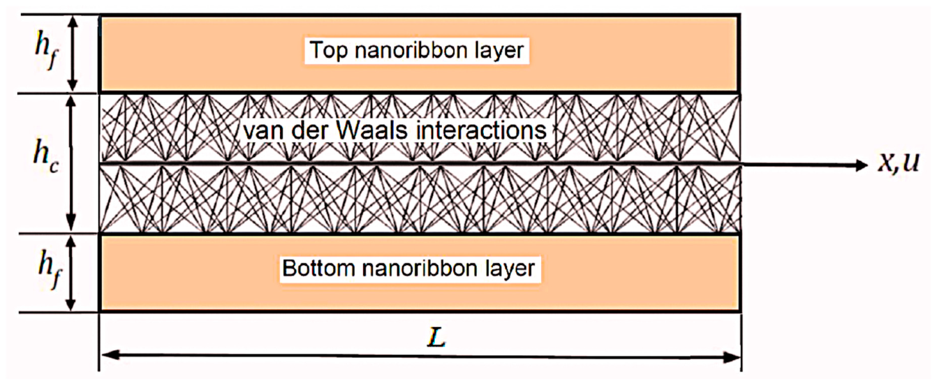
Each nanoribbon of the double GNR system is defined as a Euler–Bernoulli beam with constitutive modelling based on the nonlocal elasticity theory. Interactions between the nanoribbons are due to van der Waals forces between the nanoribbons as shown in Figure 1. Constitutive modelling of the interlayer between the nanotubes includes shear and tensile–compressive effects and is based on the nonlocal elasticity theory which is detailed in [45].

A double-layer graphene nanoribbon of length $L$ is shown in Figure 1. The origin of the Cartesian coordinate system shown in Figure 1 is located at the left-hand side of the beam and in the middle of the core section. In Figure 1, the length of the GNR is denoted by $L$. Each nanoribbon is modelled as a nonlocal Euler–Bernoulli beam. The thickness of the core section of GNRs between the top and bottom nanoribbons is denoted as $h_c$ and the thickness of each top and bottom nanoribbon layer is denoted as $h_f$. The $x$ coordinate is located in the middle of the double GNR system as shown in Figure 1 with the origin of the coordinate system located on the left end of the nanoribbon system. Displacements of GNRs in the longitudinal direction are given by $u_1\left(x,t\right)$ and $u_2\left(x,t\right)$ and in the transverse direction by $w_1\left(x,t\right)$ and $w_2\left(x,t\right)$, with indices 1 and 2 referring to the top and bottom GNRs, respectively. The differential equations governing the nonlocal vibrations of the double GNR system are given in [31]:

$$D_1\left(u_1,u_2,w_1, w_2\right)=J\left(u_1\right)+K_1\left(u_1-u_2\right)+L\left(w_1, w_2 \right)=0$$

(1)

$$D_2\left(u_1,u_2,w_1, w_2\right)=J\left(u_2 \right)-K_1\left(u_1-u_2\right)-L\left(w_1, w_2 \right)=0$$

(2)

$$D_3\left({u_1, u}_2,w_1,w_2\right)=M\left(w_1\right)+N_1\left(w_1,w_2 \right)-N_2\left(w_1,w_2 \right)+K_2\left(u_1,u_2\right)=0$$

(3)

$$D_4\left({u_1, u}_2,w_1,w_2\right)=M\left(w_2\right)-N_1\left(w_1,w_2 \right)-N_2\left(w_1,w_2 \right)+K_2\left(u_1,u_2\right)=0$$

(4)

where

$$J\left(u_i\right)=-E_f{A}_f{\displaystyle \frac{{\mathsf{\partial }}^2{u}_i}{\mathsf{\partial }{x}^2}}+\rho A_f{\displaystyle \frac{{\mathsf{\partial }}^2{u}_i}{\mathsf{\partial }{t}^2}}-\mu \rho A_f{\displaystyle \frac{{\mathsf{\partial }}^4{u}_i}{\mathsf{\partial }{x}^2\mathsf{\partial }{t}^2}}$$

(5)

$$K_1\left(u_1-u_2\right)={\displaystyle \frac{G_c{A}_c}{h_c^2}}\left(u_1-u_2\right)$$

(6)

$$K_2\left(u_1,u_2\right)={\displaystyle \frac{G_c{A}_c(h_f+h_c)}{2h_c^2}}\left({\displaystyle \frac{\mathsf{\partial }{u}_2}{\mathsf{\partial }x}}-{\displaystyle \frac{\mathsf{\partial }{u}_1}{\mathsf{\partial }x}}\right)$$

(7)

$$L\left(w_1, w_2 \right)={\displaystyle \frac{G_c{A}_c\left(h_f+h_c\right)}{2h_c^2}}\times \left({\displaystyle \frac{\mathsf{\partial }{w}_1}{\mathsf{\partial }x}}+{\displaystyle \frac{\mathsf{\partial }{w}_2}{\mathsf{\partial }x}}\right)$$

(8)

$$M\left(w_i \right)=E_f{I}_f{\displaystyle \frac{{\mathsf{\partial }}^4{w}_i}{\mathsf{\partial }{x}^4}}+\rho A_f{\displaystyle \frac{{\mathsf{\partial }}^2{w}_i}{\mathsf{\partial }{t}^2}}-\mu \rho A_f{\displaystyle \frac{{\mathsf{\partial }}^4{w}_i}{\mathsf{\partial }{x}^2\mathsf{\partial }{t}^2}}$$

(9)

$$N_1\left(w_1,w_2 \right)=-{\displaystyle \frac{G_c{I}_c}{h_c^2}}\times \left({\displaystyle \frac{{\mathsf{\partial }}^2{w}_1}{\mathsf{\partial }{x}^2}}-{\displaystyle \frac{{\mathsf{\partial }}^2{w}_2}{\mathsf{\partial }{x}^2}}\right)+{\displaystyle \frac{E_c{A}_c}{h_c^2}}\left(w_1-w_2\right)$$

(10)

$$N_2\left(w_1,w_2 \right)={\displaystyle \frac{G_c{A}_c{\left(h_f+h_c\right)}^2}{4h_c^2}}\times \left({\displaystyle \frac{{\mathsf{\partial }}^2{w}_1}{\mathsf{\partial }{x}^2}}+{\displaystyle \frac{{\mathsf{\partial }}^2{w}_2}{\mathsf{\partial }{x}^2}}\right)$$

(11)

The nonlocal parameter $\mu ={\left(e_{0}a\right)}^2$ in Equations (5) and (9) is a length scale which depends on a number of factors. These factors include the chirality of GNRs, number of layers and the boundary conditions as noted in [31]. In Equations (5) and (6), $E_f$ is the Young modulus of the GNRs, and $G_c$ is the shear modulus of the core section. The cross-sectional areas of the GNRs and the core sections are denoted as $A_f$ and $A_c$, respectively, with $\rho$ denoting the density of the GNRs. The second moments of the GNRs and the core area are denoted as $I_f$ and $I_c$, respectively. The time domain of the vibrations is defined as $t_1\le t\le t_2$. The accuracy of the formulation for the double-layer graphene nanoribbons as given by Equations (1)–(4) and the solution method implemented in [31] have been verified in [31]. Verification involved the comparison of the frequencies obtained based on the constitutive modelling presented in [31] with the numerical results given in references [30,34,36]. The comparisons indicated a high level of accuracy of the present formulation and the numerical results obtained in [31] involving the vibrations of double-layer GNRs.

3. Variational Formulation

In the present section, the variational formulation for the DLGNRs is presented with the DLGNRs undergoing time-dependent vibrations. The variational principle for the system of differential Equations (1)–(4) is derived by introducing the functionals $V_i\left(u_i\right), { V}_i\left(w_i\right), i=1,2$, $V_3\left(u_1-u_2,w_1,w_2\right)$ and $V_4\left(w_1,w_2\right)$. The variational expression for the present problem is denoted as $V\left({u_1, u_2, w}_1,w_2\right)$ and is given in terms of $V_i\left(u_i\right), { V}_i\left(w_i\right), V_3\left(u_1-u_2,w_1,w_2\right)$ and $V_4\left(w_1,w_2\right)$ as

$$V\left({u_1, u_2, w}_1,w_2\right)={\displaystyle \sum _{i=1}^2}{V}_i\left(u_i\right)+{\displaystyle \sum _{i=1}^2}{V}_i\left(w_i\right)+V_3\left(u_1-u_2,w_1,w_2\right)+V_4\left(w_1,w_2\right)$$

(12)

In Equation (12), the functional $V\left({u_1, u_2, w}_1,w_2\right)$ is expressed in terms of a number of functionals which are to be determined next. Variational functionals involving only $u_i$ and $w_i$ are given by $V_i\left(u_i\right)$ and $V_i\left(w_i\right)$ which are defined as follows:

$$V_i\left(u_i\right)={\displaystyle \frac{1}{2}}{\int }_{t_1}^{t_2}{\int }_0^L\left[{E_{f}A}_f{\left({\displaystyle \frac{\mathsf{\partial }{u}_i}{\mathsf{\partial }x}}\right)}^2-\rho A_f{\left({\displaystyle \frac{\mathsf{\partial }{u}_i}{\mathsf{\partial }t}}\right)}^2-\mu \rho A_f{\left({\displaystyle \frac{{\mathsf{\partial }}^2{u}_i}{\mathsf{\partial }x\mathsf{\partial }t}}\right)}^2\right]dx dt, i=1,2$$

(13)

$$V_i\left(w_i\right)={\displaystyle \frac{1}{2}}{\int }_{t_1}^{t_2}{\int }_0^L\left[E_f{I}_f{\left({\displaystyle \frac{{\mathsf{\partial }}^2{w}_i}{\mathsf{\partial }{x}^2}}\right)}^2-\rho A_f{\left({\displaystyle \frac{\mathsf{\partial }{w}_i}{\mathsf{\partial }t}}\right)}^2-\mu \rho A_f{\left({\displaystyle \frac{{\mathsf{\partial }}^2{w}_i}{\mathsf{\partial }x\mathsf{\partial }t}}\right)}^2\right]dx dt, i=1,2$$

(14)

The expression for $V_3\left(u_1-u_2,w_1,w_2\right)$ is given by

$$V_3\left(u_1-u_2,w_1,w_2\right)={\displaystyle \frac{1}{2}}{\int }_{t_1}^{t_2}{\int }_0^L\left[\left({\displaystyle \frac{G_c{A}_c}{2h_c^2}}\right){\left(u_1-u_2\right)}^2+{\displaystyle \frac{G_c{A}_c\left(h_f+h_c\right)}{h_c^2}}\times \left(u_1-u_2\right)\times \left({\displaystyle \frac{\mathsf{\partial }{w}_1}{\mathsf{\partial }x}}+{\displaystyle \frac{\mathsf{\partial }{w}_2}{\mathsf{\partial }x}}\right)\right]dx dt$$

(15)

The variational functional $V_4\left(w_1,w_2\right)$ with both the functions $w_1$ and $w_2$ is defined as

$$V_4\left(w_1,w_2\right)={\displaystyle \frac{1}{2}}{\int }_{t_1}^{t_2}{\int }_0^L\left[{\displaystyle \frac{G_c{I}_c}{2h_c^2}}{\left({\displaystyle \frac{\mathsf{\partial }{w}_1}{\mathsf{\partial }x}}-{\displaystyle \frac{\mathsf{\partial }{w}_2}{\mathsf{\partial }x}}\right)}^2+{\displaystyle \frac{E_c{A}_c}{{2h}_c^2}}{\left(w_1-w_2\right)}^2+{\displaystyle \frac{G_c{A}_c{\left(h_f+h_c\right)}^2}{4h_c^2}}\times {\left({\displaystyle \frac{\mathsf{\partial }{w}_1}{\mathsf{\partial }x}}+{\displaystyle \frac{\mathsf{\partial }{w}_2}{\mathsf{\partial }x}}\right)}^2\right]dx dt$$

(16)

The Euler–Lagrange equations of the functionals $V_i\left(u_i\right)$ in Equation (13) and $V_i\left(w_i\right)$ in Equation (14) correspond to the differential expressions $J\left(u_i\right)$ in Equation (5) and $M\left(w_i\right)$ in Equation (9), respectively. Similarly, the Euler–Lagrange equations of the functional $V_3\left(u_1-u_2,w_1,w_2\right)$ in Equation (15) and the functional $V_4\left(w_1,w_2\right)$ in Equation (16) correspond to the differential expressions in Equations (6)–(8) and Equations (10) and (11). As such, the differential equations in Equations (1)–(4) correspond to the Euler–Lagrange equations of the functional $V\left({u_1, u_2, w}_1,w_2\right)$ in Equation (12). This constitutes the variational formulation of the double-layer GNRs in the case of time-dependent vibrations.

4. Hamilton’s Principle

Hamilton’s principle is used extensively in continuum mechanics and, in particular, for the derivation of differential equations governing the mechanics of beams, plates and shells as noted in [34,35]. It also allows for the formulation of analytical and numerical approximations for the solution of a large number of mechanics problems. A detailed study of Hamilton’s principle is given in the book by Bedford [46] and in an article [47]. A study of Hamilton’s principle in dynamical problems is given in [48]. In the present case, Hamilton’s principle is given by

$${\int }_{t_1}^{t_2}\left[\delta KE\left(t\right)-\left(\delta {PE}_1\left(t\right)+\delta {PE}_2\left(t\right)\right)\right]dt=0$$

(17)

Functionals $KE\left(t\right)$, ${PE}_1\left(t\right)$ and ${PE}_2\left(t\right)$ in Equation (17) are defined as follows:

$$KE\left(t\right)={\displaystyle \frac{1}{2}}{\displaystyle \sum _{i=1}^2}{\int }_0^L\left[-\rho A_f{\left({\displaystyle \frac{\mathsf{\partial }{u}_i}{\mathsf{\partial }t}}\right)}^2-\mu \rho A_f{\left({\displaystyle \frac{{\mathsf{\partial }}^2{u}_i}{\mathsf{\partial }x\mathsf{\partial }t}}\right)}^2-\rho A_f{\left({\displaystyle \frac{\mathsf{\partial }{w}_i}{\mathsf{\partial }t}}\right)}^2-\mu \rho A_f{\left({\displaystyle \frac{{\mathsf{\partial }}^2{w}_i}{\mathsf{\partial }x\mathsf{\partial }t}}\right)}^2\right]dx$$

(18)

$${PE}_1\left(t\right)={\displaystyle \frac{1}{2}}{\displaystyle \sum _{i=1}^2}{\int }_0^L\left[E_f{A}_f{\left({\displaystyle \frac{\mathsf{\partial }{u}_i}{\mathsf{\partial }x}}\right)}^2+E_f{I}_f{\left({\displaystyle \frac{{\mathsf{\partial }}^2{w}_i}{\mathsf{\partial }{x}^2}}\right)}^2+\left[\left({\displaystyle \frac{G_c{A}_c}{2h_c^2}}\right){\left(\Delta u_{12}\right)}^2+{\displaystyle \frac{G_c{A}_c\left(h_f+h_c\right)}{h_c^2}}\Delta u_{12}\times \left({\displaystyle \frac{\mathsf{\partial }{w}_1}{\mathsf{\partial }x}}+{\displaystyle \frac{\mathsf{\partial }{w}_2}{\mathsf{\partial }x}}\right)\right]\right]dx$$

(19)

$${PE}_2\left(t\right)={\int }_0^L\left[{\displaystyle \frac{G_c{I}_c}{2h_c^2}}{\left({\displaystyle \frac{\mathsf{\partial }\Delta w_{12}}{\mathsf{\partial }x}}\right)}^2+{\displaystyle \frac{E_c{A}_c}{{2h}_c^2}}{\left(\Delta w_{12}\right)}^2+{\displaystyle \frac{G_c{A}_c{\left(h_f+h_c\right)}^2}{4h_c^2}}\times {\left({\displaystyle \frac{\mathsf{\partial }{w}_1}{\mathsf{\partial }x}}+{\displaystyle \frac{\mathsf{\partial }{w}_2}{\mathsf{\partial }x}}\right)}^2\right]dx$$

(20)

where $\Delta u_{12}=u_1-u_2$ and $\Delta w_{12}=w_1-w_2$. In Equations (18)–(20), $KE\left(t\right)$ is the kinetic energy, and ${PE}_i\left(t\right)$, $i=1,2$, is the potential energy of deformation.

5. Variational Principles for Nanoribbons Undergoing Free Vibrations

In the present section, a variational formulation for the time-independent case involving the free vibrations of the double-layer graphene nanoribbons is presented. In the case of a freely vibrating double-layered GNR system, the deflection functions in the longitudinal and transverse directions are given by

$$u_i\left(x,t\right)=U_i{\left(x\right) e}^{i\overline{\omega }t}$$

(21)

$$w_i\left(x,t\right)=W_i{\left(x\right) e}^{i\omega t}$$

(22)

where $\overline{\omega }$ is the longitudinal natural frequency of $u_i\left(x,t\right)$ and $\omega$ is the transverse natural frequency of $w_i\left(x,t\right)$, $i=1,2$. Governing equations for the case of free vibrations can be obtained by substituting Equations (21) and (22) for $u_i\left(x,t\right)$ and $w_i\left(x,t\right)$ into constitutive Equations (1)–(4). This operation gives the equations governing the free vibrations of the double-layered GNR system as follows:

$$D_{FV1}\left(U_1,U_2,W_1, W_2\right)=J_{FV}\left(U_1\right)+K_{FV1}\left(U_1-U_2\right)+L_{FV}\left(W_1, W_2 \right)=0$$

(23)

$$D_{FV2}\left(U_1,U_2,W_1, W_2\right)=J_{FV}\left(U_2\right)-K_{FV1}\left(U_1-U_2\right)-L_{FV}\left(W_1, W_2 \right)=0$$

(24)

$$D_{FV3}\left(U_1,U_2,W_1, W_2\right)=M_{FV}\left(W_1\right)+N_{FV1}\left(W_1,W_2 \right)-N_{FV2}\left(W_1,W_2 \right)+K_{FV2}\left(U_1,U_2\right)=0$$

(25)

$$D_{FV4}\left(U_1,U_2,W_1, W_2\right)=M_{FV}\left(W_2\right)-N_{FV1}\left(W_1,W_2 \right)-N_{FV2}\left(W_1,W_2 \right)+K_{FV2}\left(U_1,U_2\right)=0$$

(26)

where the differential operators $J_{FV}\left(U_i\right)$, $M_{FV}\left(W_i\right)$, $N_{FVi}\left(W_1,W_2 \right)$, $i=1,2$; $L_{FV}\left(W_1, W_2 \right)$, $K_{FV1}\left(U_1-U_2\right)$ and $K_{FV2}\left(U_1,U_2\right)$ are defined as follows:

$$J_{FV}\left(U_i\right)=-E_f{A}_f{\displaystyle \frac{d^2{U}_i}{d{x}^2}}-\rho A_f{\overline{\omega }}^2{U}_i+\mu {\overline{\omega }}^2\rho A_f{\displaystyle \frac{d^2{U}_i}{d{x}^2}}$$

(27)

$$K_{FV1}\left(U_1-U_2\right)={\displaystyle \frac{G_c{A}_c}{h_c^2}}\left(U_1-U_2\right)$$

(28)

$$L_{FV}\left(W_1, W_2 \right)={\displaystyle \frac{G_c{A}_c\left(h_f+h_c\right)}{2h_c^2}}\times \left({\displaystyle \frac{d{W}_1}{dx}}+{\displaystyle \frac{d{W}_2}{dx}}\right)$$

(29)

$$M_{FV}\left(W_i\right)=E_f{I}_f{\displaystyle \frac{d^4{W}_i}{d{x}^4}}-{\omega }^2\rho A_f{W}_i+{\omega }^2\mu \rho A_f{\displaystyle \frac{d^2{W}_i}{d{x}^2}}$$

(30)

$$N_{FV1}\left(W_1,W_2 \right)=-{\displaystyle \frac{G_c{I}_c}{h_c^2}}\times \left({\displaystyle \frac{d^2{W}_1}{d{x}^2}}-{\displaystyle \frac{d^2{W}_2}{d{x}^2}}\right)+{\displaystyle \frac{E_c{A}_c}{h_c^2}}\left(W_1-W_2\right)$$

(31)

$$N_{FV2}\left(W_1,W_2 \right)={\displaystyle \frac{G_c{A}_c{\left(h_f+h_c\right)}^2}{4h_c^2}}\times \left({\displaystyle \frac{d^2{W}_1}{d{x}^2}}+{\displaystyle \frac{d^2{W}_2}{d{x}^2}}\right)$$

(32)

$$K_{FV2}\left(U_1,U_2\right)={\displaystyle \frac{G_c{A}_c(h_f+h_c)}{2h_c^2}}\left({\displaystyle \frac{d{U}_2}{dx}}-{\displaystyle \frac{d{U}_1}{dx}}\right)$$

(33)

For the case of a freely vibrating double-layered GNR system, the variational expression is given by

$$V_{FV}\left({U_1, U_2, W}_1,W_2\right)={\displaystyle \sum _{i=1}^2}{V}_{FV1}\left(U_i\right)+{\displaystyle \sum _{i=1}^2}{V}_{FV2}\left(W_i\right)+V_{FV3}\left(U_1-U_2,W_1,W_2\right)+V_{FV4}\left(W_1,W_2\right)$$

(34)

Expression (34) gives the variational formulation for the freely vibrating double-layered GNR system. Governing constitutive Equations (23)–(26) for this case correspond to the Euler–Lagrange equations of Equation (34). The variational functional $V_{FVi}\left(U_i\right)$ in Equation (34) is given by

$$V_{FVi}\left(U_i\right)={\displaystyle \frac{1}{2}}{\int }_0^L\left[E_f{A}_f{\left({\displaystyle \frac{d{U}_i}{dx}}\right)}^2-{\overline{\omega }}^2\rho A_f{U}_i^2-\mu {\overline{\omega }}^2\rho A_f{\left({\displaystyle \frac{d{U}_i}{dx}}\right)}^2\right]dx, i=1,2$$

(35)

where $i=1,2$. The variational functional $V_{FV2}\left(W_i\right)$ is given by

$$V_{FVi}\left(W_i\right)={\displaystyle \frac{1}{2}}{\int }_0^L\left[E_f{I}_f{\left({\displaystyle \frac{d^2{W}_i}{d{x}^2}}\right)}^2-{\omega }^2\rho A_f{W_i}^2-\mu {\omega }^2\rho A_f{\left({\displaystyle \frac{d{W}_i}{dx}}\right)}^2\right]dx, i=1,2$$

(36)

Variational functionals $V_{FV3}\left(U_1-U_2,W_1,W_2\right)$ and $V_{VF4}\left(W_1,W_2\right)$ are defined as

$$V_{VF3}\left(U_1-U_2,W_1,W_2\right)={\displaystyle \frac{1}{2}}{\int }_0^L\left[\left({\displaystyle \frac{G_c{A}_c}{2h_c^2}}\right){\left(U_1-U_2\right)}^2+{\displaystyle \frac{G_c{A}_c\left(h_f+h_c\right)}{h_c^2}}\times \left(U_1-U_2\right)\times \left({\displaystyle \frac{d{W}_1}{dx}}+{\displaystyle \frac{d{W}_2}{dx}}\right)\right]dx$$

(37)

$$V_{VF4}\left(W_1,W_2\right)={\displaystyle \frac{1}{2}}{\int }_0^L\left[{\displaystyle \frac{G_c{I}_c}{2h_c^2}}\left[{\left({\displaystyle \frac{d^2{W}_1}{d{x}^2}}\right)}^2-{\left({\displaystyle \frac{d^2{W}_2}{d{x}^2}}\right)}^2\right]+{\displaystyle \frac{E_c{A}_c}{{2h}_c^2}}{\left(W_1-W_2\right)}^2-{\displaystyle \frac{G_c{A}_c{\left(h_f+h_c\right)}^2}{4h_c^2}}\left[{\left({\displaystyle \frac{d^2{W}_1}{d{x}^2}}\right)}^2+{\left({\displaystyle \frac{d^2{W}_2}{d{x}^2}}\right)}^2\right]\right]dx$$

(38)

For the case of freely vibrating DLGNRs, Rayleigh quotients for the lowest vibration frequencies are given by

$${\overline{\omega }}^2=\mathrm{m}\mathrm{i}\mathrm{n}{\displaystyle \frac{{\sum }_{i=1}^2{\int }_0^L\left[E_f{A}_f{\left(\frac{d{U}_i}{dx}\right)}^2+\left(\frac{G_c{A}_c}{2h_c^2}\right){\left(\Delta U_{12}\right)}^2+\frac{G_c{A}_c\left(h_f+h_c\right)}{h_c^2}\left(\frac{d{W}_1}{dx}+\frac{d{W}_2}{dx}\right)\Delta U_{12}\right]dx }{{\int }_0^L\left[\rho A_f{U}_i^2+\mu \rho A_f{\left(\frac{d{U}_i}{dx}\right)}^2\right]dx}}$$

(39)

$${\omega }^2=\mathrm{m}\mathrm{i}\mathrm{n}{\displaystyle \frac{{\sum }_{i=1}^2{\int }_0^L\left[E_f{I}_f{\left(\frac{d^2{W}_i}{d{x}^2}\right)}^2+\frac{G_c{I}_c}{2h_c^2}\left[{\left(\frac{d^2{W}_1}{d{x}^2}\right)}^2-{\left(\frac{d^2{W}_2}{d{x}^2}\right)}^2\right]+\frac{E_c{A}_c}{{2h}_c^2}{\left(\Delta W_{12}\right)}^2-\frac{G_c{A}_c{\left(h_f+h_c\right)}^2}{4h_c^2}\left[{\left(\frac{d^2{W}_1}{d{x}^2}\right)}^2+{\left(\frac{d^2{W}_2}{d{x}^2}\right)}^2\right]+\frac{G_c{A}_c\left(h_f+h_c\right)}{h_c^2}\left(\frac{d{W}_1}{dx}+\frac{d{W}_2}{dx}\right)\Delta U_{12}\right]dx}{{\sum }_{i=1}^2{\int }_0^L\left[\rho A_f{W}_i^2+\mu \rho A_f{\left(\frac{d{W}_i}{dx }\right)}^2\right]dx}}$$

(40)

where $\Delta U_{12}=U_1-U_2$ and $\Delta W_{12}=W_1-W_2$. It is noted that Rayleigh quotients give the lowest vibration frequencies as noted in [49].

It is observed that both Rayleigh quotients include the displacements in the longitudinal and transverse directions. This is due to the formulation including both the interlayer tensile–compressive effect and the shear effect due to the presence of van der Waals forces. The effect of various material properties on the vibration frequencies can be observed from Equations (39) and (40). As expected, the effect of the Young modulus $E_f$ of the top and bottom graphene nanoribbon layers is to increase the vibration frequencies. Concerning the core section, it is observed that the shear modulus $G_c$ and the Young modulus $E_c$ of the core section lead to increases in the vibration frequencies $\overline{\omega }$ and $\omega$ by virtue of being in the nominators of the Rayleigh quotients. The effect of the cross-sectional area $A_c$ of the core section on the frequencies depends on the relative contributions of the derivatives of $U_1$ and $W_1$. The effect of the core thickness $h_c$ on the vibration frequencies depends on a number of factors as $h_c$ appears in both the nominators and the denominators of the expressions for the vibration frequencies.

6. Boundary Conditions

Boundary conditions for the freely vibrating double-layer graphene nanoribbons are derived next. Expressions for the variations of $V_{FV}\left({U_1,U_2,W}_1,W_2\right)$ given by Equation (34) with respect to $W_1$ and $W_2$ can be expressed as

$${\delta }_{W_1}{V}_{FV}\left({U_1, U_2, W}_1, W_2\right)={\delta }_{W_1}{V}_{FV2}\left(W_1\right)+{\delta }_{W_1}{V}_{FV3}\left(U_1-U_2,W_1,W_2\right)+{\delta }_{W_1}{V}_{FV4}\left(W_1,W_2\right)$$

(41)

$${\delta }_{W_2}{V}_{FV}\left(U_1, U_2,W_1, W_2\right)={\delta }_{W_2}{V}_{FV2}\left(W_2\right)+{\delta }_{W_2}{V}_{FV3}\left(U_1-U_2,W_1,W_2\right)+{\delta }_{W_2}{V}_{FV4}\left(W_1,W_2\right)$$

(42)

where ${\delta }_{W_1}$ and ${\delta }_{W_2}$ indicate the variational derivatives of the functional $V_{FV}\left({U_1, U_2, W}_1, W_2\right)$ given by Equation (34). Next the boundary conditions for the deflections $W_1$ and $W_2$ are derived. We note that

$${\int }_0^L{E}_f{I}_f{\displaystyle \frac{d^4{W}_i}{d{x}^4}}\delta W_i dx=B_{1iFV}\left(W_i,\delta W_i\right)+\delta \left[{\displaystyle \frac{1}{2}}{\int }_0^L{E}_f{I}_f{\left({\displaystyle \frac{d^2{W}_i}{d{x}^2}}\right)}^{2}dx\right]$$

(43)

where $i=1,2$ and

$$B_{1FVi}\left(W_i,\delta W_i\right)={\left(E_f{I}_f{\displaystyle \frac{d^3{W}_i}{d{x}^3}}{\delta W}_i\right)|}_{x=0}^{x=L}-{\left(E_f{I}_f{\displaystyle \frac{d^2{W}_i}{d{x}^2}}\delta \left({\displaystyle \frac{d{W}_i}{dx}}\right)\right)\rfloor }_{x=0}^{x=L}$$

(44)

Similarly,

$$\begin{gathered} {\int }_0^L\left({\omega }^2\mu \rho A_f+{\displaystyle \frac{G_c{I}_c}{h_c^2}}+{\displaystyle \frac{G_c{A}_c{\left(h_f+h_c\right)}^2}{4h_c^2}}\right){\displaystyle \frac{d^2{W}_i}{d{x}^2}} \delta W_i dx= \\ =B_{2FVi}\left(W_i,\delta W_i\right)+\delta \left[{\displaystyle \frac{1}{2}}{\int }_0^L\left({\omega }^2\mu \rho A_f+{\displaystyle \frac{G_c{I}_c}{h_c^2}}+{\displaystyle \frac{G_c{A}_c{\left(h_f+h_c\right)}^2}{4h_c^2}}\right){\left({\displaystyle \frac{{dW}_i}{dx}}\right)}^{2}dx\right] \end{gathered}$$

(45)

where

$$B_{2FVi}\left(W_i,\delta W_i\right)={\left({\omega }^2\mu \rho A_f+{\displaystyle \frac{G_c{I}_c}{h_c^2}}+{\displaystyle \frac{G_c{A}_c{\left(h_f+h_c\right)}^2}{4h_c^2}}\right){\displaystyle \frac{d{W}_i}{dx}}{\delta W}_i|}_{x=0}^{x=L}$$

(46)

The boundary conditions can now be formulated based on Equations (44) and (46) in terms of the shear force and the moment expressions at $x=0$ and $x=L$. Boundary conditions for the freely vibrating double-layered graphene nanoribbon system can be expressed as

$$W_i \mathrm{o}\mathrm{r} Q_i\left(x\right)=E_f{I}_f{\displaystyle \frac{d^3{W}_i}{d{x}^3}}+\left({\omega }^2\mu \rho A_f+{\displaystyle \frac{G_c{I}_c}{h_c^2}}+{\displaystyle \frac{G_c{A}_c{\left(h_f+h_c\right)}^2}{4h_c^2}}\right){\displaystyle \frac{d{W}_i}{dx}} \mathrm{s}\mathrm{p}\mathrm{e}\mathrm{c}\mathrm{i}\mathrm{f}\mathrm{i}\mathrm{e}\mathrm{d}$$

(47)

$$W_{ix} \mathrm{o}\mathrm{r} M_i\left(x\right)={-E}_f{I}_f{\displaystyle \frac{d^2{W}_i}{d{x}^2}} \mathrm{s}\mathrm{p}\mathrm{e}\mathrm{c}\mathrm{i}\mathrm{f}\mathrm{i}\mathrm{e}\mathrm{d}$$

(48)

where $i=1,2.$ The expression for $Q_i\left(x\right)$ given by Equation (47) corresponds to the shear force and the expression for $M_i\left(x\right)$ given by Equation (48) corresponds to the bending moment for the double-layered graphene nanoribbons at $x=0$ and at $x=L$. Natural boundary conditions for the double-layer graphene nanoribbons are given by Equation (47) in the case of the shear force $Q_i\left(x\right)$ and by Equation (48) in the case of the bending moment $M_i\left(x\right)$.

7. Conclusions

Variational principles for double-layer graphene nanoribbons are given for two cases, namely, DLGNRs undergoing time-dependent vibrations and DLGNRs undergoing free vibrations. Constitutive equations for DLGNRs are based on the nonlocal theory of elasticity. Governing equations of the problem involve vibrations in the longitudinal and transverse directions and are based on the nonlocal sandwich beam theory. In the core section between the nanoribbons, van der Waals forces act. Constitutive equations of the van der Waals forces take into account the interlayer tensile–compressive forces and the interlayer shear effects. The time-dependent case is studied first which involves a system of four partial differential equations in terms of displacements in the longitudinal and transverse directions. In the first part of the study, the variational expression for the freely vibrating DLGNRs is formulated. This is followed by the statement of Hamilton’s principle in terms of kinetic and potential energies of the system. The time-independent case involves the free vibrations of the GNRs. The variational formulation of this case is derived and the expressions for the longitudinal and transverse frequencies are given in the form of Rayleigh quotients. Rayleigh quotients for the vibration frequencies indicate that the higher Young’s modulus of the top and bottom layers and the shear modulus of the core section lead to higher frequencies. However, higher thickness of the core layer leads to lower frequencies. Natural and geometric boundary conditions are derived in the last section and the shear force and the moment expressions at the boundaries are given. It is noted that variational formulations of nanostructures are quite often used in the numerical solutions of these problems.

References

1. Lou, S.; Lyu, B.; Zhou, X.; Shen, P.; Chen, J.; Shi, Z. Graphene nanoribbons: Current status, challenges and opportunities. Quantum Front. 2024, 3, 3. [Google Scholar] [CrossRef]
2. Kalosakas, G.; Lathiotakis, N.N.; Papagelis, K. Width dependent elastic properties of graphene nanoribbons. Materials 2021, 14, 5042. [Google Scholar] [CrossRef]
3. Dutta, S.; Pati, S.K. Novel properties of graphene nanoribbons: A review. J. Mater. Chem. 2010, 20, 8207–8223. [Google Scholar] [CrossRef]
4. Kumar, S.; Pratap, S.; Kumar, V.; Mishra, R.K.; Gwag, J.S.; Chakraborty, B. Electronic, transport, magnetic, and optical properties of graphene nanoribbons and their optical sensing applications: A comprehensive review. Luminescence 2023, 38, 909. [Google Scholar] [CrossRef]
5. Celis, A.; Nair, M.N.; Taleb-Ibrahimi, A.; Conrad, E.H.; Berger, C.; de Heer, W.A.; Tejeda, A. Graphene nanoribbons: Fabrication, properties and devices. J. Phys. D Appl. Phys. 2016, 49, 143001. [Google Scholar] [CrossRef]
6. Zhang, J.; Ghawri, B.; Dutta, D.; Fasel, R.; Calame, M.; Barin, G.B.; Perrin, M.L. Bottom–up-synthesized graphene nanoribbons for nanoelectronics. Nat. Rev. Mater. 2026, 11, 194–212. [Google Scholar] [CrossRef]
7. Agarwal, K.; Raiand, H.; Mondal, S. Quantum dots: An overview of synthesis, properties, and applications. Mater. Res. Express 2023, 10, 062001. [Google Scholar] [CrossRef]
8. Barone, V.; Hod, O.; Scuseria, G.E. Electronic structure and stability of semiconducting graphene nanoribbons. Nano Lett. 2006, 6, 2748–2754. [Google Scholar] [CrossRef] [PubMed]
9. Houtsma, R.S.K.; de la Rie, J.; Stohr, M. Atomically precise graphene nanoribbons: Interplay of structural and electronic properties. Chem. Soc. Rev. 2021, 50, 6541–6568. [Google Scholar] [CrossRef]
10. Miao, W.; Wang, L.; Mu, X.; Wang, J. The magical photoelectric and optoelectronic properties of graphene nanoribbons and their applications. J. Mater. Chem. C 2021, 9, 13600–13616. [Google Scholar] [CrossRef]
11. Wang, J.; Song, J.; Mu, X.; Sun, M. Optoelectronic and photoelectric properties and applications of graphene-based nanostructures. Mater. Today Phys. 2020, 13, 100196. [Google Scholar] [CrossRef]
12. Wang, X.; Ouyang, Y.; Li, X.; Wang, H.; Guo, J.; Dai, H. Room-temperature all-semiconducting sub-10-nm graphene nanoribbon field-effect transistors. Phys. Rev. Lett. 2008, 100, 206803. [Google Scholar] [CrossRef]
13. Llinas, J.; Fairbrother, A.; Borin Barin, G.; Shi, W.; Lee, K.; Wu, S.; Yong Choi, B.; Braganza, R.; Lear, J.; Kau, N. Short-channel field-effect transistors with 9-atom and 13-atom wide graphene nanoribbons. Nat. Commun. 2017, 8, 633. [Google Scholar] [CrossRef]
14. Radsar, T.; Khalesi, H.; Ghods, V. Graphene nanoribbon field effect transistors analysis and applications. Superlattices Microstruct. 2021, 153, 106869. [Google Scholar] [CrossRef]
15. Wang, H.; Wang, H.S.; Ma, C.; Chen, L.; Jiang, C.; Chen, C.; Xie, X.; Li, A.-P.; Wang, X. Graphene nanoribbons for quantum electronics. Nat. Rev. Phys. 2021, 3, 791–802. [Google Scholar] [CrossRef]
16. Zhang, J.; Calame, M.; Perrin, M.L. Contacting atomically precise graphene nanoribbons for next-generation quantum electronics. Matter 2022, 3, 2397–2561. [Google Scholar] [CrossRef]
17. Da, J.; Shi, H.; Antic, V.; Balaban, M.; Xie, B.; Gao, L. Detection of mercury ions using graphene nanoribbon-DNA sensors fabricated via template methods. Chemosensors 2025, 13, 431. [Google Scholar] [CrossRef]
18. Li, Y.-K.; Zhou, L.P.; Wang, X.-F.; Vasilopoulos, P.; You, W.L.; Liu, Y.S. A graphene nanoribbon electrode-based porphyrin molecular device for DNA sequencing. Electronics 2025, 14, 1814. [Google Scholar] [CrossRef]
19. Zakharova, O.V.; Mastalygina, E.E.; Golokhvast, K.S.; Gusev, A.A. Graphene nanoribbons: Prospects of application in biomedicine and toxicity. Nanomaterials 2021, 11, 2425. [Google Scholar] [CrossRef]
20. Johnson, A.P.; Gangadharappa, H.V.; Pramod, K. Graphene nanoribbons: A promising nanomaterial for biomedical applications. J. Control. Release 2020, 325, 141–162. [Google Scholar] [CrossRef]
21. León, C.; Melnik, R. Machine learning for shape memory graphene nanoribbons and applications in biomedical engineering. Bioengineering 2022, 9, 90. [Google Scholar] [CrossRef]
22. Luo, S.; Chen, X.; He, Y.; Gu, Y.; Zhu, C.; Yang, G.-H.; Qu, L.-L. Recent advances in graphene nanoribbons for biosensing and biomedicine. J. Mater. Chem. B 2021, 9, 6129–6143. [Google Scholar] [CrossRef]
23. Johnson, A.P.; Sabu, C.; Swamy, N.K.; Anto, A.; Gangadharappa, H.V.; Pramod, K. Graphene nanoribbon: An emerging and efficient flat molecular platform for advanced biosensing. Biosens. Bioelectron. 2021, 184, 113245. [Google Scholar] [CrossRef] [PubMed]
24. Kappen, J.; Krukiewicz, K. Graphene nanoribbons: A cutting-edge material for the point-of-care cancer biomarker detection. Sens. Actuators A Phys. 2025, 395, 117007. [Google Scholar] [CrossRef]
25. Shende, P.; Augustine, S.; Prabhakar, B. A review on graphene nanoribbons for advanced biomedical applications. Carbon Lett. 2020, 30, 465–475. [Google Scholar] [CrossRef]
26. Shende, P.; Pathan, N. Graphene nanoribbons: A state-of-the-art in health care. Int. J. Pharm. 2021, 595, 120269. [Google Scholar] [CrossRef] [PubMed]
27. Zhang, C.; Lu, H.; Chen, F.N.; Yan, Y.; Yang, C.; Zhang, Y.B.; Moser, J. A few-layer graphene nanomechanical resonator driven by multifrequency digital signals. Nat. Commun. 2025, 16, 11209. [Google Scholar] [CrossRef]
28. Meng, Y.; Roh, I.; Zhao, Y.; Kim, D.-H.; Yang, Y.; Han, S.; Xu, Z.; Bae, S.-H.; Mao, W.; Lee, J.-W.; et al. Photonic van der Waals integration from 2D materials to 3D nanomembranes. Nat. Rev. Mater. 2023, 8, 498–517. [Google Scholar] [CrossRef]
29. Shi, J.-X.; Ni, Q.-Q.; Lei, X.-W.; Natsuki, T. Nonlocal vibration of embedded double-layer graphene nanoribbons in in-phase and anti-phase modes. Phys. E Low Dimens. Syst. Nanostruct. 2012, 44, 1136–1141. [Google Scholar] [CrossRef]
30. Liu, D.; Chen, W.; Zhang, C. Improved beam theory for multilayer graphene nanoribbons with interlayer shear effect. Phys. Lett. A 2013, 377, 1297–1300. [Google Scholar] [CrossRef]
31. Kamali, K.; Nazemnezhad, R. Interlayer influences between double-layer graphene nanoribbons (shear and tensile-compressive) on free vibration using nonlocal elasticity theory. Mech. Adv. Mater. Struct. 2018, 25, 225–237. [Google Scholar] [CrossRef]
32. Kamali, K.; Nazemnezhad, R. A novel method for considering interlayer effects between graphene nanoribbons and elastic medium in free vibration analysis. Mech. Adv. Mater. Struct. 2020, 7, 79–88. [Google Scholar] [CrossRef]
33. Nazemnezhad, R.; Zare, M.; Hosseini-Hashemi, S.; Shokrollahi, H. Molecular dynamics simulation for interlayer interactions of graphene nanoribbons with multiple layers. Superlattices Microstruct. 2016, 98, 228–234. [Google Scholar] [CrossRef]
34. Nazemnezhad, R.; Hosseini-Hashemi, S. Free vibration analysis of multi-layer graphene nanoribbons incorporating interlayer shear effect via molecular dynamics simulations and nonlocal elasticity. Phys. Lett. A 2014, 378, 3225–3232. [Google Scholar] [CrossRef]
35. Nazemnezhad, R. Nonlocal Timoshenko beam model for considering shear effect of van der Waals interactions on free vibration of multilayer graphene nanoribbons. Compos. Struct. 2015, 133, 522–528. [Google Scholar] [CrossRef]
36. Nazemnezhad, R.; Shokrollahi, H.; Hosseini-Hashemi, S. Sandwich beam model for free vibration analysis of bilayer graphene nanoribbons with interlayer shear effect. J. Appl. Phys. 2014, 115, 174303. [Google Scholar] [CrossRef]
37. Nazemnezhad, R.; Zare, M. Nonlocal Reddy beam model for free vibration analysis of multilayer nanoribbons incorporating interlayer shear effect. J. Mech. A Solids 2016, 55, 234–242. [Google Scholar] [CrossRef]
38. Namnabat, M.S.; Barzegar, A.; Javanbakht, M. Finite element buckling analysis of double-layered graphene nanoribbons. Mater. Res. Express 2019, 6, 055023. [Google Scholar] [CrossRef]
39. Shi, J.X.; Ni, Q.Q.; Lei, X.W.; Natsuki, T. Nonlocal elasticity theory for the buckling of double-layer graphene nanoribbons based on a continuum model. Comput. Mater. Sci. 2011, 50, 3085–3090. [Google Scholar] [CrossRef]
40. Arash, B.; Wang, Q. A review on the application of nonlocal elastic models in modeling of carbon nanotubes and graphenes. Comput. Mater. Sci. 2012, 51, 303–313. [Google Scholar] [CrossRef]
41. Polizzotto, C. Nonlocal elasticity and related variational principles. Int. J. Solids Struct. 2001, 38, 7359–7380. [Google Scholar] [CrossRef]
42. Barretta, R.; Faghidian, S.; Marotti de Sciarra, F.; Vaccaro, M. Nonlocal strain gradient torsion of elastic beams: Variational formulation and constitutive boundary conditions. Arch. Appl. Mech. 2020, 90, 691–706. [Google Scholar] [CrossRef]
43. Adali, S. A variational formulation for coupled single-walled carbon nanotubes undergoing vibrations in the presence of an axial magnetic field. Math. Model. Eng. Probl. 2023, 10, 1180–1188. [Google Scholar] [CrossRef]
44. Adali, S. Variational principles for coupled Boron Nitride nanotubes undergoing vibrations, including piezoelastic and surface effects. Dynamics 2025, 5, 21. [Google Scholar] [CrossRef]
45. Eringen, A.C. Nonlocal Continuum Field Theories; Springer: New York, NY, USA, 2002. [Google Scholar] [CrossRef]
46. Bedford, A. Hamilton’s Principle in Continuum Mechanics; Springer: Cham, Switzerland, 2021. [Google Scholar] [CrossRef]
47. Bussotti, P.; Capecchi, D.; Ruta, G. On the origins of Hamilton’s Principle(s). Encyclopedia 2024, 4, 1454–1471. [Google Scholar] [CrossRef]
48. He, J.-H. Hamilton’s principle for dynamical elasticity. Appl. Math. Lett. 2017, 72, 65–69. [Google Scholar] [CrossRef]
49. Lin, Z.H.; Wang, Y.W.; Li, X.F. Fundamental frequency of free vibration of strain-gradient/classical Timoshenko beams via Rayleigh quotient and weight function method. Mech. Adv. Mater. Struct. 2025, 33, 2486743. [Google Scholar] [CrossRef]
Figure 1. Double-layered graphene nanoribbon system of length L, core thickness hc and face thickness hf with van der Waals forces acting between the nanoribbons.
Dynamics 06 00022 g001
Disclaimer/Publisher’s Note: The statements, opinions and data contained in all publications are solely those of the individual author(s) and contributor(s) and not of MDPI and/or the editor(s). MDPI and/or the editor(s) disclaim responsibility for any injury to people or property resulting from any ideas, methods, instructions or products referred to in the content.