
Article

Adaptive Robust Constraint-Following Control of Vector–Rotor UAVs Subject to High-Intensity Time-Varying Water-Jet Disturbances

1
Smart Transportation Engineering Research Center, School of Information and Electrical Engineering, Hangzhou City University, Hangzhou 310015, China
2
College of Mechanical and Vehicle Engineering, Hunan University, Changsha 410082, China
*
Author to whom correspondence should be addressed.
Dynamics 2026, 6(2), 19; https://doi.org/10.3390/dynamics6020019
Submission received: 6 April 2026 / Revised: 13 May 2026 / Accepted: 20 May 2026 / Published: 25 May 2026

Abstract

In high-rise firefighting scenarios, unmanned aerial vehicles (UAVs) equipped with water-spraying systems are subjected to high-intensity and rapidly time-varying reaction forces induced by high-speed water jets. These forces introduce mismatched uncertainties with unknown bounds and make stable flight control particularly challenging. To address this problem, this paper proposes an adaptive robust constraint-following control (ARCFC) strategy for vector–rotor UAVs (VRUAVs). The controller is developed directly for the strongly nonlinear dynamics of the VRUAV without resorting to model linearization. Within a constraint-following-based nonlinear regulation framework, water-jet effects are explicitly modeled as rapidly time-varying uncertainties with unknown bounds, and an adaptive law is introduced to estimate conservative uncertainty bounds online for robust compensation. Lyapunov-based analysis is conducted to establish the uniform boundedness and uniform ultimate boundedness of the closed-loop system, and simulation results are presented to verify the effectiveness of the proposed approach. Compared with representative conventional control methods, the proposed ARCFC strategy provides improved disturbance-rejection capability and enhanced flight stability under demanding firefighting conditions.

1. Introduction

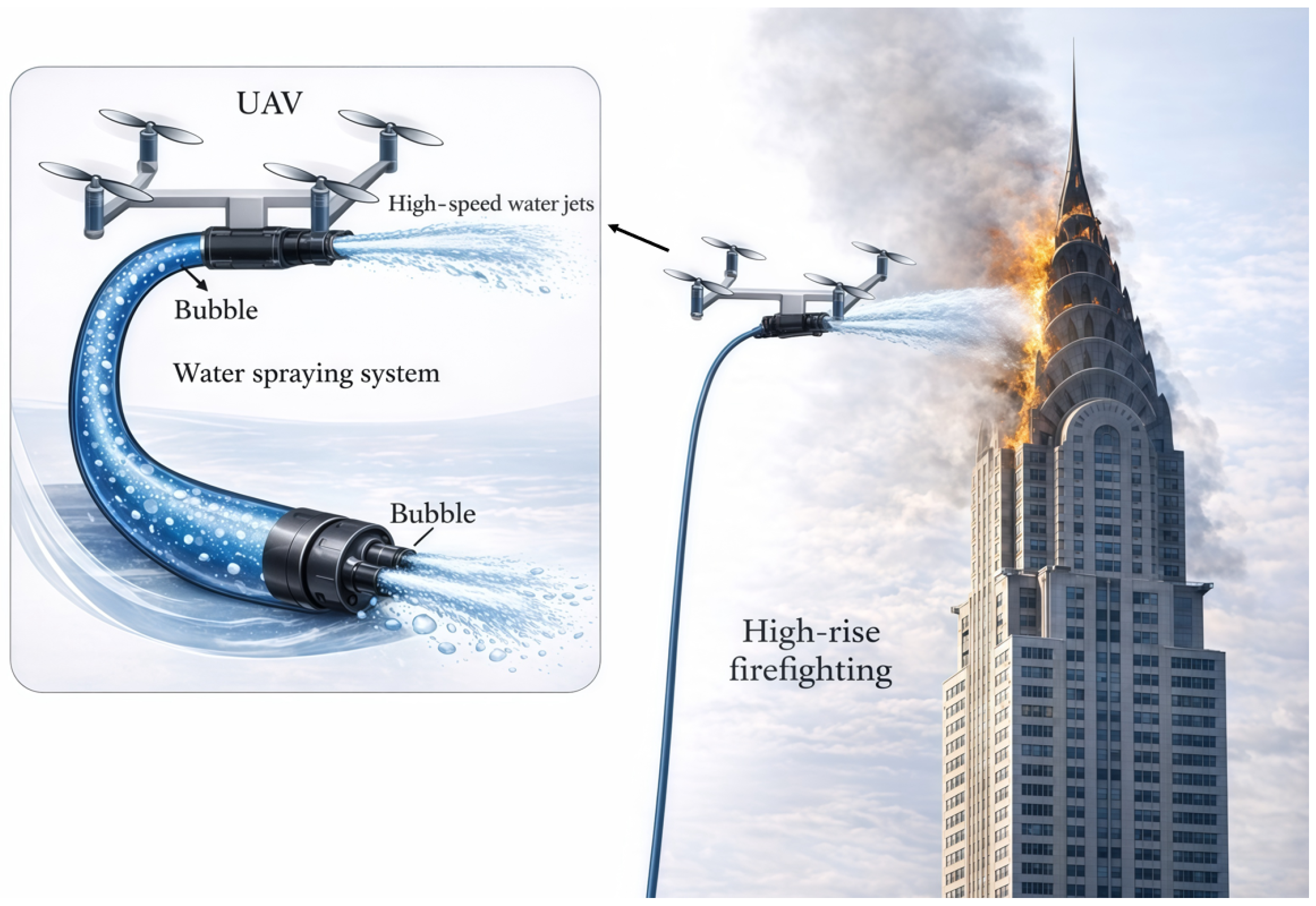
Unmanned aerial vehicles (UAVs) have emerged as promising tools for high-rise firefighting because they offer improved operational safety and deployment flexibility compared with conventional ground-based systems [1]. With the rapid growth of urban high-rise buildings, fire suppression in such environments has become increasingly challenging [2], since traditional firefighting approaches are often limited by insufficient reach, restricted accessibility, and slow deployment. UAV-mounted water-spraying systems provide a promising way to alleviate these limitations [3,4]. However, the high-speed water jets used for fire suppression generate strong reaction forces that can significantly disturb UAV flight dynamics and degrade stabilization performance, as illustrated in Figure 1 [5,6].
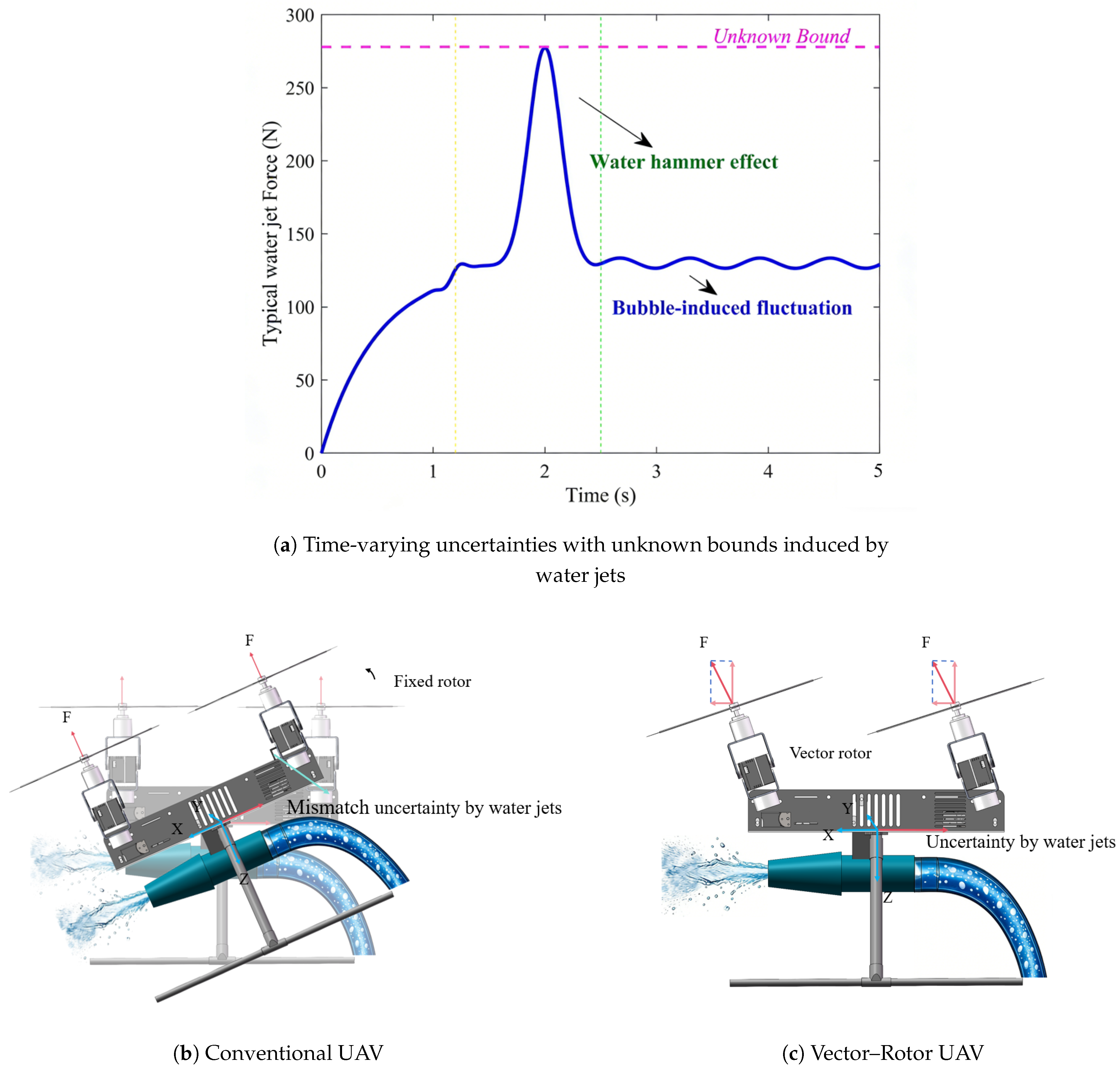
The control difficulty mainly arises from two aspects of water-jet dynamics. Firstly, conventional underactuated UAV architectures are inherently limited in compensating for water-jet-induced disturbances because their lateral motion is achieved through attitude adjustment [7], rather than through direct force generation along the disturbance direction [8,9]. Secondly, the fluid dynamics of water spraying (Figure 2a) introduce complex uncertainty patterns. These include transient water-hammer effects, which may produce pressure peaks two to three times higher than the steady-state level [10,11], and persistent bubble-induced flow fluctuations during continuous operation [12]. As a result, firefighting UAVs are subject to uncertainties that are not only strongly time-varying but also difficult to bound a priori [13]. These characteristics lead to two coupled control challenges: a mismatch between the vehicle actuation mechanism and the dominant disturbance direction, and the presence of fast time-varying uncertainties with unknown bounds.
Conventional quadrotor UAVs (QUAVs) (Figure 2b) [14] often have difficulty maintaining stable flight and accurate position regulation under the mismatch uncertainties induced by high-speed water jets because of their fixed-rotor architecture. By contrast, the vector–rotor UAV (VRUAV) studied in this paper adopts a fully actuated configuration with independently tiltable rotors (Figure 2c) [15], which enables decoupled control of translational motion and spraying direction. This configuration offers two main advantages. Firstly, it can generate thrust in multiple directions without requiring large body-attitude changes, thereby helping preserve the water-jet orientation during firefighting operations. Secondly, it can substantially alleviate the actuation–disturbance mismatch associated with conventional underactuated UAVs by reducing the dependence of horizontal motion on attitude reconfiguration [16,17]. Although this fully actuated architecture offers clear advantages for firefighting tasks [18,19,20], it also introduces stronger nonlinear coupling and more complex system dynamics, which place higher demands on controller design.
Most existing UAV control strategies are developed on the basis of model linearization. Such methods have achieved good performance in many conventional UAV applications. For example, Sadiq et al. [21] proposed a feedback linearization-based controller with uncertainty observers, while Yuan et al. [22] developed a feedback linearization–model predictive control (MPC) hybrid approach. However, the applicability of linearization-based methods becomes limited for VRUAV firefighting systems. These methods are typically most effective when rotor directions are fixed relative to the body frame and the vehicle operates in small-attitude conditions. In firefighting missions, however, the vehicle is often required to generate substantial horizontal force while operating with rotor tilting and pronounced nonlinear coupling, which weakens the validity and effectiveness of linearized control models.
To address these limitations, constraint-following control (CFC) provides a useful alternative for nonlinear mechanical systems. Pioneered by Chen et al. [23] and further developed in a series of studies by Sun et al. [24,25,26,27,28,29], CFC avoids direct model linearization and incorporates nonlinear motion constraints into controller design. Its control law is established from fundamental mechanical principles, such as Gauss’s principle of least constraint and d’Alembert’s principle, which makes it well suited to systems with strong nonlinearities and coupled dynamics. These features are particularly appealing for the present VRUAV, whose fully actuated yet strongly nonlinear structure is difficult to handle using conventional local linearization-based approaches.
In addition to strong nonlinearity, a second major challenge in VRUAV firefighting lies in the presence of fast time-varying uncertainties with unknown bounds, originating from both water-jet effects and system parameter variations. Such uncertainties can significantly deteriorate control performance if not properly compensated [30]. Existing methods, such as the backstepping sliding-mode controller proposed by Yu et al. [31] and the hybrid predictive control method reported in [32], often rely on constant or known uncertainty bounds. These assumptions, however, are difficult to justify in aerial firefighting scenarios, where the disturbance intensity may vary rapidly and irregularly. Adaptive control methods with online uncertainty estimation, such as the framework introduced by Chen et al. [33], provide an effective way to relax this requirement and have shown potential in a variety of complex systems [34,35,36,37,38].
Motivated by the above observations, this paper develops an adaptive robust constraint-following control (ARCFC) strategy for VRUAV state regulation under high-intensity time-varying water-jet disturbances. The proposed method combines the nonlinear mechanics-based formulation of CFC with online adaptive bound estimation, so that the controller can operate directly on the nonlinear dynamics without resorting to model linearization and without requiring prior knowledge of exact disturbance bounds. In the present study, the role of CFC is not merely to rewrite the regulation task in a constraint form. Rather, by embedding the desired spraying-state regulation objective into servo-constraints on the generalized motion, it provides a unified mechanical framework for constructing the nominal realization term, the stabilizing feedback term, and the uncertainty-compensation term.
The main contributions of this work are summarized as follows.
First, a VRUAV control framework is established for high-rise firefighting scenarios involving high-speed water spraying, in which the influence of water-jet-induced reaction forces and parametric uncertainties on flight stability is explicitly incorporated into the system dynamics.
Second, an ARCFC law is developed for nonlinear VRUAV state regulation under fast time-varying uncertainties with unknown bounds. The proposed controller integrates nominal constraint realization, stabilizing feedback, and adaptive robust compensation within a unified CFC framework.
Third, Lyapunov-based analysis is performed to establish the uniform boundedness and uniform ultimate boundedness of the closed-loop error system, and simulation studies under water-hammer-induced transient disturbance and bubble-induced rapidly varying disturbance are conducted to verify the effectiveness of the proposed method.

2. Problem Formulation

2.1. Dynamic Model of the VRUAV

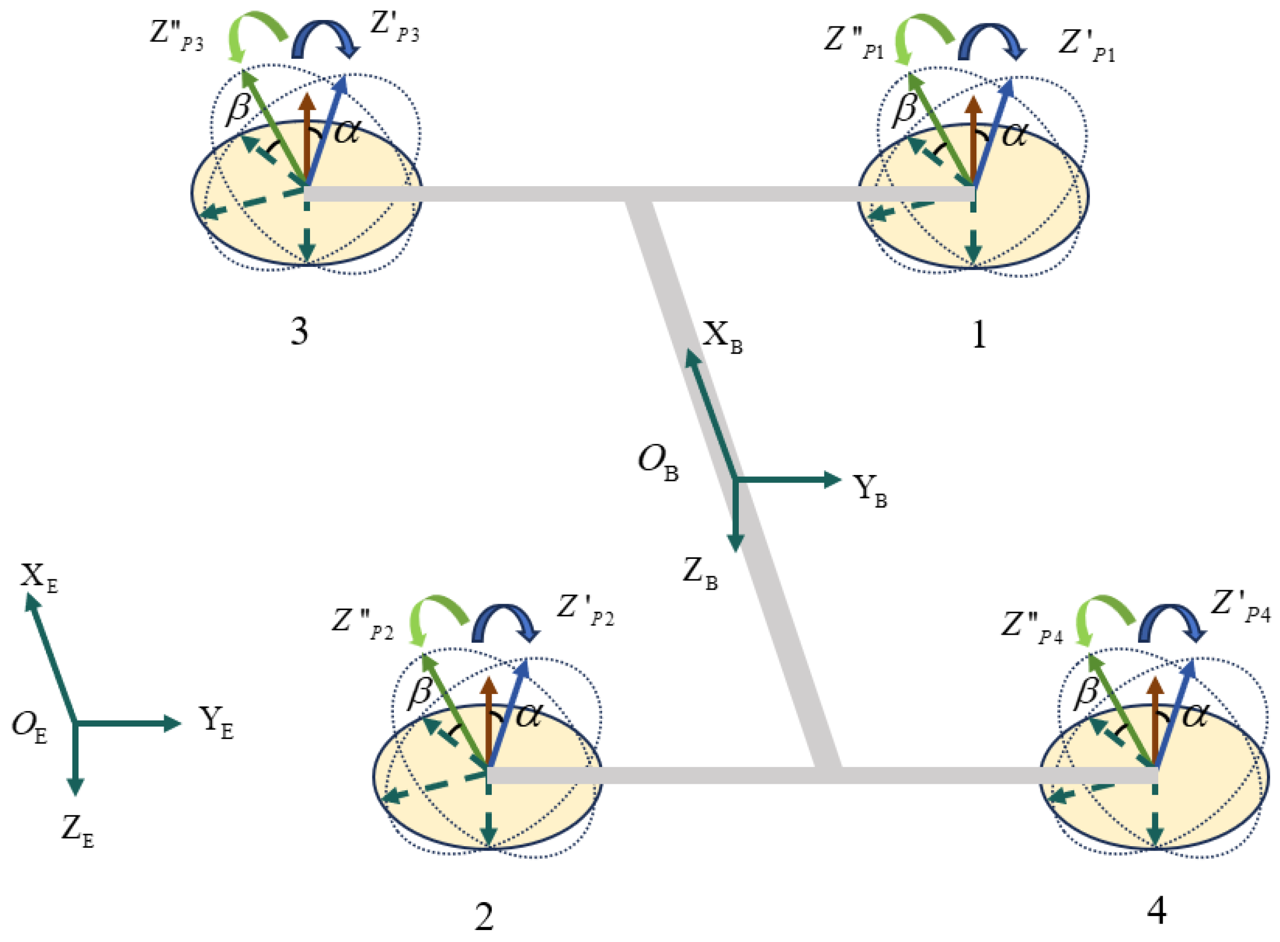
To resist the complex reaction forces generated by high-intensity water jets, the VRUAV considered in this paper is equipped with a thrust-direction modulation mechanism. The configuration of the VRUAV is illustrated in Figure 3. The motion of the VRUAV is described using two coordinate frames: the inertial frame E ( O E , X E , Y E , Z E ) and the body-fixed frame B ( O B , X B , Y B , Z B ) , whose origin is located at the center of gravity of the vehicle. The position and Euler-angle vectors of the VRUAV with respect to frame E are defined as ς = x y z T , ϵ = ϕ θ ψ T , respectively. In the firefighting task considered here, maintaining the VRUAV at a prescribed spraying position with a stable attitude is of primary importance.
Based on the above modeling, the uncertain dynamics of the VRUAV can be written as
M ( p ( t ) , ζ ( t ) , t ) p ¨ ( t ) + C ( p ˙ ( t ) , p ( t ) , ζ ( t ) , t ) p ˙ ( t ) + G ( p ( t ) , ζ ( t ) , t ) + K ( ζ ( t ) , t ) = u ( t )
where t R 0 denotes time, and ζ ( t ) R N is a possibly rapid and irregular time-varying uncertainty vector with unknown bounds, where N denotes the dimension of the uncertainty vector. The generalized state, velocity, and acceleration vectors are given by p , p ˙ , p ¨ R 6 , respectively, with p = x y z ϕ θ ψ T , p ˙ = x ˙ y ˙ z ˙ ϕ ˙ θ ˙ ψ ˙ T , and p ¨ = x ¨ y ¨ z ¨ ϕ ¨ θ ¨ ψ ¨ T . Moreover, u ( t ) R 6 denotes the generalized control input at the rigid-body level, and K ( ζ ( t ) , t ) R 6 denotes the generalized disturbance induced by the water-jet reaction. The matrices M ( · ) R 6 × 6 , C ( · ) R 6 × 6 , and G ( · ) R 6 represent the inertia matrix, Coriolis/centrifugal matrix, and gravity vector of the system, respectively. The detailed derivation of the dynamic model is provided in Appendix A.
In this paper, u ( t ) is generated by the upper-level nonlinear controller, while its realization in terms of individual rotor thrusts and tilting angles is handled by a lower-level control allocation module. Throughout the present analysis and simulations, this allocation is assumed to be feasible within the operating region of interest. Actuator saturation and allocation errors are not explicitly included in the current theoretical analysis and will be addressed in future work.

2.2. Control Objective

After reaching the designated spraying position, the VRUAV is required to maintain both its desired location and a stable attitude despite fluctuations in the reaction forces induced by the water jet. Specifically, the desired position components are x d , y d , and z d along the x-, y-, and z-axes, respectively, and the desired attitude components are ϕ d , θ d , and ψ d . Accordingly, the desired equilibrium state is defined as
p d = x d y d z d ϕ d θ d ψ d T .
Problem formulation: Design a control input u ( t ) for the uncertain nonlinear system (1) such that the VRUAV achieves bounded state regulation toward the desired equilibrium state (2) in the presence of possibly rapid and irregular time-varying uncertainties ζ ( t ) with unknown bounds.

3. Control Design

3.1. Constraint-Following Error

To simplify the subsequent derivations, the functional arguments of variables are omitted whenever no ambiguity is caused. We first consider the first-order servo-constraint that a general mechanical system is required to satisfy:
i = 1 n A l i ( p , t ) p ˙ i = c l ( p , t ) , l = 1 , , j ,
which can be written in matrix form as
A ( p , t ) p ˙ = c ( p , t ) ,
where A ( p , t ) = A l i ( p , t ) j × n , c ( p , t ) = c 1 c 2 c j T , and 1 j n . The functions A l i ( · ) and c l ( · ) are assumed to be continuously differentiable with respect to p and t. In general, the constraint in (4) may be non-integrable.
Differentiating (4) with respect to time yields
i = 1 n d A l i ( p , t ) d t p ˙ i + i = 1 n A l i ( p , t ) p ¨ i = d c l ( p , t ) d t ,
where
d A l i ( p , t ) d t = k = 1 n A l i ( p , t ) p k p ˙ k + A l i ( p , t ) t , d c l ( p , t ) d t = k = 1 n c l ( p , t ) p k p ˙ k + c l ( p , t ) t .
Therefore, the second-order form of the constraint can be expressed as
i = 1 n A l i ( p , t ) p ¨ i = i = 1 n d A l i ( p , t ) d t p ˙ i + d c l ( p , t ) d t = : b l ( p ˙ , p , t ) , l = 1 , , j ,
or, equivalently, in matrix form as
A ( p , t ) p ¨ = b ( p ˙ , p , t ) .
For the present spraying-state regulation task, the servo-constraint is constructed directly on the generalized states, and thus, A = [ I ] 6 × 6 . In this way, the desired equilibrium regulation objective is embedded into a unified servo-constraint form. The role of the CFC framework here is not merely to restate the control objective in a different notation; rather, it provides a mechanically interpretable basis for constructing the nominal realization term, the stabilizing feedback term, and the uncertainty-compensation term within a unified design.
By applying a suitable control input u, the controlled system can be made to satisfy the servo-constraint in (8) approximately. Based on (4), the corresponding constraint-following error is defined as
λ = A p ˙ c .
Accordingly, the regulation performance of the constrained motion can be characterized by λ = λ 1 λ 2 λ j T . If the control input u R 6 ensures that λ remains uniformly bounded for all admissible uncertainties, then the VRUAV can achieve bounded real-time regulation toward the desired equilibrium state.

3.2. Adaptive Robust Control Design

The system matrices and the water-jet-induced generalized disturbance are decomposed into nominal and uncertain parts as
M ( p , ζ , t ) = M ¯ ( p , t ) + Δ M ( p , ζ , t ) , C ( p , p ˙ , ζ , t ) = C ¯ ( p , p ˙ , t ) + Δ C ( p , p ˙ , ζ , t ) , G ( p , ζ , t ) = G ¯ ( p , t ) + Δ G ( p , ζ , t ) , K ( p , ζ , t ) = K ¯ ( p , t ) + Δ K ( p , ζ , t ) .
Here, M ¯ ( · ) , C ¯ ( · ) , G ¯ ( · ) , and K ¯ ( · ) denote the nominal parts, with M ¯ ( p , t ) > 0 , while Δ M ( · ) , Δ C ( · ) , Δ G ( · ) , and Δ K ( · ) represent the uncertain parts.
Assumption 1.
For the dynamic model of the VRUAV, the actual inertia matrix M ( p ) is assumed to be symmetric and strictly positive definite, i.e., M ( p ) > 0 , across the entire physically meaningful state space.
Define
D ( p , t ) : = M ¯ 1 ( p , t ) , Δ D ( p , ζ , t ) : = M 1 ( p , ζ , t ) M ¯ 1 ( p , t ) ,
and
E ( p , ζ , t ) : = I + M ¯ ( p , t ) M 1 ( p , ζ , t ) ,
so that
Δ D ( p , ζ , t ) = D ( p , t ) E ( p , ζ , t ) .
Accordingly, the nominal VRUAV model is written as
M ¯ ( p , t ) p ¨ ( t ) + C ¯ ( p , p ˙ , t ) p ˙ ( t ) + G ¯ ( p , t ) + K ¯ ( p , t ) = u ( t ) .
According to the nominal system (11) and the constraint (8), the nominal constraint force is given by
P 1 ( p , p ˙ , t ) : = M ¯ 1 2 ( p , t ) [ A ( p , t ) M ¯ 1 2 ( p , t ) ] + { b ( p ˙ , p , t ) + A ( p , t ) M ¯ 1 ( p , t ) [ C ¯ ( p , p ˙ , t ) p ˙ + G ¯ ( p , t ) + K ¯ ( p , t ) ] } .
The above term is constructed in the Lagrange form of d’Alembert’s principle so that the nominal system satisfies the imposed servo-constraint. When the model is exactly known, the control law based on (12) can enforce (8). However, in the presence of uncertainties, an additional robust adaptive compensation term is required.
For a given matrix h R 6 × 6 with h > 0 , define
U ( p , ζ , t ) : = h A ( p , t ) D ( p , t ) E ( p , ζ , t ) M ¯ ( p , t ) A T ( p , t ) A ( p , t ) A T ( p , t ) 1 h 1 .
Assume that there exists a constant ρ > 1 (possibly unknown) such that, for all ( p , t ) R 6 × R ,
1 2 min ζ Σ ϱ m U ( p , ζ , t ) + U T ( p , ζ , t ) ρ ,
where ϱ m ( · ) denotes the minimum eigenvalue. Since the uncertainty set Σ is unknown, the constant ρ is generally also unknown. When M = M ¯ , one has E = 0 , U = 0 , and thus, ρ = 0 . Hence, (14) characterizes an admissible deviation range between M and M ¯ .
Define further
P 2 ( p , p ˙ , t ) : = v M ¯ ( p , t ) A T ( p , t ) A ( p , t ) A T ( p , t ) 1 h 1 A ( p , t ) p ˙ c ( p , t ) ,
where v > 0 is a design constant.
We next introduce the following assumptions.
Assumption 2.
There exists an unknown constant vector η ( 0 , ) k and a known function
Π ( · ) : ( 0 , ) k × R 6 × R 6 × R R + ,
such that, for all  ( p , p ˙ , t ) R 6 × R 6 × R  and all  ζ Σ ,
( 1 + ρ ) 1 max ζ Σ h A Δ D C p ˙ G K + P 1 + P 2 h A D Δ C p ˙ + Δ G + Δ K Π ( η , p , p ˙ , t ) .
Assumption 3.
For all ( p , p ˙ , t ) R 6 × R 6 × R , the function Π ( · , p , p ˙ , t ) : ( 0 , ) k R + satisfies the following criteria:
(i) It is continuously differentiable;
(ii) It is concave with respect to η, i.e., for any η 1 , η 2 ( 0 , ) k ,
Π ( η 1 , p , p ˙ , t ) Π ( η 2 , p , p ˙ , t ) Π η ( η 2 , p , p ˙ , t ) ( η 1 η 2 ) ;
(iii) It is monotonically nondecreasing in each component of η.
Since ρ > 1 , it follows that 1 + ρ > 0 . The function Π ( · ) characterizes an upper bound associated with the uncertainties, while the unknown vector η is related to the uncertainty set Σ .
For some cases covered by Assumption 3, the function Π ( η , p , p ˙ , t ) may be linear in η , i.e., there exists a known function Π ^ ( · ) : R 6 × R 6 × R R + k such that
Π ( η , p , p ˙ , t ) = η T Π ^ ( p , p ˙ , t ) .
Based on the definition of the constraint-following error, the adaptive law is designed as
η ^ ˙ = ϱ 1 Π T η ( η ^ , p , p ˙ , t ) λ ( p , p ˙ , t ) ϱ 2 η ^ ,
where ϱ 1 > 0 and ϱ 2 > 0 are design constants.
The adaptive robust control law is then proposed as
u ( t ) = P 1 ( p , p ˙ , t ) + P 2 ( p , p ˙ , t ) + P 3 ( η ^ , p , p ˙ , t ) ,
with
P 3 ( η ^ , p , p ˙ , t ) : = M ¯ ( p , t ) A T ( p , t ) A ( p , t ) A T ( p , t ) 1 h 1 · γ ( η ^ , p , p ˙ , t ) μ ( η ^ , p , p ˙ , t ) Π ( η ^ , p , p ˙ , t ) .
where
μ ( η ^ , p , p ˙ , t ) = A ( p , t ) p ˙ c ( p , t ) Π ( η ^ , p , p ˙ , t ) ,
and
γ ( η ^ , p , p ˙ , t ) = 1 μ ( η ^ , p , p ˙ , t ) , μ ( η ^ , p , p ˙ , t ) > ξ , 1 ξ , μ ( η ^ , p , p ˙ , t ) ξ ,
with ξ > 0 being a small positive constant.
Remark 1.
It is worth noting that the design parameter ξ determines the trade-off between tracking accuracy and control effort in the proposed scheme. A smaller ξ permits a larger adaptation gain γ, resulting in increased control effort P 3 but a tighter ultimate error bound R, thereby improving tracking accuracy. Conversely, a larger ξ reduces the control effort while enlarging the tracking error bound. Therefore, ξ > 0 serves as a key tuning parameter for balancing control performance and control expenditure in practical applications.
In the above controller, P 3 serves as the adaptive robust compensation term. Since the unknown parameter vector η is unavailable, it is replaced by its estimate η ^ . In the adaptive law (19), the first term updates the parameter estimate according to the magnitude of the constraint-following error, whereas the second term is a leakage term that prevents parameter drift and improves robustness.
Remark 2.
Because the controlled system is subject to uncertain disturbances, the proposed controller is designed to guarantee the uniform boundedness and uniform ultimate boundedness of the closed-loop error signals rather than exact asymptotic convergence. The control law consists of three coordinated components: P 1 is the nominal constraint force used to realize the desired constrained dynamics; P 2 is a stabilizing feedback term for reducing the constraint-following error; and P 3 is an adaptive robust compensation term for handling uncertainties.
Compared with existing nonlinear control studies on disturbance-affected VRUAVs, the proposed method has the following distinguishing features. First, a VRUAV model subject to strong water-jet-induced disturbances is considered, in which the time-varying reaction effects of water spraying are explicitly taken into account. Second, by introducing the constraint-following error, the spraying-state regulation problem is reformulated as an approximate constraint-following problem, which makes it possible to design the controller directly on the nonlinear dynamics without resorting to model linearization. Third, on this basis, an adaptive robust controller is developed to handle uncertainties with unknown bounds online while maintaining moderate control effort.
Theorem 1.
Let
ϖ : = λ T ( η ^ η ) T T R m + k .
Under Assumptions 1–2, the closed-loop VRUAV system (1) with the controller (20) renders ϖ uniformly bounded and uniformly ultimately bounded.
Proof. 
Let
V ( λ , η ^ η ) = λ T h λ + ϱ 1 1 ( 1 + ρ ) ( η ^ η ) T ( η ^ η )
be a legitimate Lyapunov function candidate to prove the stability of the controller. Considering the uncertainties ζ ( · ) and the associated trajectories p ( · ) , p ˙ ( · ) and η ^ ( · ) , the derivative of V is obtained as
V ˙ ( λ , η ^ η ) = 2 λ T h λ ˙ + 2 ϱ 1 1 ( 1 + ρ ) ( η ^ η ) T η ^ ˙ .
Let the analysis proceed by examining every term in the equation on its own. The first step is to consider
2 λ T h λ ˙ = 2 λ T h ( A p ¨ b ) = 2 λ T h A M 1 ( C p ˙ G K ) + M 1 P 1 + P 2 + P 3 2 λ T h b ,
A M 1 ( C p ˙ G K ) + M 1 P 1 + P 2 + P 3 b = : V 1 .
Here, λ ˙ = A p ¨ b ; then, we have
V 1 = A [ ( D + Δ D ) ( C ¯ p ˙ G ¯ K ¯ Δ C p ˙ Δ G Δ K ) + ( D + Δ D ) P 1 + P 2 + P 3 b = A Δ D C p ˙ G K + P 1 + P 2 + D ( Δ C p ˙ Δ G Δ K ) + D ( C ¯ p ˙ G ¯ K ¯ ) + D P 1 + D P 2 + ( D + Δ D ) P 3 b .
V 2 : = Δ D C p ˙ G K + P 1 + P 2 + D ( Δ C p ˙ Δ G Δ K ) ,
V 3 : = D ( C ¯ p ˙ G ¯ K ¯ ) + D P 1 ,
V 4 : = D P 2 ,
V 5 : = ( D + Δ D ) P 3 .
For the nominal case, where ζ 0 and hence Δ M = Δ C = Δ G = Δ K = 0 , one has
V 3 = 0 .
According to Equation (16),
2 λ T h A V 2 2 λ h A V 2 2 ( 1 + ρ ) λ Π ( η , p , p ˙ , t ) .
By Equation (15), we have
2 λ T h A V 4 = 2 λ T h A D v M ¯ A T A A T 1 h 1 ( A p ˙ c ) = 2 v λ T ( A p ˙ c ) = 2 v λ 2 .
Because Δ D = D E , according to Equation (21), we have
2 λ T h A V 5 = 2 λ T h A D P 3 + 2 λ T h A D E P 3 .
Since P 3 = M ¯ A T A A T 1 h 1 γ μ Π ( η ^ , p , p ˙ , t ) , μ = λ ( η ^ , p , p ˙ , t ) , so
2 λ T h A D P 3 = 2 ( λ Π ( η ^ , p , p ˙ , t ) ) T γ μ = 2 γ μ 2 .
From Equation (13), together with Equation (14), and in accordance with the Rayleigh principle, we arrive at
2 λ T h A D E P 3 = 2 μ T h A D E P 3 2 γ μ T 1 2 ϱ m U + U T μ 2 γ ρ μ 2 .
Upon substituting Equation (37) into Equation (38), the following result is derived:
2 λ T h A V 5 2 γ ( 1 + ρ ) μ 2 .
According to Equation (23), if μ > ξ
2 γ ( 1 + ρ ) μ 2 = 2 ( 1 + ρ ) 1 μ μ 2 = 2 ( 1 + ρ ) μ ,
and if μ ξ
2 γ ( 1 + ρ ) μ 2 = 2 ( 1 + ρ ) 1 ξ μ 2 = 2 ( 1 + ρ ) μ 2 ξ .
Based on Equations (33)–(41), it can be concluded that if μ > ξ ,
2 λ T h λ ˙ 2 v λ 2 + 2 ( 1 + ρ ) { λ Π ( η ^ , p , p ˙ , t ) + λ Π ( η , p , p ˙ , t ) } ,
and if μ ξ ,
2 λ T h λ ˙ 2 v λ 2 2 γ ( 1 + ρ ) μ 2 ξ + 2 ( 1 + ρ ) λ Π ( η , p , p ˙ , t ) 2 v λ 2 + ( 1 + ρ ) ξ 2 + 2 ( 1 + ρ ) { λ Π ( η ^ , p , p ˙ , t ) + λ Π ( η , p , p ˙ , t ) } .
Next, by Assumption 2,
λ Π ( η ^ , p , p ˙ , t ) + λ Π ( η , p , p ˙ , t ) λ Π ( η ^ , p , p ˙ , t ) η ( η η ^ ) .
By replacing the second term on the right-hand side of Equation (25) into the adaptive law in Equation (19), we obtain
2 ϱ 1 1 ( 1 + ρ ) ( η ^ η ) T η ^ ˙ = 2 ϱ 1 1 ( 1 + ρ ) ( η ^ η ) T ϱ 1 Π T η ( η ^ , p , p ˙ , t ) λ ϱ 2 η ^ 2 ( 1 + ρ ) ( η ^ η ) T Π T η ( η ^ , p , p ˙ , t ) λ 2 ϱ 1 1 ϱ 2 ( 1 + ρ ) η ^ η 2 + 2 ϱ 1 1 ϱ 2 ( 1 + ρ ) η ^ η η .
By substituting Equations (44) and (45) into Equation (24) ( ϖ 2 = λ 2 + η ^ η 2 η ^ η     ϖ ) , we have
V ˙ 2 v λ 2 2 ϱ 1 1 ϱ 2 ( 1 + ρ ) η ^ η 2 + 2 ϱ 1 1 ϱ 2 ( 1 + ρ ) η ^ η η + ( 1 + ρ ) ξ 2 κ 1 ϖ 2 + κ 2 ϖ + κ 3 .
Here, κ 1 = min 2 v , 2 ϱ 1 1 ϱ 2 ( 1 + ρ ) , κ 2 = 2 ϱ 1 1 ϱ 2 ( 1 + ρ ) η , κ 3 = ( 1 + ρ ) ξ / 2 .
It then follows that the closed-loop system is uniformly bounded. Specifically,
(a) Uniform boundedness:
d ( r ) = χ 2 χ 1 R r R χ 2 χ 1 r r > R ,
R = 1 2 κ 1 κ 2 + κ 2 2 + 4 κ 2 κ 3 .
where χ 1 = min χ min ( h ) , ϱ 1 1 ( 1 + ρ ) , χ 2 = max χ max ( h ) , ϱ 1 1 ( 1 + ρ ) .
(b) Uniform ultimate boundedness:
d ¯ > d ̲ = χ 2 χ 1 R
L ( d ¯ , r ) = 0 r d ¯ χ 1 χ 2 χ 2 r 2 χ 1 2 / χ 2 d ¯ 2 κ 1 d ¯ 2 χ 1 / χ 2 κ 2 d ¯ χ 1 / χ 2 1 2 κ 3 r > d ¯ χ 1 χ 2 .
These expressions indicate that, by appropriately selecting the design parameters v, ϱ 1 , ϱ 2 , and ξ , the ultimate bound d ¯ can be made sufficiently small. □
Remark 3.
This section develops an adaptive robust controller for the VRUAV under water-spraying disturbances, based on the nonlinear dynamic model (1) and the constraint-following formulation introduced in Section 3.1.

4. Control Framework

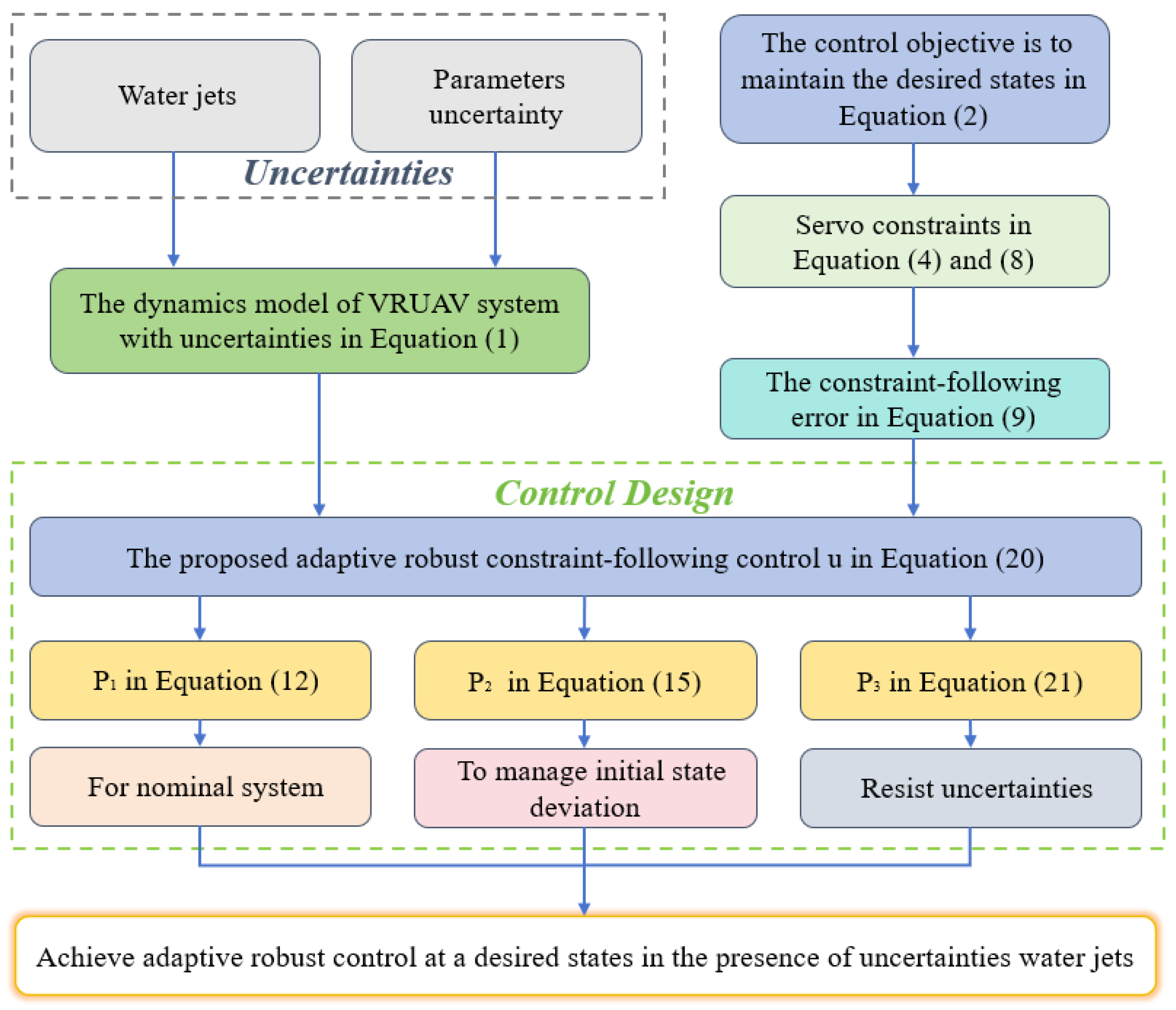
The overall control framework of the proposed ARCFC method for the VRUAV is illustrated in Figure 4. First, the nonlinear dynamics of the VRUAV are established with the explicit inclusion of water-jet-induced disturbances and parametric uncertainties. The desired spraying-state regulation objective is then converted into servo-constraints, from which the constraint-following error is derived. Based on this formulation, the generalized control input u is constructed as the sum of a nominal realization term P 1 , a stabilizing feedback term P 2 , and an adaptive robust compensation term P 3 . The resulting generalized command is subsequently delivered to the lower-level control allocation module to generate feasible rotor thrusts and tilting actions. Through this upper-level/lower-level architecture, the VRUAV achieves bounded state regulation under strong time-varying disturbances.

5. Simulation and Results

This section evaluates the ability of the proposed controller to suppress reaction forces induced by water spraying, which constitute the dominant source of uncertainty in the considered firefighting scenario. The ARCFC method is assessed through two representative disturbance cases and benchmarked against a sliding mode control (SMC) regulator. In addition, the structural effect of the VRUAV configuration is illustrated through comparison with the QUAV under the same disturbance conditions.

5.1. System Model and Parameters

To ensure fairness and reproducibility in the comparative simulations, the VRUAV and the QUAV are assigned identical mass, geometric dimensions, and inertia parameters. Specifically, both platforms have a mass of m ¯ = 50 kg ; moments of inertia I ¯ x x = 2.4 kg · m 2 , I ¯ y y = 2.4 kg · m 2 , and I ¯ z z = 3.0 kg · m 2 ; a wheelbase of d = 1.1 m ; and gravitational acceleration g = 9.8 N / kg . The detailed parameters are listed in Table 1.
The selected mass represents a heavy-duty UAV configuration for firefighting scenarios. For reference, industrial heavy-lift UAV platforms such as the DJI Agras T40 have a total weight of approximately 50 kg (including battery) and a maximum take-off weight of up to 90 kg. Although such platforms are primarily designed for spraying applications, they demonstrate that the selected mass falls within a realistic range for heavy-load multirotor UAV systems. The inertia parameters are selected consistently with the system mass.
Under high-intensity time-varying water-jet conditions, the uncertainties acting on the UAV mainly arise from the internal parametric uncertainties of the UAV itself and the external disturbances induced by the water jet. In this study, the mass and moments of inertia are treated as uncertain quantities in practical flight operations. Accordingly, these parameters are decomposed into nominal values and time-varying perturbations, namely
m = m ¯ + Δ m ( t ) , I = I ¯ + Δ I ( t ) ,
where Δ m ( t ) and Δ I ( t ) denote time-varying uncertainties in the mass and inertia, respectively. In the simulations, these uncertainty terms are specified as
Δ m ( t ) = 0.001 m ¯ sin ( t ) , Δ I ( t ) = 0.001 I ¯ sin ( t ) ,
so as to emulate small but time-varying parameter perturbations encountered in practical flight conditions.
It should be noted that in practical firefighting applications, the time-varying weight and the dynamic tension of the water hose are not explicitly modeled as coupled flexible dynamics; instead, they are reasonably incorporated into the lumped parametric uncertainties and external disturbances, which will be actively compensated for by the proposed ARCFC scheme.

5.2. Control Performance Under High-Intensity Fast Time-Varying Water-Jet Disturbances

To validate the effectiveness of the proposed controller under physically meaningful disturbance conditions, the water-jet-induced disturbances are modeled using two representative scenarios in this section. A benchmark SMC regulator is implemented for comparison with the proposed ARCFC method. SMC has been widely used in UAV control applications [39] and is therefore adopted here as a representative baseline. Based on the original system (1), the corresponding SMC dynamics are expressed as
M ¯ ( s ˙ ι q ˙ + p ¨ d ) + C ¯ p ˙ + G ¯ + K ¯ = u ,
where q = p p d , the sliding surface is defined as s = ι q + q ˙ , and the reaching law is given by
s ˙ = Λ sign ( s ) Θ s .

5.2.1. High-Intensity Transient Disturbance Caused by Water Hammer

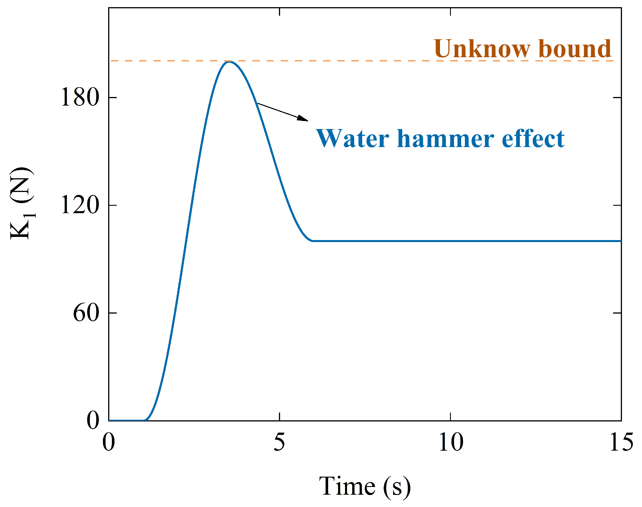
The water-hammer effect is equivalently modeled as an external transient disturbance acting on the UAV. This disturbance is suddenly introduced at a prescribed instant with bounded but unknown magnitude to characterize the impact caused by the rapid opening or closing of the nozzle. It then gradually decays toward the steady-state disturbance corresponding to normal water-spraying operation, as illustrated in Figure 5. Its mathematical expression is given by
K 1 ( t ) = K e n d + K s t a r t K e n d N ( t ) ,
where K s t a r t denotes the impulsive disturbance generated by the water-hammer effect, and K e n d denotes the steady disturbance associated with normal water spraying. The continuously differentiable transition function N ( t ) is defined as
N ( t ) = 0 , t < t 0 , sin 2 π ( t t 0 ) 2 T r + f , t 0 t t 0 + T r + f , 1 , t > t 0 + T r + f .
Here, t 0 denotes the starting time of the water jet, and T r + f denotes the duration of the transient transition process.
At the beginning of the simulation, the UAV is assumed to have already reached the firefighting target, and the initial state is set as
p 1 = 0 0 10 0 0 0 T .
The water jet is directed approximately along the positive x-axis of the body-fixed frame. In the experimental setup, the nozzle is mounted 20 cm below the center of mass of the VRUAV. At t = 1 s , the nozzle generates a water-hammer-induced transient disturbance. The ARCFC controller is first evaluated on both the QUAV and VRUAV platforms. For the QUAV system, the adaptive-law parameters are chosen as ϱ 11 = 0.1 and ϱ 12 = 0.1 . For the VRUAV system, the adaptive-law parameters are chosen as ϱ 21 = 0.1 and ϱ 22 = 0.1 . The corresponding results are shown below.
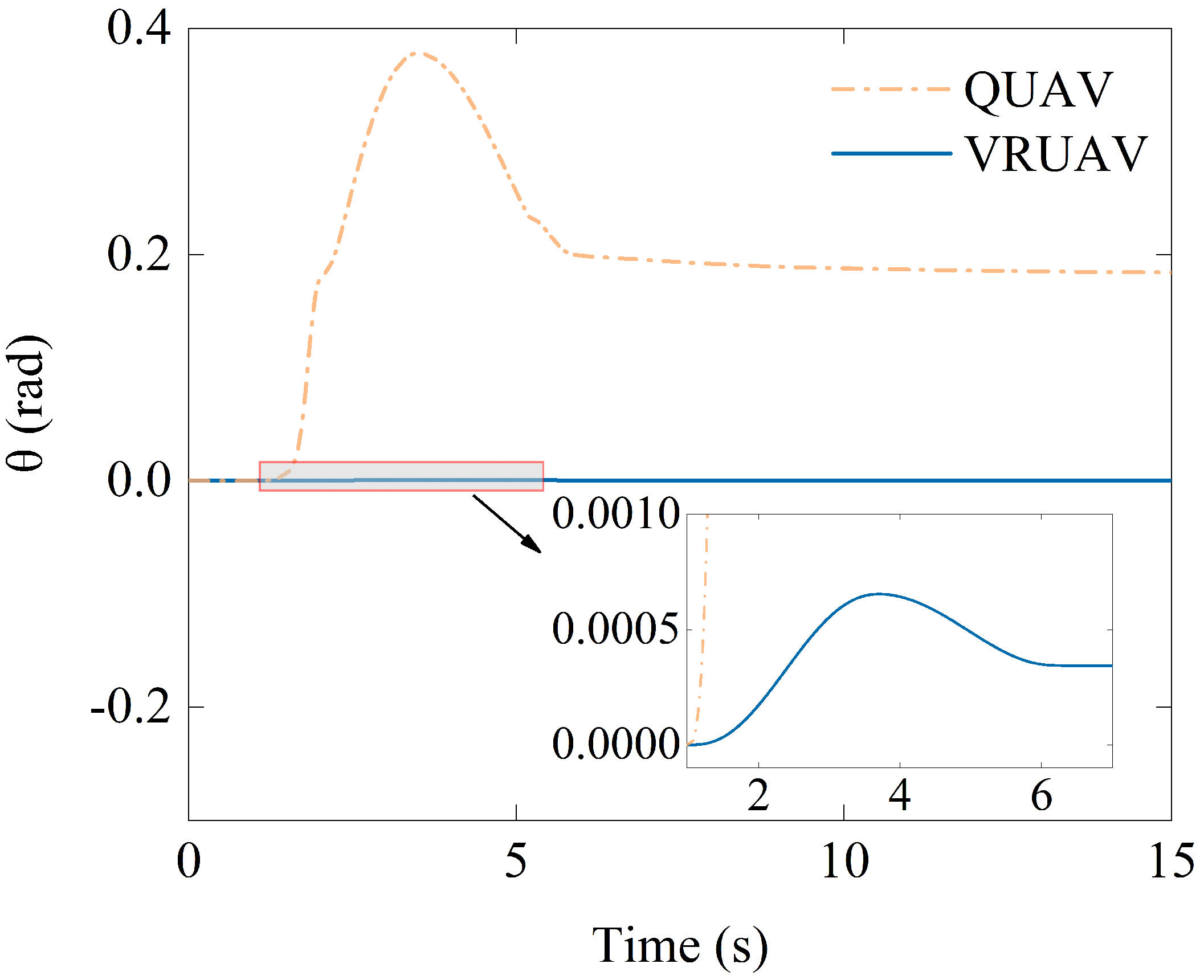
Figure 6 shows the pitch-angle responses of the QUAV and VRUAV under the transient water-jet disturbance. The QUAV converges to a nonzero pitch angle, whereas the VRUAV maintains its pitch angle in the vicinity of zero, with only negligible fluctuations throughout the disturbance process. Although both platforms can partially compensate for the disturbance, their compensation mechanisms are fundamentally different. The QUAV relies on body tilting to generate a balancing horizontal force, which inevitably changes the spraying direction in practical operation. In contrast, the VRUAV can resist the disturbance while maintaining an approximately horizontal attitude, which is more favorable for aerial firefighting tasks requiring stable jet orientation.
To further evaluate the proposed ARCFC method, it is compared with the SMC controller on the VRUAV platform. For the SMC law (51) under the water-hammer disturbance, the controller parameters are selected as
ι 1 = diag ( [ 10 , 10 , 5 , 5 , 5 , 5 ] ) , Λ 1 = diag ( [ 1 , 1 , 1.2 , 1.2 , 1.2 , 1.2 ] ) , Θ 1 = diag ( [ 1 , 1 , 1 , 1 , 1 , 1 ] ) .
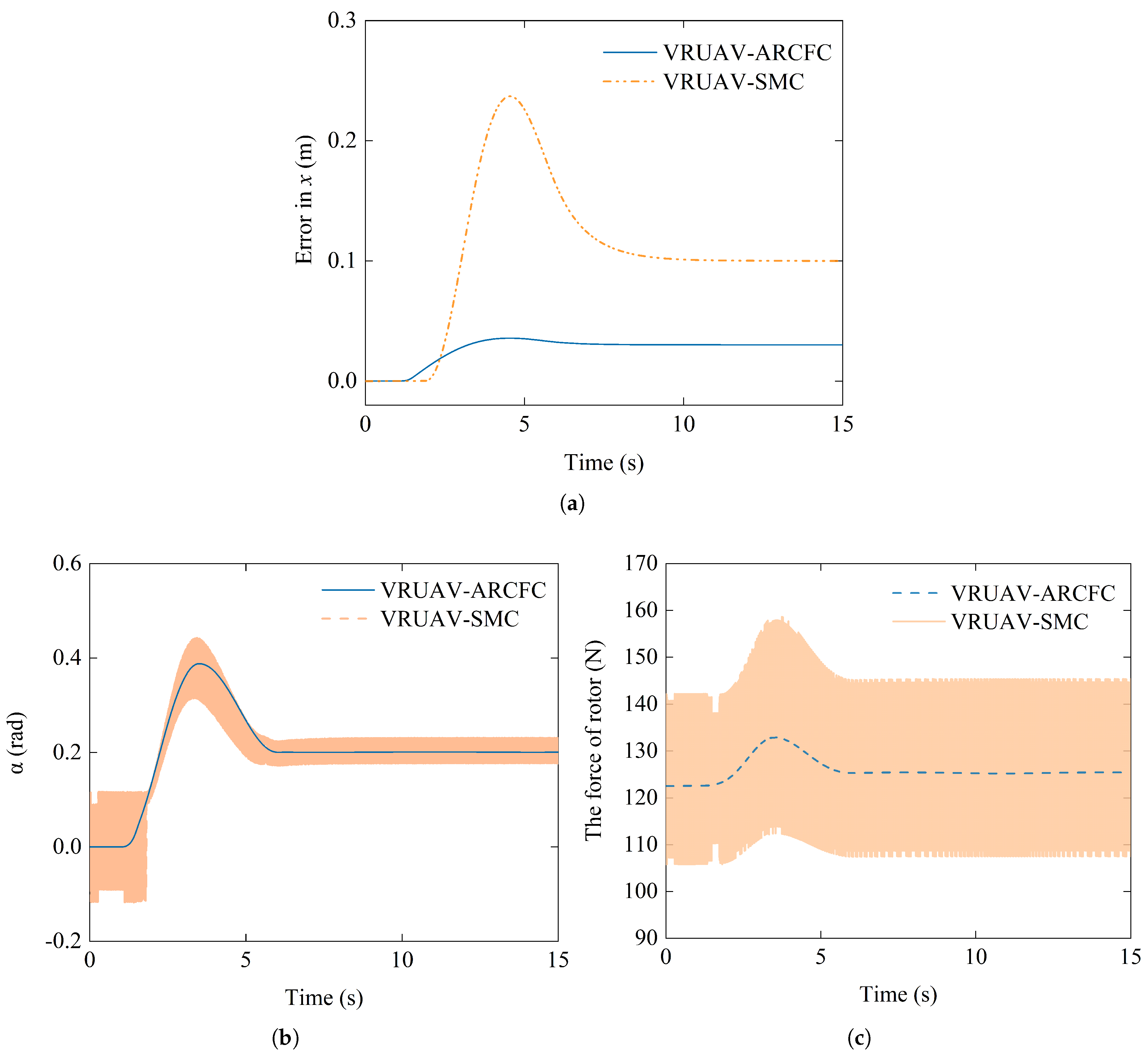
As shown in Figure 7a, under the transient water-hammer disturbance, the VRUAV controlled by SMC exhibits slower position recovery and a larger residual deviation along the x-axis. By contrast, the ARCFC controller confines the position error to a smaller range and drives the system back to the equilibrium state more rapidly. This indicates that the proposed controller achieves stronger disturbance rejection and better recovery performance under severe transient uncertainty.
Figure 7b compares the attitude responses of ARCFC and SMC. It can be observed that the SMC controller is more sensitive to the transient high-intensity disturbance and produces more pronounced oscillations in the tilt angle. In contrast, ARCFC suppresses the disturbance-induced attitude oscillation more effectively and yields a smoother attitude response.
Figure 7c presents the rotor control input generated by the two control strategies. The SMC controller exhibits more pronounced fluctuations throughout the simulation, indicating stronger sensitivity to the disturbance. By comparison, the ARCFC controller produces a smoother control input with a smaller overall magnitude. This suggests that the proposed controller not only preserves control performance but also reduces control effort.
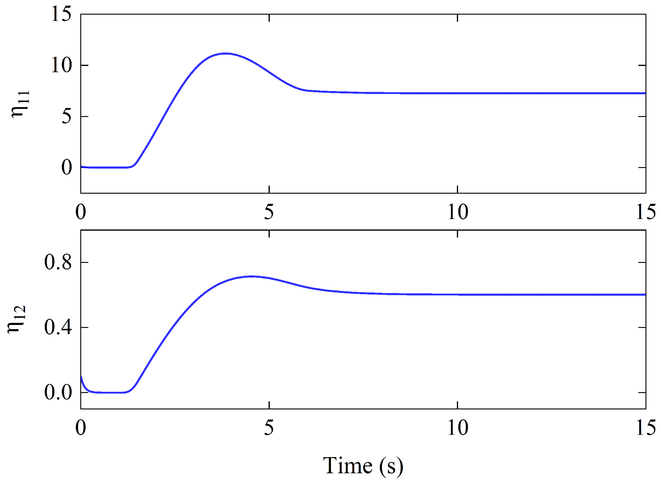
As shown in Figure 8, the adaptive parameters gradually decrease and converge to a bounded range. This behavior is due to the introduced leakage term, which prevents parameter drift once the state error becomes small and the disturbance is effectively compensated. The result is consistent with the boundedness analysis of the adaptive estimation process and closed-loop system.

5.2.2. Bubble-Induced Rapidly Varying Disturbances

The second scenario considers local flow instabilities caused by bubble generation and collapse, which make the reaction force acting on the UAV exhibit rapid and time-varying fluctuations. This effect is equivalently modeled as a time-varying periodic disturbance. Sinusoidal components are used to capture the dominant rapidly varying characteristics of the water-spraying disturbance, leading to the following model:
K 2 ( t ) = K s + A 1 cos ( 2 π f 1 t + l 1 ) + A 2 cos ( 2 π f 2 t + l 2 ) + W r ,
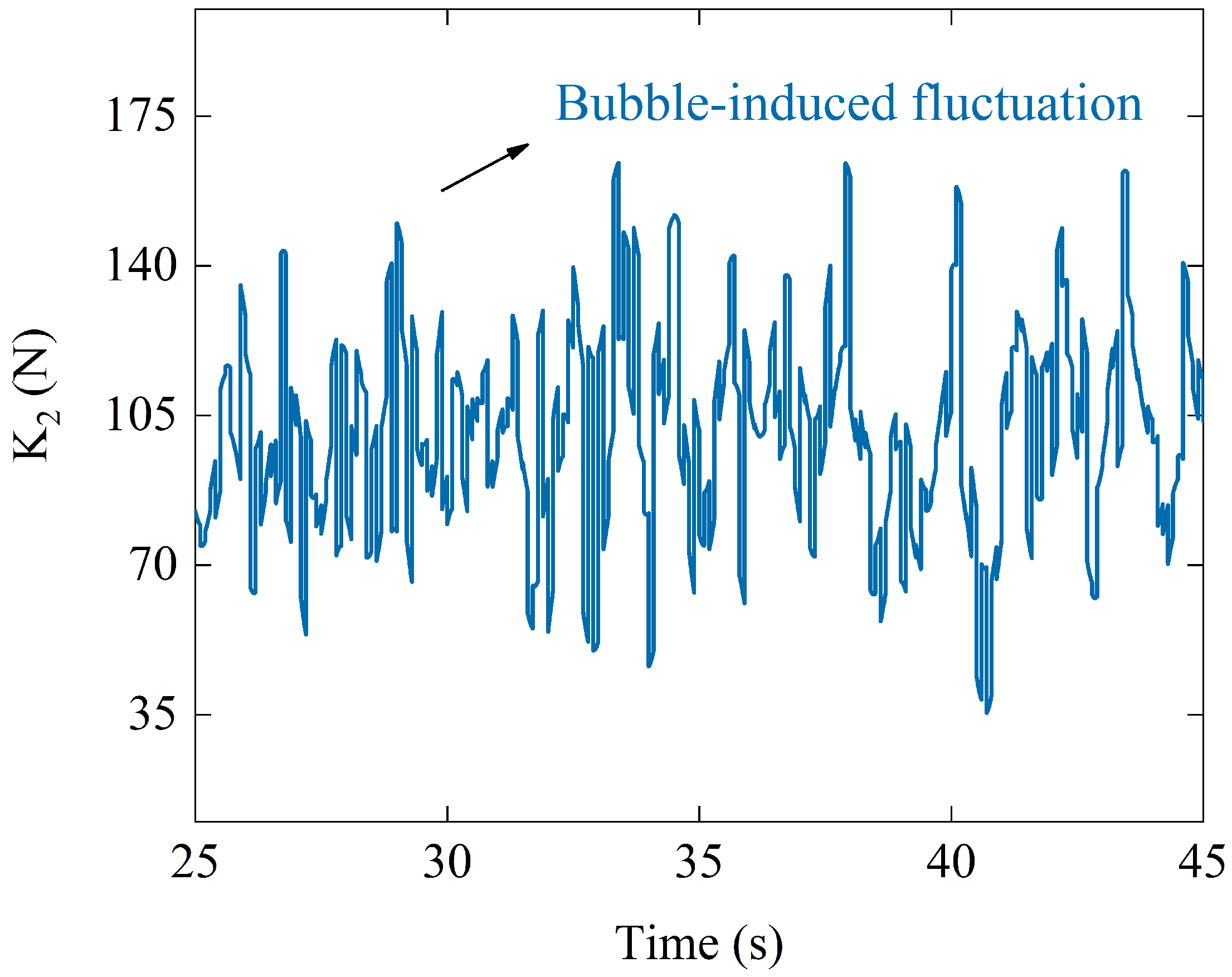
where K s denotes the steady disturbance associated with normal water spraying; A 1 and A 2 are the amplitudes of the disturbance components; f 1 and f 2 are their corresponding frequencies; and l 1 and l 2 denote the phase shifts. W r is defined as a zero-mean, unit-variance Gaussian stochastic process with a 100 Hz sampling frequency. It is postulated that all uncertainties and disturbances are bounded; however, the precise magnitudes of these bounds remain unknown a priori to the controller. The resulting disturbance profile is shown in Figure 9.
In this case, the UAV is assumed to have passed the initial transient stage of spraying and entered a stable spraying condition. The initial state is set as
p 2 = 0 0 10 0 0 0 T .
The water jet is generated by a nozzle mounted 20 cm below the center of mass of the VRUAV, and its direction remains aligned with the positive x-axis of the body-fixed frame. The bubble-induced rapidly varying disturbance is then applied to represent the oscillatory reaction force during sustained spraying. For the QUAV system, the adaptive-law parameters are selected as ϱ 31 = 0.5 and ϱ 32 = 0.5 . For the VRUAV system, the adaptive-law parameters are selected as ϱ 41 = 1 and ϱ 42 = 1 . The simulation results are shown below.
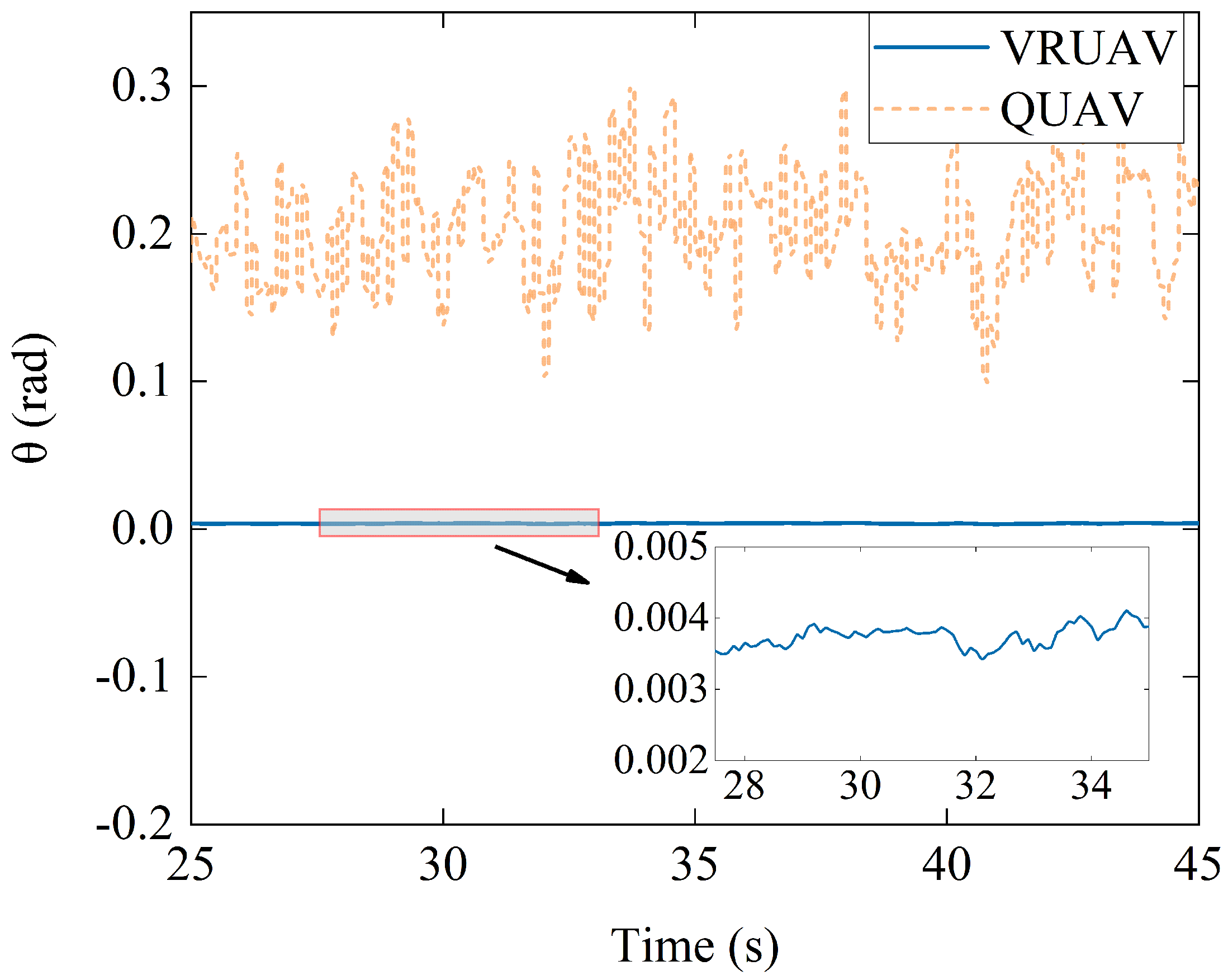
Figure 10 shows the pitch-angle responses of the QUAV and VRUAV under bubble-induced rapidly varying disturbance. The QUAV continuously adjusts its pitch angle to compensate for the oscillatory reaction force, which causes coupled fluctuations in the spraying direction. In contrast, the VRUAV experiences only minor pitch-angle deviations during the disturbance process, indicating its capability to suppress disturbance effects without requiring significant body-attitude adjustment.
To further assess disturbance-rejection performance, the proposed ARCFC method is again compared with SMC on the VRUAV platform. In this scenario, the SMC parameters in (51) are selected as
ι 2 = diag ( [ 15 , 15 , 3 , 3 , 3 , 3 ] ) , Λ 2 = diag ( [ 0.1 , 0.1 , 0.5 , 0.5 , 0.5 , 0.5 ] ) , Θ 2 = diag ( [ 1 , 1 , 5 , 5 , 5 , 5 ] ) .
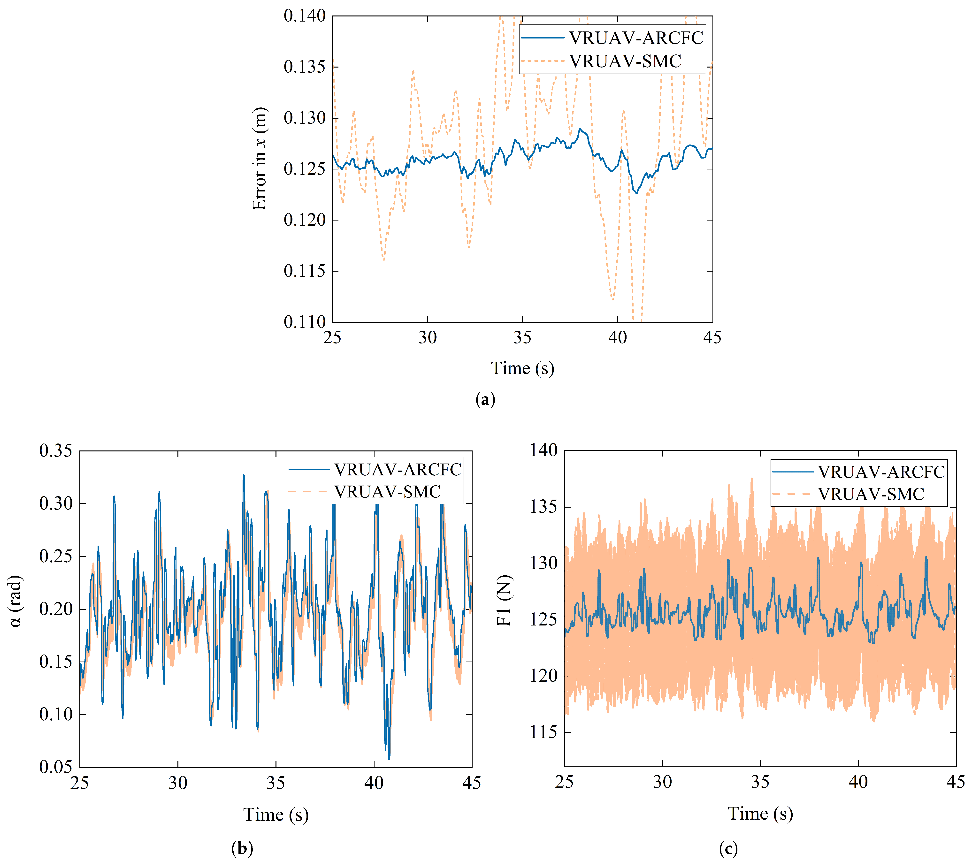
As shown in Figure 11a, under the rapidly varying disturbance, the SMC-controlled VRUAV exhibits larger deviation and weaker recovery performance along the x-axis. By comparison, the proposed ARCFC controller effectively confines the position error within a smaller range and restores the system state more quickly. These results indicate that ARCFC retains strong disturbance rejection and state-regulation capability even under fast time-varying uncertainty.
Figure 11b compares the tilt-angle responses of ARCFC and SMC under the rapidly varying disturbance. The SMC controller exhibits more pronounced oscillatory behavior, whereas ARCFC maintains a noticeably smoother attitude response. This result further shows that the proposed method is less sensitive to rapidly varying disturbance components.
Figure 11c shows the rotor control inputs produced by the two controllers. The SMC controller exhibits larger fluctuations and stronger sensitivity to high-frequency disturbance components. In contrast, the control input generated by ARCFC is smoother and has a smaller overall amplitude, indicating that the proposed controller can reduce control effort while maintaining satisfactory control performance.
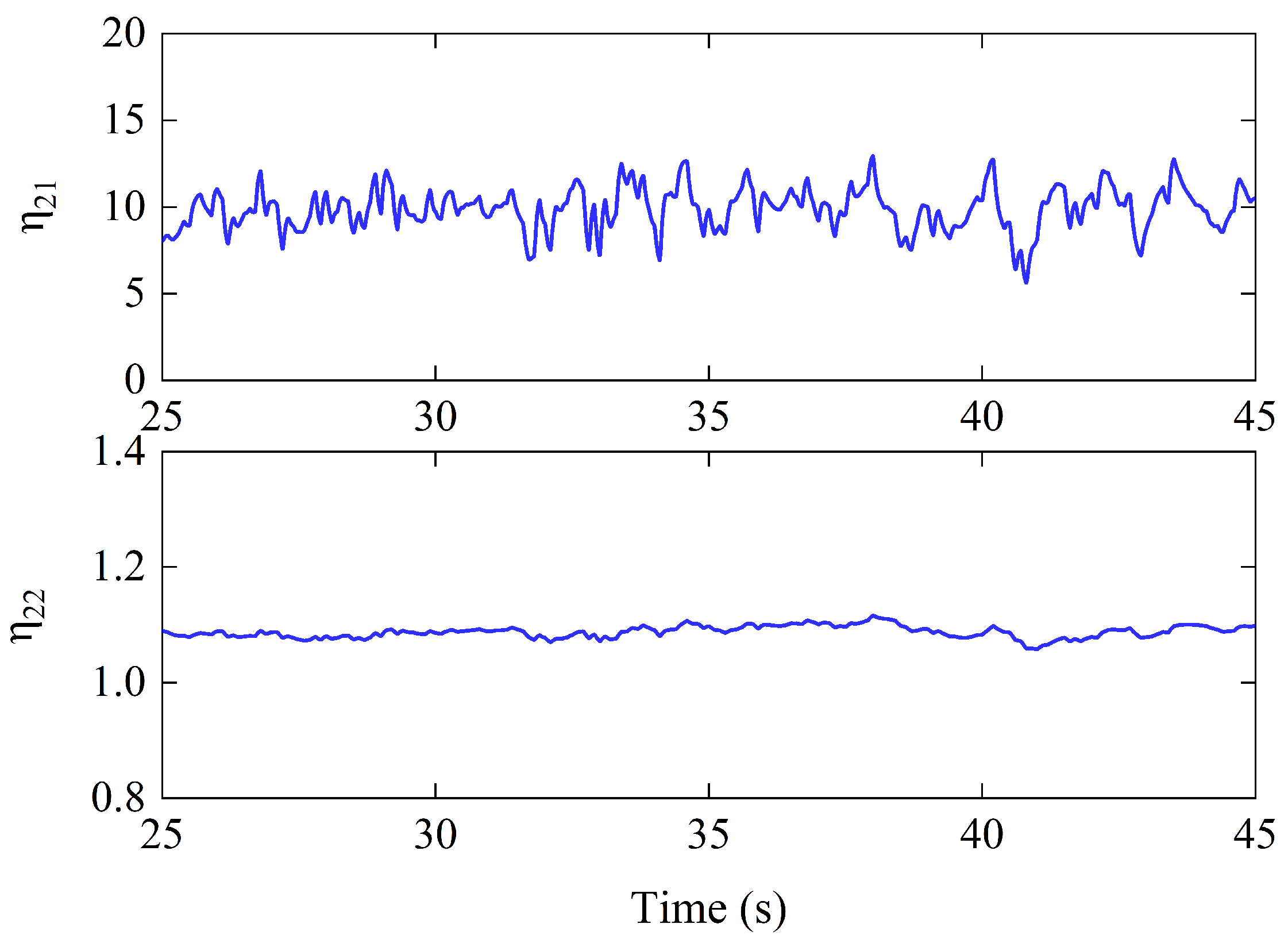
Finally, Figure 12 shows that the adaptive parameters remain bounded and converge into a stable range over time. Again, this behavior is attributed to the leakage term in the adaptive law, which suppresses parameter drift after the disturbance has been effectively compensated. This result is consistent with the theoretical boundedness properties established in the previous section.

6. Conclusions

This paper investigated the state-regulation problem of a VRUAV operating under high-intensity time-varying water-jet disturbances in high-rise firefighting scenarios. To address the strong nonlinearity of VRUAV dynamics and the presence of rapidly varying uncertainties with unknown bounds, an ARCFC strategy was proposed. By explicitly incorporating the generalized disturbance induced by water-jet reaction forces, the VRUAV’s dynamics under water-spraying conditions were established, and the regulation problem was reformulated as an approximate constraint-following problem through the introduction of the constraint-following error. Based on this framework, an adaptive robust controller was developed to compensate for uncertainties with unknown bounds, and Lyapunov-based analysis was carried out to establish uniform boundedness and uniform ultimate boundedness of the closed-loop error system. Simulation studies under two representative disturbance scenarios, namely water-hammer-induced transient disturbance and bubble-induced rapidly varying disturbance, showed that the proposed method enables the VRUAV to maintain the spraying direction more effectively than the QUAV configuration, while also achieving improved position regulation performance, smoother attitude responses, and lower control effort than the benchmark SMC regulator.
Future work will focus on hardware-in-the-loop and real-flight experimental validation, tighter integration between upper-level control and lower-level control allocation, and the extension of the proposed method to more realistic coupled aerodynamic–fluid disturbance environments.

Author Contributions

Conceptualization, Z.N. and Z.Z.; methodology, B.Z., J.D., and Z.N.; software, J.D. and Z.N.; validation, Z.N., X.Z., J.B., B.R., J.D., and Z.Z.; formal analysis, Z.N. and Z.Z.; investigation, Z.N. and Z.Z.; resources, Z.Z.; data curation, Z.N.; writing—original draft preparation, Z.N.; writing—review and editing, X.Z., J.B., B.R., B.Z., and Z.Z.; visualization, Z.N.; supervision, Z.Z., X.Z., J.B., B.R., and B.Z.; project administration, X.Z., J.B., B.R., and Z.Z.; funding acquisition, Z.Z. All authors have read and agreed to the published version of the manuscript.

Funding

This work was supported by the Key Research and Development Program in High-Tech Fields of Jiangxi Province under the Project ’Efficient Vector-Rotor UAV’, and the Hangzhou Innovation and Entrepreneurship Program for High-Level Overseas Returnees under the Project ’Strong-Wind-Resistant Omnidirectional Inspection Vector-Rotor UAV’.

Data Availability Statement

The related data and algorithms are presented within the manuscript. The datasets generated and/or analysed during the current study are available from the corresponding author on reasonable request.

Conflicts of Interest

The authors declare that they have no known competing financial interests or personal relationships that could have appeared to influence the work reported in this paper.

Abbreviations

The following abbreviations are used in this manuscript:
UAVUnmanned Aerial Vehicle
VRUAVVector–Rotor UAV
QUAVQuadrotor Unmanned Aerial Vehicle
CFCConstraint-Following Control
ARCFCAdaptive Robust Constraint-Following Control
SMCSliding Mode Control
MPCModel Predictive Control

Appendix A. Dynamic Modeling of the VRUAV
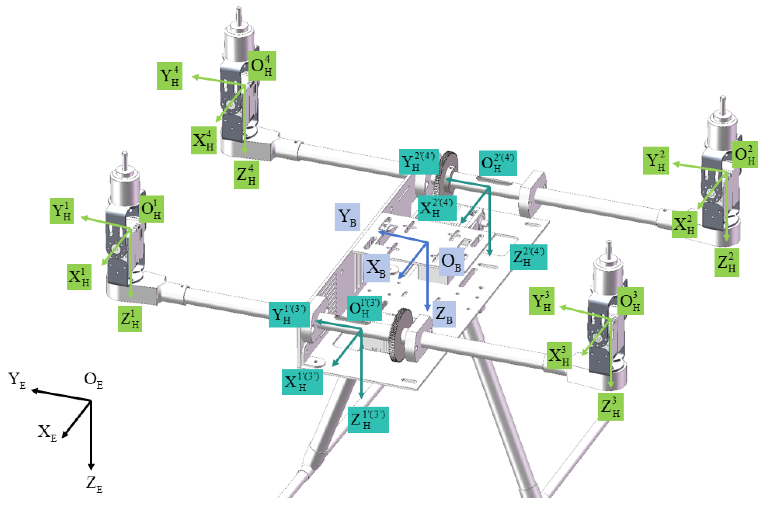
To support the compact uncertain model used in (1), this Appendix briefly outlines the rigid-body dynamics of the VRUAV with thrust-vectoring rotors. As shown in Figure A1, the vehicle motion is described by the inertial frame E ( O E , X E , Y E , Z E ) and the body-fixed frame B ( O B , X B , Y B , Z B ) . The translational position and Euler-angle vectors are denoted by
ς = x y z T , ϵ = ϕ θ ψ T .
The body angular velocity is denoted by
ω B = p B q B r B T ,
which is related to the Euler-angle rate through
ω B = 1 0 sin θ 0 cos ϕ sin ϕ cos θ 0 sin ϕ cos ϕ cos θ ϵ ˙ .
Each rotor can tilt with respect to the main body, so that its thrust direction is adjustable. For the ith rotor, let α i and β i denote the two tilting angles. The corresponding transformation from the rotor frame to the body-fixed frame can be written as
R H i B = R X H i ( β i ) R Y B ( α i ) 1 ,
where
R Y B ( α i ) = cos α i 0 sin α i 0 1 0 sin α i 0 cos α i , R X H i ( β i ) = 1 0 0 0 cos β i sin β i 0 sin β i cos β i .
Let Ω H i i and τ H i i denote the thrust vector and rotor torque generated in the ith rotor frame, respectively. Then the total force and total moment acting on the rigid body can be written as
F B = i = 1 4 R H i B Ω H i i , M B = i = 1 4 R H i B τ H i i + r i × R H i B Ω H i i ,
where r i is the position vector from the center of gravity to the ith rotor in the body-fixed frame.
Accordingly, the translational and rotational dynamics of the VRUAV are expressed as
m ς ¨ = R B E F B G ς + d f ( t ) ,
I ω ˙ B = M B ω B × ( I ω B ) + d τ ( t ) ,
where m and I denote the mass and inertia matrix of the VRUAV, respectively, G ς = [ 0 , 0 , m g ] T , and d f ( t ) and d τ ( t ) represent the force- and moment-level disturbances induced by water-jet reaction and other unmodeled effects.
By grouping the translational and rotational states into
p = x y z ϕ θ ψ T ,
and collecting the nominal actuation terms into the generalized input u ( t ) , the above dynamics can be arranged into the compact uncertain form
M ( p , ζ , t ) p ¨ + C ( p ˙ , p , ζ , t ) p ˙ + G ( p , ζ , t ) + K ( ζ , t ) = u ( t ) ,
which is the model adopted in (1). Here, K ( ζ , t ) collects the generalized disturbances caused by water-jet reaction as well as other time-varying uncertainties, while parametric variations are absorbed into the uncertain matrices and vectors of the compact model.
Figure A1. Coordinate definition and thrust-vectoring mechanism of the VRUAV.
Dynamics 06 00019 g0a1

References

  1. Perez-Saura, D.; Fernandez-Cortizas, M.; Perez-Segui, R.; Arias-Perez, P.; Campoy, P. Urban firefighting drones: Precise throwing from UAV. J. Intell. Robot. Syst. 2023, 108, 66. [Google Scholar] [CrossRef]
  2. Wang, K.; Yuan, Y.; Chen, M.; Lou, Z.; Zhu, Z.; Li, R. A study of fire drone extinguishing system in high-rise buildings. Fire 2022, 5, 75. [Google Scholar] [CrossRef]
  3. Viegas, C.; Chehreh, B.; Andrade, J.; Lourenço, J. Tethered UAV with combined multi-rotor and water jet propulsion for forest fire fighting. J. Intell. Robot. Syst. 2022, 104, 21. [Google Scholar] [CrossRef]
  4. Lee, S.M.; Ng, W.H.; Liu, J.; Wong, S.K.; Srigrarom, S.; Foong, S. Flow-Induced Force Modeling and Active Compensation for a Fluid-Tethered Multirotor Aerial Craft during Pressurised Jetting. Drones 2022, 6, 88. [Google Scholar] [CrossRef]
  5. Urazmetov, O.; Cadet, M.; Teutsch, R.; Antonyuk, S. Investigation of the flow phenomena in high-pressure water jet nozzles. Chem. Eng. Res. Des. 2021, 165, 320–332. [Google Scholar] [CrossRef]
  6. Handrick, D.; Eckenrode, M.; Lee, J. Review of Tethered Unmanned Aerial Vehicles: Building Versatile and Robust Tethered Multirotor UAV System. Dynamics 2025, 5, 17. [Google Scholar] [CrossRef]
  7. Emran, B.J.; Najjaran, H. A review of quadrotor: An underactuated mechanical system. Annu. Rev. Control 2018, 46, 165–180. [Google Scholar] [CrossRef]
  8. Çetinsoy, E.; Dikyar, S.; Hançer, C.; Oner, K.; Sirimoglu, E.; Unel, M.; Aksit, M. Design and construction of a novel quad tilt-wing UAV. Mechatronics 2012, 22, 723–745. [Google Scholar] [CrossRef]
  9. Franchi, A.; Carli, R.; Bicego, D.; Ryll, M. Full-pose tracking control for aerial robotic systems with laterally bounded input force. IEEE Trans. Robot. 2018, 34, 534–541. [Google Scholar] [CrossRef]
  10. Kumar, M.; Pu, J.H.; Hanmaiahgari, P.R.; Lambert, M.F. Insights into CFD Modelling of Water Hammer. Water 2023, 15, 3988. [Google Scholar] [CrossRef]
  11. Hsu, C.Y.; Liang, C.C.; Teng, T.L.; Nguyen, A.T. A numerical study on high-speed water jet impact. Ocean Eng. 2013, 72, 98–106. [Google Scholar] [CrossRef]
  12. Kiger, K.T.; Duncan, J.H. Air-entrainment mechanisms in plunging jets and breaking waves. Annu. Rev. Fluid Mech. 2012, 44, 563–596. [Google Scholar] [CrossRef]
  13. Eggers, J.; Villermaux, E. Physics of liquid jets. Rep. Prog. Phys. 2008, 71, 036601. [Google Scholar] [CrossRef]
  14. Walter, V.; Spurnỳ, V.; Petrlík, M.; Báča, T.; Žaitlík, D.; Demkiv, L.; Saska, M. Extinguishing real fires by fully autonomous multirotor UAVs in the MBZIRC 2020 competition. Field Robot. 2022, 2, 406–436. [Google Scholar] [CrossRef]
  15. Ahangar, A.R.; Ohadi, A.; Khosravi, M.A. A novel firefighter quadrotor UAV with tilting rotors: Modeling and control. Aerosp. Sci. Technol. 2024, 151, 109248. [Google Scholar] [CrossRef]
  16. Odelga, M.; Stegagno, P.; Bülthoff, H.H. A fully actuated quadrotor UAV with a propeller tilting mechanism: Modeling and control. In Proceedings of the IEEE International Conference on Advanced Intelligent Mechatronics (AIM), Banff, AB, Canada, 12–15 July 2016; pp. 306–311. [Google Scholar] [CrossRef]
  17. Ding, C.; Lu, L. A tilting-rotor unmanned aerial vehicle for enhanced aerial locomotion and manipulation capabilities: Design, control, and applications. IEEE/ASME Trans. Mechatron. 2020, 26, 2237–2248. [Google Scholar] [CrossRef]
  18. Kamel, M.; Verling, S.; Elkhatib, O.; Sprecher, C.; Wulkop, P.; Taylor, Z.; Siegwart, R.; Gilitschenski, I. The Voliro omniorientational hexacopter: An agile and maneuverable tiltable-rotor aerial vehicle. IEEE Robot. Autom. Mag. 2018, 25, 34–44. [Google Scholar] [CrossRef]
  19. Ryll, M.; Bülthoff, H.H.; Giordano, P.R. A novel overactuated quadrotor unmanned aerial vehicle: Modeling, control, and experimental validation. IEEE Trans. Control Syst. Technol. 2014, 23, 540–556. [Google Scholar] [CrossRef]
  20. Ryll, M.; Muscio, G.; Pierri, F.; Cataldi, E.; Antonelli, G.; Caccavale, F.; Franchi, A. 6D physical interaction with a fully actuated aerial robot. In Proceedings of the 2017 IEEE International Conference on Robotics and Automation (ICRA), Singapore, 29 May–3 June 2017; pp. 5190–5195. [Google Scholar] [CrossRef]
  21. Sadiq, M.; Hayat, R.; Zeb, K.; Al-Durra, A.; Ullah, Z. Robust Feedback Linearization Based Disturbance Observer Control of Quadrotor UAV. IEEE Access 2024, 12, 17966–17981. [Google Scholar] [CrossRef]
  22. Yuan, X.; Xu, J.; Li, S. Design and Simulation Verification of Model Predictive Attitude Control Based on Feedback Linearization for Quadrotor UAV. Appl. Sci. 2025, 15, 5218. [Google Scholar] [CrossRef]
  23. Chen, Y.H. Constraint-following servo control design for mechanical systems. J. Vib. Control 2009, 15, 369–389. [Google Scholar] [CrossRef]
  24. Sun, Q.; Yang, G.; Wang, X.; Chen, Y.H. Regulating constraint-following bound for fuzzy mechanical systems: Indirect robust control and fuzzy optimal design. IEEE Trans. Cybern. 2020, 52, 5868–5881. [Google Scholar] [CrossRef]
  25. Zhang, Z.; Zhang, B.; Yin, H. Constraint-based adaptive robust tracking control of uncertain articulating crane guaranteeing desired dynamic control performance. Nonlinear Dyn. 2023, 111, 11261–11274. [Google Scholar] [CrossRef]
  26. Yin, H.; Huang, J.; Chen, Y.H. Possibility-based robust control for fuzzy mechanical systems. IEEE Trans. Fuzzy Syst. 2020, 29, 3859–3872. [Google Scholar] [CrossRef]
  27. Sun, Q.; Yang, G.; Wang, X.; Chen, Y.H. Designing robust control for mechanical systems: Constraint following and multivariable optimization. IEEE Trans. Ind. Inform. 2019, 16, 5267–5275. [Google Scholar] [CrossRef]
  28. Fu, D.; Huang, J.; Yin, H. Controlling an uncertain mobile robot with prescribed performance. Nonlinear Dyn. 2021, 106, 2347–2362. [Google Scholar] [CrossRef]
  29. Yin, H.; Chen, Y.H.; Huang, J.; Lü, H. Tackling mismatched uncertainty in robust constraint-following control of underactuated systems. Inf. Sci. 2020, 520, 337–352. [Google Scholar] [CrossRef]
  30. Qin, W.; Shangguan, W.B.; Yin, H.; Chen, Y.H.; Huang, J. Constraint-following control design for active suspension systems. Mech. Syst. Signal Process. 2021, 154, 107578. [Google Scholar] [CrossRef]
  31. Yu, Z.; Zhang, J.; Wang, X. Thrust vectoring control of a novel tilt-rotor UAV based on backstepping sliding model method. Sensors 2023, 23, 574. [Google Scholar] [CrossRef] [PubMed]
  32. Sanna, D.; Madonna, D.P.; Pontani, M.; Gasbarri, P. Orbit rendezvous maneuvers in cislunar space via nonlinear hybrid predictive control. Dynamics 2024, 4, 609–642. [Google Scholar] [CrossRef]
  33. Chen, Y.H.; Zhang, X. Adaptive robust approximate constraint-following control for mechanical systems. J. Frankl. Inst. 2010, 347, 69–86. [Google Scholar] [CrossRef]
  34. Sun, H.; Tu, L.; Yang, L.; Zhu, Z.; Zhen, S.; Chen, Y.H. Adaptive robust control for nonlinear mechanical systems with inequality constraints and uncertainties. IEEE Trans. Syst. Man Cybern. Syst. 2022, 53, 1761–1772. [Google Scholar] [CrossRef]
  35. Zhao, H.; Liu, W.; Chen, X.; Sun, H. Adaptive robust constraint-following control for underactuated unmanned bicycle robot with uncertainties. ISA Trans. 2023, 143, 144–155. [Google Scholar] [CrossRef] [PubMed]
  36. Wang, X.; Wu, Z.; Sun, Q.; Ma, Y. Adaptive robust constraint-following control for electromechanically driven vector deflection system emphasis on time-varying uncertainty and input limit. Nonlinear Dyn. 2024, 112, 11167–11185. [Google Scholar] [CrossRef]
  37. Sun, H.; Chen, Y.H.; Zhao, H. Adaptive robust control methodology for active roll control system with uncertainty. Nonlinear Dyn. 2018, 92, 359–371. [Google Scholar] [CrossRef]
  38. Chen, X.; Zhao, H.; Sun, H.; Zhen, S.; Al Mamun, A. Optimal adaptive robust control based on cooperative game theory for a class of fuzzy underactuated mechanical systems. IEEE Trans. Cybern. 2020, 52, 3632–3644. [Google Scholar] [CrossRef] [PubMed]
  39. Shao, X.; Sun, G.; Yao, W.; Liu, J.; Wu, L. Adaptive sliding mode control for quadrotor UAVs with input saturation. IEEE/ASME Trans. Mechatron. 2021, 27, 1498–1509. [Google Scholar] [CrossRef]
Figure 1. High-speed water jets disturb UAV flight in high-rise firefighting.
Dynamics 06 00019 g001
Figure 2. Water-jet-induced disturbances and configuration comparison of UAV platforms. (a) Time-varying uncertainties with unknown bounds induced by water jets. (b) Conventional UAV. (c) Vector–rotor UAV.
Dynamics 06 00019 g002
Figure 3. Configuration and coordinate frames of the VRUAV.
Dynamics 06 00019 g003
Figure 4. Framework of the proposed ARCFC method for the VRUAV system.
Dynamics 06 00019 g004
Figure 5. Equivalent disturbance generated by the water-hammer effect.
Dynamics 06 00019 g005
Figure 6. Pitch-angle responses under water-hammer-induced disturbance.
Dynamics 06 00019 g006
Figure 7. System responses and performance comparison between the proposed ARCFC and SMC under water-hammer-induced disturbance. (a) x-axis position regulation errors. (b) Tilt-angle responses. (c) Rotor control input. The dense orange band in subfigures (b,c) is formed by the high-frequency oscillation (chattering) of the SMC curve.
Dynamics 06 00019 g007
Figure 8. Adaptive parameter evolution under water-hammer-induced disturbance.
Dynamics 06 00019 g008
Figure 9. Equivalent disturbance induced by bubble-related flow fluctuation.
Dynamics 06 00019 g009
Figure 10. Pitch-angle responses under bubble-induced rapidly varying disturbance.
Dynamics 06 00019 g010
Figure 11. System responses and performance comparison between the proposed ARCFC and SMC under bubble-induced rapidly varying disturbance. (a) x-axis position regulation errors. (b) Tilt-angle responses. (c) Rotor control input. Similar to Figure 7, the dense orange band in subfigure (c) is formed by the high-frequency oscillation (chattering) of the SMC curve.
Dynamics 06 00019 g011
Figure 12. Adaptive parameter evolution under bubble-induced rapidly varying disturbance.
Dynamics 06 00019 g012
Table 1. Simulation parameters.
ParameterDescriptionValue
m ¯ Mass of UAV50 kg
dWheelbase of UAV1.1 m
I ¯ x x Roll inertia of UAV2.4 kg·m2
I ¯ y y Pitch inertia of UAV2.4 kg·m2
I ¯ z z Yaw inertia of UAV3.0 kg·m2
gGravitational acceleration9.8 N/kg
Disclaimer/Publisher’s Note: The statements, opinions and data contained in all publications are solely those of the individual author(s) and contributor(s) and not of MDPI and/or the editor(s). MDPI and/or the editor(s) disclaim responsibility for any injury to people or property resulting from any ideas, methods, instructions or products referred to in the content.