A Coupled Reduced Theory for Depositional Onset on a Prescribed Two-Layer Bypass Background

Abstract

A recent two-layer theory for long-runout turbidity currents explains sustained bypass by allowing a dense lower layer to exchange mass with a more dilute upper layer while avoiding rapid over-thickening. Here, a morphodynamic extension is developed that couples suspended load and bed exchange while treating the two-layer hydrodynamics as a prescribed background. A suspended-sediment balance with bed exchange and Exner’s equation are written on that background, the depositional state variable $B=E_s/\left(rC\right)$ is introduced, and an exact nonlinear evolution equation for B is derived within the prescribed-background setting. In the weak-exchange limit this equation reduces to an algebraic onset criterion, thereby identifying the regime in which the simpler threshold is valid. Applied to an Amazon-like local-normal-flow reconstruction, the model shows that finite exchange shifts depositional onset upstream relative to the weak-exchange estimate. Background-fidelity checks, grid-refinement tests and closure/inlet sensitivities are reported to delimit the quantitative use of the reduced application. The framework is therefore best interpreted as a coupled reduced theory for suspended load and bed exchange on a prescribed two-layer bypass background rather than a fully hydro-morphodynamic closure.

1. Introduction

Long-runout turbidity currents transport suspended sediment through submarine canyons and channels over tens to hundreds of kilometres, and in some monitored systems over more than a thousand kilometres [1,2,3,4,5]. Their ability to remain mobile over such distances is now known to depend not only on bulk density contrast, but also on vertical structure. Direct observations in Monterey Canyon, for example, indicate fast dense basal layers overlain by more dilute clouds [6,7]. This layered structure is important because hydrodynamic survival of a current and depositional onset of its suspended load are not the same problem: a current may continue to bypass while the conditions for net deposition are gradually approached.

The first issue is therefore the physics of long-runout bypass. Classical sedimentological and experimental studies established the connection between turbidity currents, graded bedding and density-current motion [8,9,10,11,12]. Later theories of autosuspension and self-acceleration emphasized that erosion, suspended load and flow work can sustain long-distance transport [13,14,15]. Recent layer-averaged and reduced models continue this tradition by seeking the minimum structure needed to capture the persistence of sediment-laden gravity currents [16,17]. In particular, the two-layer formulation of Ma et al. [17] explains sustained bypass by allowing a dense lower layer to exchange mass with an overlying dilute layer while avoiding excessive lower-layer thickening.

The second issue is depositional onset. Fully resolved simulations, laboratory experiments and field studies show that suspension, settling and deposition are coupled processes whose signatures are filtered by flow structure, topography and preservation [18,19,20,21,22,23]. Yet many reduced descriptions of long-runout currents are built primarily to describe hydraulic persistence or bypass, not to identify where the bed first switches into net deposition. A useful reduced onset theory should therefore retain the layered long-runout background while adding a consistent suspended-sediment and bed-exchange balance.

The gap addressed here is precisely this reduced coupling problem. The paper develops a state-variable theory for depositional onset on a prescribed two-layer bypass background. The hydrodynamic fields imported from the parent model are the lower-layer velocity, lower-layer water flux and interfacial entrainment coefficient. On that background, a suspended-sediment balance with bed exchange is coupled to Exner’s equation. After the closure assumptions are specified, the depositional state variable is defined and shown to satisfy a closed nonlinear evolution equation. The weak-exchange limit recovers a transparent algebraic onset criterion, while the finite-exchange equation quantifies how suspended-load consistency shifts the onset location.

The contribution is thus deliberately limited in scope. The theory is coupled in suspended load and bed exchange, but it is not a full hydro-morphodynamic calculation in which the evolving bed feeds back onto the two-layer hydrodynamics. The Amazon-like calculation is used as an illustrative reduced-model benchmark: it shows how the theory diagnoses the competition among velocity decay, dilution, stratification-sensitive suspension capacity and finite exchange. It is not presented as a quantitative prediction for a particular natural system.

2. Model Setup: Prescribed Two-Layer Bypass Background

This section is part of the model formulation. It specifies which fields are imported from the parent two-layer theory and which variables are evolved by the reduced morphodynamic problem. The aim is not to reproduce the full parent model, but to define a prescribed long-runout bypass background on which suspended load and bed exchange can be treated consistently.

2.1. Background Fields Imported from the Parent Theory

The steady, one-dimensional, supercritical bypass branch of the two-layer model of Ma et al. [17] is adopted as a prescribed hydrodynamic background. The lower-layer and upper-layer velocities are denoted by $U_L$ and $U_U$, their thicknesses by ${\delta }_L$ and ${\delta }_U$, and the lower-layer depth-averaged concentration by C. The lower-layer water flux is

$$q_w=U_L{\delta }_L.$$

(1)

The interfacial entrainment coefficient is denoted by $e_{ws}\left(x\right)$ and inherits the stratification dependence of the parent theory through the interfacial Richardson number [17].

This reduction does not assume that the suspended sediment flux remains constant once bed exchange is admitted. Instead, the bypass branch is used only to prescribe the background functions

$$U_L\left(x\right),q_w\left(x\right),e_{ws}\left(x\right),$$

(2)

which are then coupled to suspended-sediment evolution and Exner’s equation in Section 3. This distinction is the key modelling choice adopted here.

2.2. Local-Normal-Flow Reconstruction

To obtain a tractable analytical background, a local-normal-flow reduction is adopted. The bed slope $S\left(x\right)$ is assumed to vary slowly enough that the lower-layer state can be approximated by a locally selected normal-flow branch,

$$U_L\left(x\right)\approx U_{Ln}\left(S\left(x\right)\right),q_w\left(x\right)\approx q_{wn}\left(S\left(x\right)\right),e_{ws}\left(x\right)\approx e_{ws,n}\left(S\left(x\right)\right).$$

(3)

The upper-layer velocity is written in the reduced form

$$U_U=\Gamma U_L,0<\Gamma <1,$$

(4)

with $\Gamma$ inherited from the parent branch. This is not a replacement for the full downstream integration of Ma et al. [17]; it is a slow-background approximation that isolates the onset problem on top of the long-runout hydrodynamics.

Three qualitative features of the parent solution are crucial. First, the lower-layer velocity relaxes rapidly toward the locally selected normal-flow value. Secondly, the lower-layer thickness evolves much more slowly than in depth-averaged single-layer theories. Thirdly, the bypass branch remains hydrodynamically viable over long downstream distances because settling-related detrainment inhibits runaway thickening [17]. These features are the background on which the morphodynamic problem is posed.

3. Coupled Reduced Morphodynamics on the Prescribed Background

3.1. Suspended-Sediment and Bed-Exchange Balances

At leading order, bedload is neglected, so the reduced Exner equation is written as

$$(1-\lambda ){\eta }_t=-{\partial }_x{q}_b+v_s(rC-E_s)\approx v_s(rC-E_s),$$

(5)

where $v_s$ is the settling velocity, $E_s$ is the dimensionless bed-entrainment coefficient into suspension, and r is the ratio of near-bed concentration to lower-layer depth-averaged concentration.

The steady suspended-sediment equation on the prescribed background is

$${\displaystyle \frac{\mathrm{d}}{\mathrm{d}x}}\left(q_{w}C\right)=v_s(E_s-rC).$$

(6)

Equations (5) and (6) are consistent: any gain or loss of suspended sediment in the lower layer is matched by an equal and opposite loss or gain of bed material.

3.2. Closure and State Variable

The reduced closure assumes

$$q_b\simeq 0,r=r_0,u_{*}^2=C_{fb}{U}_L^2,$$

(7)

These assumptions allow the suspended-load entrainment coefficient to be written in the dimensionless normalized form:

$${\displaystyle \frac{E_s\left(x\right)}{E_{s0}}}={\left({\displaystyle \frac{u_{*}\left(x\right)}{u_{*0}}}\right)}^p{\left({\displaystyle \frac{e_{ws}\left(x\right)}{e_{ws,0}}}\right)}^{\beta },p>0,\beta \ge 0.$$

(8)

where $E_{s0}=B_{\mathrm{in}}{r}_0{C}_0$ fixes the upstream calibration, and the reference case uses $B_{\mathrm{in}}=1$. This form makes the dimensional status of the closure explicit: K is not an additional dimensional constant in the reduced problem, but is absorbed into the upstream reference level $E_{s0}$. The exponent p measures the shear sensitivity of entrainment, while $\beta$ quantifies the suppression of entrainment as interfacial mixing weakens relative to the upstream value $e_{ws,0}$. The closure remains reduced and intentionally effective: it is not proposed as a universal transport law, but as a controlled sensitivity model that lets bed exchange feel both bed shear and the interfacial suppression already present in the parent two-layer hydrodynamics.

The closure (8) should be read as an intentionally effective structural closure rather than as a universal entrainment law. The factor $u_{*}^p$ preserves the classical idea that bed entrainment strengthens with bed shear, whereas the factor ${(e_{ws}/e_{ws,0})}^{\beta }$ uses the parent-model interfacial entrainment coefficient as an effective proxy for the turbulence capacity of the dense lower layer. It is not interpreted as a literal near-bed variable in the reduced model. In the parent two-layer background, $e_{ws}$ decreases as the interfacial Richardson number increases [17]. In the reduced morphodynamic setting this is taken to imply that stronger interfacial suppression also weakens the ability of the lower layer to maintain sediment in suspension near the bed. The exponent $\beta$ therefore packages unresolved links among shear production, near-bed concentration structure and turbulence suppression. In that sense the closure blends three familiar viewpoints rather than replacing them: Shields-type dependence enters through $u_{*}$, Rouse-type suspension capacity through the competition between entrainment and settling encoded in $B=E_s/\left(rC\right)$, and García–Parker-style thinking through the use of an effective entrainment coefficient rather than a first-principles turbulence closure [24,25,26]. The closure is thus best interpreted as a reduced sensitivity model with physically motivated ingredients, not as a final constitutive law. Experimental and numerical studies of sediment-laden stratified layers further support this cautious interpretation: dense suspended layers can entrain, settle and suppress turbulence in ways that depend on both local shear and stratification [27,28,29]. Those results do not determine the exponent $\beta$ directly, but they justify treating stratification-sensitive turbulence capacity as an explicit control in a reduced onset model.

The remaining closure choices are equally reduced. The near-bed concentration ratio is held fixed, $r=r_0$, to isolate the effect of velocity decay, dilution, interfacial suppression and finite exchange on the onset threshold. Allowing r to vary downstream would add another closure for the vertical concentration structure and would shift the threshold quantitatively, but it would not change the form of the state-variable balance. Bedload is neglected for the same reason: the present model is designed to examine suspended-load exchange from the dense lower layer to the bed. Coarser-grained or near-bed traction-dominated currents would require a bedload term in Exner’s equation and are outside the scope of this first reduced theory.

Define the depositional state variable:

$$B\left(x\right)={\displaystyle \frac{E_s\left(x\right)}{r_{0}C\left(x\right)}}.$$

(9)

Then, $B>1$ corresponds to net erosion, $B=1$ to local bypass, and $B<1$ to net deposition. The upstream boundary is normalized by taking

$$B\left(0\right)=1,$$

(10)

i.e., locally bypassing conditions at the inlet. The normalization $B\left(0\right)=1$ is convenient because it fixes the inlet state to local bypass and absorbs the coefficient K into the upstream reference level. More generally, one could prescribe an inlet value $B\left(0\right)=B_{\mathrm{in}}\ne 1$, in which case the exact transformed problem introduced below and the weak-exchange expansion remain unchanged apart from the initial condition $Y\left(0\right)=1/B_{\mathrm{in}}$. The onset problem would then concern the first downstream crossing of $B=1$ from the appropriate side rather than a return to unity from a bypassing inlet.

For the Amazon-like backgrounds considered here, the upstream drift is initially positive, so the solution first enters a non-depositional branch ($B>1$) before returning to unity. The onset definition therefore corresponds to a genuine first downstream return.

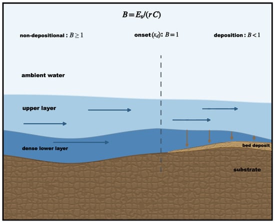
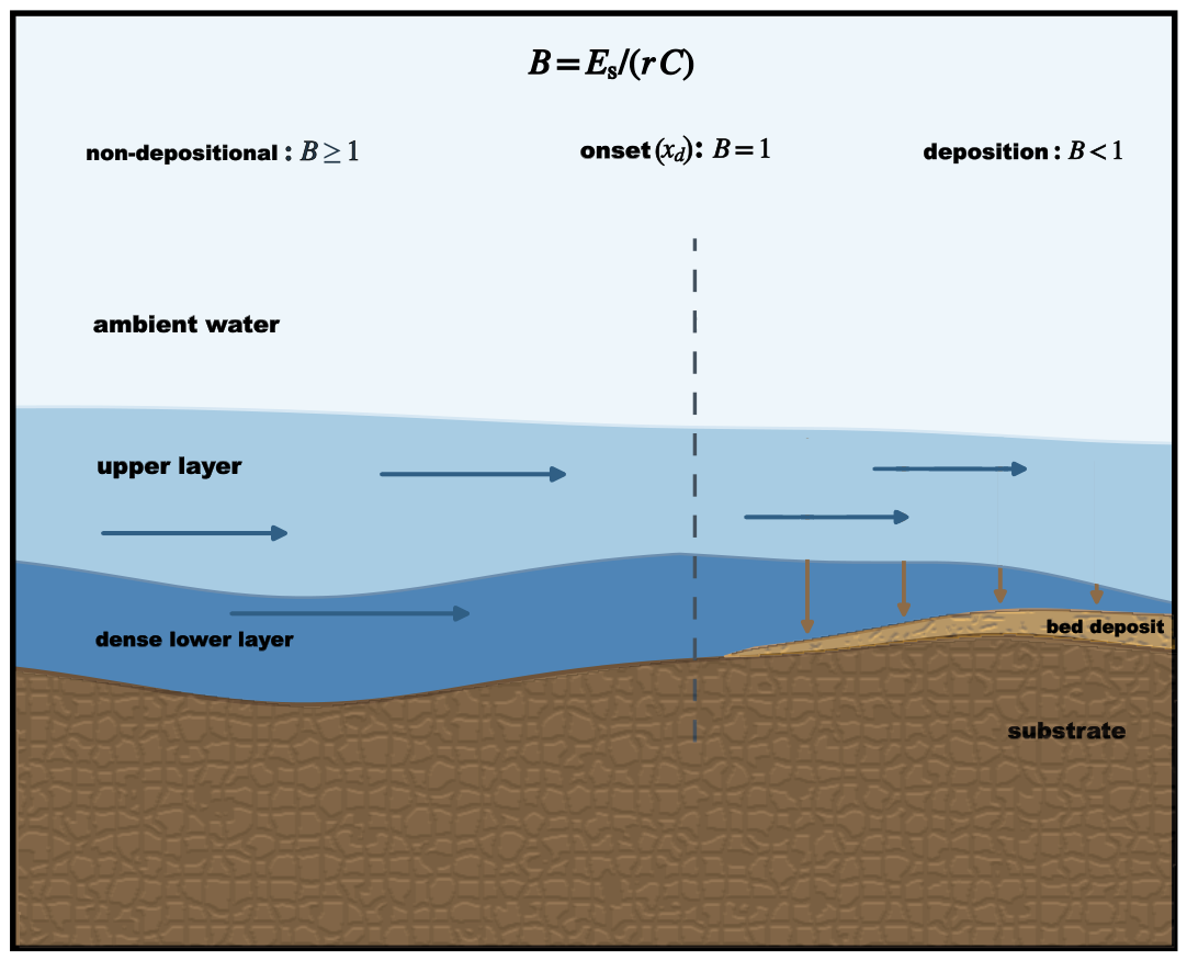
Figure 1 summarizes the conceptual structure of the reduced coupled framework.

3.3. Exact Coupled Evolution of B

Proposition 1.

Under (6)–(10), the state variable B satisfies the exact nonlinear evolution equation:

$${\displaystyle \frac{\mathrm{d}}{\mathrm{d}x}}logB=\mathcal{A}\left(x\right)-\Lambda \left(x\right)(B-1),$$

(11)

where

$$\mathcal{A}\left(x\right)=p{\displaystyle \frac{U_L^{\prime }}{U_L}}+{\displaystyle \frac{q_w^{\prime }}{q_w}}+\beta {\displaystyle \frac{e_{ws}^{\prime }}{e_{ws}}},$$

(12)

and

$$\Lambda \left(x\right)={\displaystyle \frac{v_s{r}_0}{q_w\left(x\right)}}.$$

(13)

Equivalently,

$${\displaystyle \frac{\mathrm{d}B}{\mathrm{d}x}}=\mathcal{A}\left(x\right)B-\Lambda \left(x\right)B(B-1).$$

(14)

Proof. 

Taking the logarithm of (9) and using the normalized closure (8) with constant $r_0$ gives

$${\displaystyle \frac{\mathrm{d}}{\mathrm{d}x}}logB=p{\displaystyle \frac{U_L^{\prime }}{U_L}}+\beta {\displaystyle \frac{e_{ws}^{\prime }}{e_{ws}}}-{\displaystyle \frac{C^{\prime }}{C}}.$$

From (6),

$$q_w{C}^{\prime }+q_w^{\prime }C=v_s(E_s-r_{0}C).$$

Dividing by $q_{w}C$ yields

$${\displaystyle \frac{C^{\prime }}{C}}={\displaystyle \frac{v_s}{q_w}}\left({\displaystyle \frac{E_s}{C}}-r_0\right)-{\displaystyle \frac{q_w^{\prime }}{q_w}}.$$

Since $E_s/C=r_{0}B$, this becomes

$${\displaystyle \frac{C^{\prime }}{C}}=\Lambda \left(x\right)(B-1)-{\displaystyle \frac{q_w^{\prime }}{q_w}}.$$

Substituting into the logarithmic derivative of B gives (11), and multiplication by B gives (14). □

Equation (14) is the exact coupled evolution law for B on the prescribed background. The first term, $\mathcal{A}\left(x\right)B$, is the same structural competition captured by the leading-order criterion. The second term, $-\Lambda \left(x\right)B(B-1)$, is the suspended-load feedback generated by finite bed exchange. When $B>1$, this term pushes B downward and therefore promotes earlier return toward onset; when $B<1$, it opposes further departure below unity.

It is convenient to define the first onset of deposition as

$$x_d=inf\{x>0:B\left(x\right)=1\mathrm{and}B\left(\xi \right)>1\mathrm{for}0<\xi <x\}.$$

(15)

The onset problem is therefore no longer purely algebraic: in the prescribed-background coupled theory it is the first return of the nonlinear state variable B to unity. For the Amazon-like backgrounds considered below, the upstream drift is initially positive, so both the leading-order and exact solutions first enter a non-depositional branch ($B>1$) before returning to unity. The onset definition in (15) should be read in that sense.

3.4. Weak-Exchange Expansion and the Leading-Order Criterion

An algebraic onset criterion appears naturally as a weak-exchange limit of (14). Introduce a bookkeeping parameter $\epsilon \ll 1$ by writing

$$\Lambda \left(x\right)=\epsilon \lambda \left(x\right),$$

(16)

and seek

$$B\left(x\right)=B_0\left(x\right)+\epsilon B_1\left(x\right)+O\left({\epsilon }^2\right).$$

(17)

At leading order,

$${\displaystyle \frac{\mathrm{d}{B}_0}{\mathrm{d}x}}=\mathcal{A}\left(x\right)B_0,B_0\left(0\right)=1,$$

(18)

so that

$$B_0\left(x\right)={\left({\displaystyle \frac{U_L\left(x\right)}{U_{L0}}}\right)}^p\left({\displaystyle \frac{q_w\left(x\right)}{q_{w0}}}\right){\left({\displaystyle \frac{e_{ws}\left(x\right)}{e_{ws,0}}}\right)}^{\beta }.$$

(19)

This is the leading-order algebraic onset criterion used throughout the reduced analysis.

At first order,

$${\displaystyle \frac{\mathrm{d}{B}_1}{\mathrm{d}x}}-\mathcal{A}\left(x\right)B_1=-\lambda \left(x\right)B_0\left(x\right)\left(B_0\left(x\right)-1\right),B_1\left(0\right)=0,$$

(20)

with solution

$$B_1\left(x\right)=-B_0\left(x\right){\int }_0^x\lambda \left(\xi \right)\left(B_0\left(\xi \right)-1\right)\mathrm{d}\xi .$$

(21)

Whenever $B_0>1$ upstream of onset, the first-order correction is negative. The weak-exchange expansion therefore already suggests that finite exchange favours an upstream shift of the onset relative to the leading-order estimate.

Corollary 1.

In the weak-exchange limit, the leading-order onset location $x_d^{\left(0\right)}$ is the first downstream return of $B_0$ to unity,

$$x_d^{\left(0\right)}=inf\{x>0:B_0\left(x\right)=1and{B}_0\left(\xi \right)>1\mathit{for}0<\xi <x\}.$$

(22)

At fixed downstream location x with $e_{ws}\left(x\right)<e_{ws,0}$, the corresponding pointwise threshold is

$${\beta }_{*}^{\left(0\right)}(x;p)={\displaystyle \frac{ln\left[\left(q_w\left(x\right)/q_{w0}\right){\left(U_L\left(x\right)/U_{L0}\right)}^p\right]}{ln\left[e_{ws,0}/e_{ws}\left(x\right)\right]}},$$

(23)

and the interval threshold is

$${\beta }_{\mathrm{crit}}^{\left(0\right)}(p;L)=\underset{0<x\le L}{inf}{\beta }_{*}^{\left(0\right)}(x;p).$$

(24)

We distinguish the pointwise threshold ${\beta }_{*}^{\left(0\right)}(x;p)$ from the interval threshold ${\beta }_{\mathrm{crit}}^{\left(0\right)}(p;L)$, the latter being the cumulative infimum over $0<x\le L$. The interval threshold is used below to construct the Amazon-like threshold curves.

3.5. Linearization of the Exact Coupled Equation and Comparison with the Leading-Order Solution

The Riccati form (14) can be linearized exactly by introducing the reciprocal variable

$$Y\left(x\right)={\displaystyle \frac{1}{B\left(x\right)}}.$$

(25)

Since $B\left(0\right)=1$, the transformed variable satisfies $Y\left(0\right)=1$. Substituting (25) into (14) gives the linear first-order equation

$${\displaystyle \frac{\mathrm{d}Y}{\mathrm{d}x}}+\left(\mathcal{A}\left(x\right)+\Lambda \left(x\right)\right)Y=\Lambda \left(x\right).$$

(26)

Proposition 2.

Let

$$I\left(x\right)={\int }_0^x\left(\mathcal{A}\left(\xi \right)+\Lambda \left(\xi \right)\right)\mathrm{d}\xi ,L\left(x\right)={\int }_0^x\Lambda \left(\xi \right)\mathrm{d}\xi .$$

(27)

Then, the exact coupled solution of (14) with $B\left(0\right)=1$ is

$$Y\left(x\right)=exp\left(-I\left(x\right)\right)\left[1+{\int }_0^x\Lambda \left(\xi \right)exp\left(I\left(\xi \right)\right)\mathrm{d}\xi \right],$$

(28)

or, equivalently,

$$B\left(x\right)={\displaystyle \frac{B_0\left(x\right)exp\left(L\left(x\right)\right)}{{\displaystyle 1+{\int }_0^x\Lambda \left(\xi \right)B_0\left(\xi \right)exp\left(L\left(\xi \right)\right)\mathrm{d}\xi }}},$$

(29)

where $B_0$ is the leading-order weak-exchange solution given by (19).

Proof. 

Equation (26) is linear. Multiplying by the integrating factor

$$exp\left(I\left(x\right)\right)=exp\left({\int }_0^x\left(\mathcal{A}\left(\xi \right)+\Lambda \left(\xi \right)\right)\mathrm{d}\xi \right)$$

gives

$${\displaystyle \frac{\mathrm{d}}{\mathrm{d}x}}\left(Y\left(x\right)exp\left(I\left(x\right)\right)\right)=\Lambda \left(x\right)exp\left(I\left(x\right)\right).$$

Integrating from 0 to x and using $Y\left(0\right)=1$ yields (28). Since

$$B_0\left(x\right)=exp\left({\int }_0^x\mathcal{A}\left(\xi \right)\mathrm{d}\xi \right),$$

we have

$$exp\left(I\left(x\right)\right)=B_0\left(x\right)exp\left(L\left(x\right)\right),$$

and (29) follows after taking the reciprocal. □

The transformed form (26) makes clear that the exact coupled problem is analytically more structured than the Riccati form alone suggests. It also yields a sharper comparison with the leading-order solution.

Proposition 3.

Assume that the leading-order solution satisfies

$$B_0\left(x\right)\ge 1\mathit{for}\mathit{all}x\in [0,L].$$

(30)

Then the exact coupled solution satisfies

$$B\left(x\right)\le B_0\left(x\right)\mathit{for}\mathit{all}x\in [0,L].$$

(31)

Consequently, if the leading-order onset location $x_d^{\left(0\right)}$ exists, then the exact prescribed-background coupled onset satisfies

$$x_d\le x_d^{\left(0\right)}.$$

(32)

Proof. 

Let

$$Y_0\left(x\right)={\displaystyle \frac{1}{B_0\left(x\right)}}.$$

Since $B_0$ solves (18), the reciprocal $Y_0$ satisfies

$${\displaystyle \frac{\mathrm{d}{Y}_0}{\mathrm{d}x}}+\mathcal{A}\left(x\right)Y_0=0,Y_0\left(0\right)=1.$$

(33)

Define $D\left(x\right)=Y\left(x\right)-Y_0\left(x\right)$. Subtracting (33) from (26) gives

$${\displaystyle \frac{\mathrm{d}D}{\mathrm{d}x}}+\left(\mathcal{A}\left(x\right)+\Lambda \left(x\right)\right)D=\Lambda \left(x\right)\left(1-Y_0\left(x\right)\right),D\left(0\right)=0.$$

(34)

Under (30), one has $Y_0\left(x\right)\le 1$, so the right-hand side of (34) is non-negative. By the integrating-factor formula, $D\left(x\right)\ge 0$ for all $x\in [0,L]$. Therefore,

$$Y\left(x\right)\ge Y_0\left(x\right),$$

which implies

$$B\left(x\right)\le B_0\left(x\right).$$

If $x_d^{\left(0\right)}$ is the first downstream return of $B_0$ to unity, then continuity and (31) imply that the exact coupled solution can only reach $B=1$ earlier or at the same point. Hence, (32) follows. □

Proposition 3 strengthens the weak-exchange interpretation: finite suspended-load exchange does not merely perturb the leading-order threshold, but shifts the exact solution below the leading-order one throughout any reach on which the leading-order state remains non-depositional. The upstream shift of depositional onset is therefore not only asymptotic but exact on that interval.

Remark 1.

If the near-bed concentration ratio were allowed to vary downstream, $r=r\left(x\right)$, then the exact drift term would acquire an additional contribution $-r^{\prime }/r$ inside $\mathcal{A}\left(x\right)$. Here, $r=r_0$ is kept fixed in order to isolate the effect of suspended-load coupling itself. Exact coupled applications are therefore reported below in terms of the effective exchange-strength parameter ${\Lambda }_0$ rather than as a calibration of $r_0$.

4. Amazon-like Application and Computational Workflow

The calculations in this section are used as an illustrative reduced-model benchmark. Their purpose is to show how the state-variable theory behaves on an Amazon-like long-runout background and to test sensitivity to exchange strength, closure choice, inlet state, grid resolution and background perturbations. They should not be read as a site-specific prediction of the Amazon system or as a full reproduction of the parent two-layer solver.

4.1. Prescribed Background and Reproducibility

The Amazon-like application uses the exponentially decaying bed slope adopted by Ma et al. [17],

$$S\left(x\right)=S_{u}exp(-x/x_e),S_u=0.0166,x_e=265.8\mathrm{km}.$$

(35)

The representative parent-state parameters are

$$q_{w0}=100{\mathrm{m}}^2{\mathrm{s}}^{-1},q_s=0.6{\mathrm{m}}^2{\mathrm{s}}^{-1},C_{fb}=0.002,D=62.5\mu \mathrm{m}.$$

(36)

In the full two-layer calculation of Ma et al. [17], the lower layer remains supercritical until approximately $x=402$ km, while the downstream lower-layer water flux reaches a maximum near $x=328$ km. These distances remain the natural morphodynamic targets.

The computational pipeline used here is explicit. The prescribed Amazon-like background is distributed in the reproducibility package as a gridded imported background and, for convenience, as self-contained surrogate functions for the ratios $U_L/U_{L0}$, $q_w/q_{w0}$ and $e_{ws}/e_{ws,0}$ on $0\le x\le 400$ km. These surrogate functions reproduce the background used in the reduced calculations; they do not replace a full parent-solver evaluation. In physical terms, the background represents a local-normal-flow reconstruction of the parent two-layer branch: the local slope $S\left(x_i\right)$ from (35) selects pointwise values of $U_{Ln}$, $q_{wn}$ and $e_{ws,n}$, which are then normalized by their upstream values. In the distributed scripts the same information is used through a tabulated file, including the upstream reference point $x=0$, and samples every 1 km to 400 km. The exact-coupled curves are initialized with the upstream condition $B\left(0\right)=1$ and then reported on the same downstream grid used for the prescribed background. The resulting CSV files included in the submission package provide the imported ratios together with derived leading-order and exact-coupled quantities. The gridded data and Python scripts used for these calculations are provided as File S1 in the Supplementary Materials. The representative ratios at the two target distances are

$${\displaystyle \frac{U_L\left(328\mathrm{km}\right)}{U_{L0}}}\approx 0.799,{\displaystyle \frac{q_w\left(328\mathrm{km}\right)}{q_{w0}}}\approx 6.75,{\displaystyle \frac{e_{ws}\left(328\mathrm{km}\right)}{e_{ws,0}}}\approx 0.544,$$

(37)

and

$${\displaystyle \frac{U_L\left(400\mathrm{km}\right)}{U_{L0}}}\approx 0.776,{\displaystyle \frac{q_w\left(400\mathrm{km}\right)}{q_{w0}}}\approx 6.09,{\displaystyle \frac{e_{ws}\left(400\mathrm{km}\right)}{e_{ws,0}}}\approx 0.492.$$

(38)

These ratios are the prescribed background used in all downstream calculations. All crossing locations reported in the onset tables below are extracted from the first sign change of $B_0-1$ or $B-1$ by linear interpolation between the neighbouring grid points. Whenever a curve is continued beyond its first onset, that continuation should be interpreted according to the governing equation used: for $B_0$ it is a diagnostic continuation of the weak-exchange background; for B it is the exact reduced evolution on the prescribed hydrodynamic background. Linear interpolation on the gridded background gives the weak-exchange onset $x_d^{\left(0\right)}\approx 379.7$ km.

Because the full downstream integration code of the parent calculation is not part of the present reduced package, the reconstruction is checked in two more limited ways. First,

Table 1. Fidelity check of the local-normal-flow reconstruction against diagnostic values reported for the parent Amazon-like calculation. The comparison is deliberately limited to published parent-output quantities and is not a full-solver validation.

Diagnostic	Parent Value	Reconstruction	Comment
position of maximum $q_w$	328 km	328 km	matched anchor
maximum $q_w$	$675{\mathrm{m}}^2{\mathrm{s}}^{-1}$	$675{\mathrm{m}}^2{\mathrm{s}}^{-1}$	matched anchor
$U_L$ at 400 km	about $2.14\mathrm{m}{\mathrm{s}}^{-1}$	$2.13\mathrm{m}{\mathrm{s}}^{-1}$	within $1\%$
${\delta }_L$ at 200 km	about 250 m	about 224 m	about $10\%$ low

compares the local-normal-flow background with diagnostic values reported for the parent Amazon-like case. This is a fidelity check against published parent-output metrics, not a substitute for a full code-to-code validation. Secondly, the perturbation analysis reported below propagates representative downstream-ramped perturbations of the imported fields into the onset location. The largest tested perturbation of $e_{ws}$ shifts the representative onset by about 14 km, so the quoted onset distances should be read as reduced-model estimates rather than field-calibrated predictions.

4.2. Leading-Order Threshold Curves

Applying (24) to the gridded Amazon-like background yields the interval thresholds

$${\beta }_{\mathrm{crit}}^{\left(0\right)}(p;400\mathrm{km})\approx 2.19(p=1),1.83(p=2),1.47(p=3),$$

(39)

and

$${\beta }_{\mathrm{crit}}^{\left(0\right)}(p;328\mathrm{km})\approx 2.77(p=1),2.40(p=2),2.03(p=3).$$

(40)

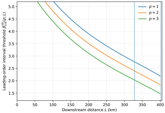
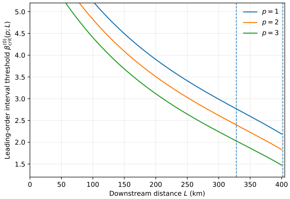
The curves in Figure 2 show the corresponding interval-threshold curves for $p=1,2,3$. Because ${\beta }_{\mathrm{crit}}^{\left(0\right)}(p;L)$ is defined as a cumulative infimum, the curves are monotone non-increasing by construction. They therefore summarize the minimum stratification sensitivity required for the leading-order onset to occur before a prescribed distance.

The threshold values are listed in

Table 2. Leading-order interval thresholds in the Amazon-like application.

Shear Exponent p	${\mathit{\beta }}_{\mathbf{crit}}^{\left(0\right)}(\mathit{p};328\mathbf{km})$	${\mathit{\beta }}_{\mathbf{crit}}^{\left(0\right)}(\mathit{p};400\mathbf{km})$
1	2.77	2.19
2	2.40	1.83
3	2.03	1.47

. Consistent with the algebraic structure of (23), the threshold decreases with increasing p: if entrainment is already strongly shear-sensitive, less additional suppression through interfacial stratification is required in the weak-exchange limit.

4.3. Leading-Order Diagnostic Continuations

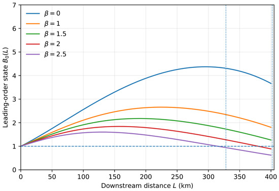
The curves in Figure 3 show the leading-order curves $B_0\left(L\right)$ for $p=2$ and several values of $\beta$. The dashed horizontal line marks $B_0=1$. In the weak-exchange approximation, the shear-only case $\beta =0$ remains well above unity throughout the pre-critical reach, mild suppression ($\beta =1$ or $1.5$) weakens but does not eliminate this non-depositional behaviour, while $\beta \gtrsim 2$ produces a leading-order onset before the Froude-critical transition.

The leading-order crossing distances are listed in

Table 3. Leading-order onset estimates for $p=2$ on the prescribed Amazon-like background.

$\mathit{\beta }$	Leading-Order ${\mathit{x}}_{\mathit{d}}^{\left(0\right)}$ (km)	${\mathit{B}}_0\left(328\mathbf{km}\right)$	${\mathit{B}}_0\left(400\mathbf{km}\right)$
0.0	no onset before 400	4.31	3.67
1.0	no onset before 400	2.34	1.80
1.5	no onset before 400	1.73	1.27
2.0	379.7	1.28	0.89
2.5	314.9	0.94	0.62

. They remain useful as weak-exchange benchmarks even after exact suspended-load coupling is included, because they show how strongly the onset location responds to $\beta$ before feedback through the exchange term is taken into account.

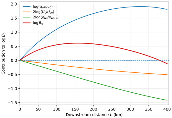
The decomposition in Figure 4 separates $log{B}_0$ for the representative case $p=2$, $\beta =2$. The positive term $log(q_w/q_{w0})$ is largest in the upstream and mid-reach because increasing lower-layer water flux dilutes the concentration. The negative contributions associated with velocity decay and interfacial suppression accumulate more gradually, but eventually dominate and drive $log{B}_0$ below zero. This remains the clearest reduced picture of the onset mechanism even after exact suspended-load coupling is included.

4.4. Exact Coupled Evolution on the Prescribed Background

The exact prescribed-background coupled calculation introduces one additional exchange-strength parameter,

$${\Lambda }_0={\displaystyle \frac{{10}^3{v}_s{r}_0}{q_{w0}}},$$

(41)

when x is measured in kilometres. Then,

$$\Lambda \left(x\right)={\Lambda }_0{\displaystyle \frac{q_{w0}}{q_w\left(x\right)}}.$$

(42)

Physically, $\Lambda$ compares the local settling/exchange scale $v_s{r}_0$ with the downstream advective water flux $q_w$. Small ${\Lambda }_0$ corresponds to a weak-exchange regime close to the algebraic limit; larger ${\Lambda }_0$ increases the feedback term $-\Lambda B(B-1)$ and therefore accelerates the return of B toward the depositional threshold. Because $r_0$ is not independently calibrated in the present reduced study, the coupled application is reported parametrically in terms of ${\Lambda }_0$.

For the representative grain size $D=62.5$ μm, the settling speed used in the reduced application is of order $v_s\approx 3.5\times {10}^{-3}\mathrm{m}{\mathrm{s}}^{-1}$. With $q_{w0}=100{\mathrm{m}}^2{\mathrm{s}}^{-1}$, this gives

$${\Lambda }_0\approx 0.035r_0{\mathrm{km}}^{-1}.$$

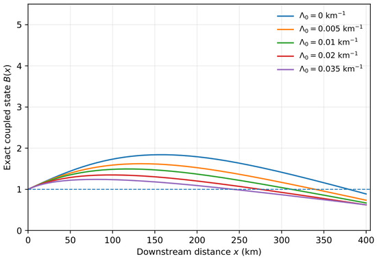
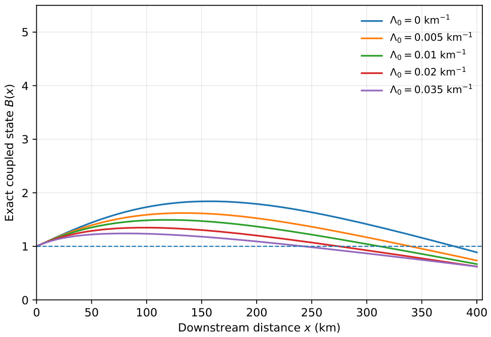
The non-zero illustrative range used in Figure 5, namely ${\Lambda }_0=0.005$–$0.035{\mathrm{km}}^{-1}$, should therefore be read as a sensitivity range from weak exchange to moderate exchange in an Amazon-like setting, not as a direct calibration of $r_0$. The additional case ${\Lambda }_0=0$ is shown only as the exact weak-exchange limit. The lower non-zero end of the range is a small feedback perturbation, while the upper end corresponds to order-unity values of the near-bed concentration ratio.

The curves in Figure 5 show exact prescribed-background coupled solutions of (14) for the representative case $p=2$, $\beta =2$ and selected values of ${\Lambda }_0$. The curve with ${\Lambda }_0=0$ is the exact weak-exchange limit evaluated on the same gridded background and therefore coincides pointwise with the leading-order solution $B_0$. As ${\Lambda }_0$ increases, the additional feedback term $-\Lambda B(B-1)$ drives the solution back toward onset more quickly, shifting deposition upstream. This is the clearest quantitative consequence of restoring suspended-load consistency.

The exact onset locations shown in Figure 5 are summarized in

Table 4. Exact coupled onset locations for the representative case $p=2$, $\beta =2$. The ${\Lambda }_0=0$ row is the exact weak-exchange limit and coincides with the leading-order solution evaluated on the same grid.

${\mathbf{\Lambda }}_0$ (km−1)	Exact Onset ${\mathit{x}}_{\mathit{d}}$ (km)	$\mathit{B}$ (400 km)
0.000	379.7	0.888
0.005	339.9	0.736
0.010	311.9	0.669
0.020	275.0	0.623
0.035	243.1	0.624

. Even modest exchange strengths produce substantial upstream shifts relative to the interpolated weak-exchange value $x_d^{\left(0\right)}\approx 379.7$ km. The curve with ${\Lambda }_0=0$ is evaluated on the same gridded background and therefore gives the same onset reported in Table 4.

4.5. Grid Convergence and Robustness Checks

The onset locations are extracted by linear interpolation on gridded curves. The grid-refinement test in

Table 5. Grid-refinement check for the representative exact prescribed-background coupled calculation with $p=2$, $\beta =2$. Entries are onset locations $x_d$ in km.

$\mathbf{\Delta }\mathit{x}$ (km)	${\mathbf{\Lambda }}_0=0$	$0.005$	$0.010$	$0.020$	$0.035$
1.00	379.716	339.938	311.910	274.970	243.092
0.50	379.716	339.937	311.908	274.967	243.089
0.25	379.716	339.937	311.908	274.967	243.088

reports a simple grid-refinement check for the representative case $p=2$, $\beta =2$. The changes between $\Delta x=1$, $0.5$ and $0.25$ km are below $0.01$ km for the weak-exchange row and below $0.01$–$0.003$ km for the exact coupled rows shown here. The tenths of kilometres reported in Table 3 and Table 4 are therefore controlled by the reduced background itself, not by grid resolution.

The perturbation results in

Table 6. Sensitivity of the representative exact prescribed-background coupled onset $(p=2,\beta =2,$ ${\Lambda }_0=0.01{\mathrm{km}}^{-1})$ to downstream-ramped perturbations of the imported background fields.

Perturbation	${\mathit{x}}_{\mathit{d}}$ (km)	Shift from Baseline (km)
baseline	311.91	0.00
$U_L$ ramp $-2\%$	306.11	$-5.80$
$U_L$ ramp $+2\%$	317.64	$+5.73$
$q_w$ ramp $-5\%$	303.82	$-8.09$
$q_w$ ramp $+5\%$	319.79	$+7.88$
$e_{ws}$ ramp $-5\%$	297.32	$-14.58$
$e_{ws}$ ramp $+5\%$	326.10	$+14.20$

give a small uncertainty budget for the prescribed background. Each perturbation is applied as a downstream-ramped multiplicative perturbation that is zero at the inlet and reaches the stated amplitude at 400 km. The amplitudes are deliberately small to moderate: $\pm 2\%$ for $U_L$ and $\pm 5\%$ for $q_w$ and $e_{ws}$. These values are not calibrated uncertainty bounds; they are stress tests of the prescribed-background approximation. They are large enough to change the onset location by several kilometres, but small enough to preserve the qualitative structure of the imported background. This does not replace validation against the full parent solver, but it quantifies how sensitive the representative onset is to plausible background-reconstruction errors.

Two further checks delimit the dependence on the closure and inlet normalization. First, replacing the power-law stratification factor ${(e_{ws}/e_{ws,0})}^{\beta }$ by the alternative normalized factor $exp[-\gamma (1-e_{ws}/e_{ws,0})]$, with $\gamma$ chosen so that the suppression at 400 km matches the $\beta =2$ power-law case, gives $x_d\approx 311.1$ km for ${\Lambda }_0=0.01{\mathrm{km}}^{-1}$, compared with $311.9$ km for the power-law closure. Secondly, for the same parameter values, changing the inlet state from $B_{\mathrm{in}}=1$ to $B_{\mathrm{in}}=1.1$ shifts the exact onset to $318.6$ km, while $B_{\mathrm{in}}=0.9$ is already depositional at the inlet. These checks show that the reduced theory is not tied to a unique algebraic normalization, although quantitative onset locations remain closure- and inlet-dependent.

5. Discussion

5.1. Scope of the Coupled Reduced Theory

The framework separates three levels of description. The prescribed two-layer bypass background is inherited from the parent theory of Ma et al. [17]. On that background, suspended-sediment evolution and Exner exchange are coupled exactly through (6) and (14). The algebraic threshold ${\beta }_{\mathrm{crit}}^{\left(0\right)}$ is then a leading-order consequence of that coupled reduced theory in the weak-exchange limit.

This separation also defines the scope of the model. The theory is coupled in suspended load and bed exchange, but not yet fully hydro-morphodynamic. The hydrodynamic fields $U_L\left(x\right)$, $q_w\left(x\right)$ and $e_{ws}\left(x\right)$ are prescribed from a long-runout bypass background. A fully hydro-morphodynamic theory would let the evolving bed feed back onto those fields. The framework is therefore best described as a coupled reduced theory on a prescribed two-layer bypass background.

5.2. Regime of Validity of the Prescribed-Background Approximation

The theory is exact only for suspended load and bed exchange on a prescribed hydrodynamic background. Its use over the pre-onset reach assumes that cumulative aggradation or degradation remains asymptotically small compared with the local layer thicknesses and that the morphodynamic slope generated by $\eta \left(x\right)$ remains small compared with the imposed downstream variation already built into $S\left(x\right)$. In that regime the imported fields $U_L\left(x\right)$, $q_w\left(x\right)$ and $e_{ws}\left(x\right)$ evolve primarily because of the prescribed two-layer hydraulics, while bed exchange acts as a one-way perturbation on the suspended load. Once deposition persists over longer reaches, or once bed relief becomes comparable with the local layer thickness, feedback onto the background hydrodynamics can no longer be neglected and the present reduced theory should be replaced by a fully two-way hydro-morphodynamic calculation.

5.3. Physical Interpretation

The physical message of the theory is that the leading-order drift term $\mathcal{A}\left(x\right)$ expresses the three-way competition among lower-layer deceleration, downstream dilution through $q_w$, and stratification-sensitive suppression of $e_{ws}$. The exact coupled correction does not replace that competition; it modifies it through the nonlinear restoring term $-\Lambda B(B-1)$. On any reach over which the leading-order solution remains non-depositional, the exact coupled solution lies below the leading-order one, so finite exchange favours an upstream shift of depositional onset.

The leading-order criterion remains useful because it isolates the structural competition among $U_L$, $q_w$ and $e_{ws}$ in closed form. The coupled evolution then quantifies how much additional upstream shift is introduced once suspended-sediment exchange with the bed is retained.

This interpretation is also consistent with recent monitoring and deposit-based studies, which show that process and preserved stratigraphy need not map one-to-one. Dense heads can control sediment flux and runout [21], direct monitoring provides increasingly detailed constraints on active turbidity-current structure [22,23], and deposit-centred analyses show that actual turbidite preservation can be incomplete or strongly filtered by the dynamics of individual flows [30,31]. The reduced threshold proposed here should therefore be read as a process-level criterion for onset, not as a complete inversion rule from deposits alone.

5.4. Limitations and Next Steps

Several limitations remain explicit. First, the local-normal-flow reconstruction is a surrogate for the full parent solver. Here, the reconstruction is checked against reported parent-output diagnostics and perturbation sensitivities, but no full code-to-code validation is claimed. Secondly, a single grain-size class is represented through a single settling velocity, bedload is neglected at leading order, and $r=r_0$ is held constant. Thirdly, the stratification dependence in (8) is intentionally minimal; $\beta$ should be interpreted as an effective sensitivity parameter unless a stronger transport closure is established. Finally, the prescribed-background-coupled application is reported parametrically in ${\Lambda }_0$ because the constant-$r_0$ closure is not yet calibrated independently.

These limitations point directly to the next steps. The most immediate extension is to insert the same suspended-sediment balance into the full two-layer equations solved by Ma et al. [17]. A second step is to allow several grain classes, in which case the analogue of B becomes class-dependent. A third step is to relax the prescribed-background assumption and let the evolving bed feed back onto the hydrodynamic fields themselves. Even in those fuller settings, however, the prescribed-background reduced Equation (14) and its weak-exchange limit should remain useful because they isolate the onset mechanism in a form that can be analysed directly.

6. Conclusions

A reduced morphodynamic extension of the two-layer long-runout theory of Ma et al. [17] has been developed so that suspended load and bed exchange are coupled consistently on a prescribed bypass background. The general theoretical conclusions and the Amazon-like illustrative results should be kept distinct. The main findings are as follows.

1.

The state variable $B=E_s/\left(rC\right)$ satisfies an exact nonlinear evolution equation on the prescribed two-layer background. The missing suspended-sediment source term can therefore be retained without abandoning a reduced analytical framework.

2.

The algebraic criterion is recovered as the weak-exchange limit of the exact coupled equation. In that limit, the threshold ${\beta }_{\mathrm{crit}}^{\left(0\right)}(p;L)$ remains a useful leading-order summary of the onset problem.

3.

In the illustrative Amazon-like background, finite exchange shifts depositional onset upstream relative to the leading-order estimate. This is a model-dependent numerical result, but it follows the general comparison principle that, on any reach over which the leading-order solution remains non-depositional, the exact prescribed-background coupled solution lies below the leading-order one.

4.

The framework is coupled in suspended load and bed exchange, but it remains reduced at the hydrodynamic level. Its proper role is therefore that of a coupled reduced theory on a prescribed two-layer bypass background, not a fully hydro-morphodynamic closure. The Amazon-like numerical values should be read together with the reported background-fidelity, convergence and closure-sensitivity checks.

References

- Kneller, B.; Buckee, C. The structure and fluid mechanics of turbidity currents: A review of some recent studies and their geological implications. Sedimentology 2000, 47, 62–94. [Google Scholar] [CrossRef] [Scilit]
- Meiburg, E.; Kneller, B. Turbidity currents and their deposits. Annu. Rev. Fluid Mech. 2010, 42, 135–156. [Google Scholar] [CrossRef] [Scilit]
- Wells, M.G.; Dorrell, R.M. Turbulence processes within turbidity currents. Annu. Rev. Fluid Mech. 2021, 53, 59–83. [Google Scholar] [CrossRef] [Scilit]
- Talling, P.J.; Baker, M.L.; Pope, E.L.; Ruffell, S.C.; Jacinto, R.S.; Heijnen, M.S.; Hage, S.; Simmons, S.M.; Hasenhündl, M.; Heerema, C.J.; et al. Longest sediment flows yet measured show how major rivers connect efficiently to deep sea. Nat. Commun. 2022, 13, 4193. [Google Scholar] [CrossRef] [Scilit]
- Baker, M.L.; Pope, E.L.; Talling, P.J.; Burnett, R.; Ruffell, S.C.; Hage, S.; Jacinto, R.S.; Heijnen, M.S.; Urlaub, M.; Clare, M.A.; et al. Seabed seismographs reveal duration and structure of longest runout sediment flows on Earth. Geophys. Res. Lett. 2024, 51, e2024GL111078. [Google Scholar] [CrossRef] [Scilit]
- Paull, C.K.; Talling, P.J.; Maier, K.L.; Parsons, D.; Xu, J.; Caress, D.W.; Gwiazda, R.; Lundsten, E.M.; Anderson, K.; Barry, J.P.; et al. Powerful turbidity currents driven by dense basal layers. Nat. Commun. 2018, 9, 4114. [Google Scholar] [CrossRef] [Scilit]
- Wang, Z.; Xu, J.; Talling, P.J.; Cartigny, M.J.B.; Simmons, S.M.; Gwiazda, R.; Paull, C.K.; Maier, K.L.; Parsons, D.R. Direct evidence of a high-concentration basal layer in a submarine turbidity current. Deep-Sea Res. Part I Oceanogr. Res. Pap. 2020, 161, 103300. [Google Scholar] [CrossRef] [Scilit]
- Kuenen, P.H.; Migliorini, C.I. Turbidity Currents as a Cause of Graded Bedding. J. Geol. 1950, 58, 91–127. [Google Scholar] [CrossRef] [Scilit]
- Middleton, G.V. Experiments on Density and Turbidity Currents: I. Motion of the Head. Can. J. Earth Sci. 1966, 3, 523–546. [Google Scholar] [CrossRef] [Scilit]
- Middleton, G.V. Experiments on Density and Turbidity Currents: II. Uniform Flow of Density Currents. Can. J. Earth Sci. 1966, 3, 627–637. [Google Scholar] [CrossRef] [Scilit]
- Lowe, D.R. Sediment Gravity Flows: II. Depositional Models with Special Reference to the Deposits of High-Density Turbidity Currents. J. Sediment. Petrol. 1982, 52, 279–297. [Google Scholar] [CrossRef] [Scilit]
- Middleton, G.V. Sediment Deposition from Turbidity Currents. Annu. Rev. Earth Planet. Sci. 1993, 21, 89–114. [Google Scholar] [CrossRef]
- Parker, G.; Fukushima, Y.; Pantin, H.M. Self-accelerating turbidity currents. J. Fluid Mech. 1986, 171, 145–181. [Google Scholar] [CrossRef] [Scilit]
- Naruse, H. A Review of the Autosuspension of Turbidity Currents: Its Significance and Gaps in Our Understanding. J. Geol. Soc. Jpn. 2011, 117, 122–132. [Google Scholar] [CrossRef] [Scilit]
- Talling, P.J.; Allin, J.; Armitage, D.A.; Arnott, R.W.C.; Cartigny, M.J.B.; Clare, M.A.; Felletti, F.; Covault, J.A.; Girardclos, S.; Hansen, E.; et al. Key Future Directions for Research on Turbidity Currents and Their Deposits. J. Sediment. Res. 2015, 85, 153–169. [Google Scholar] [CrossRef] [Scilit]
- Bolla Pittaluga, M.; Frascati, A.; Falivene, O. A Gradually Varied Approach to Model Turbidity Currents in Submarine Channels. J. Geophys. Res. Earth Surf. 2018, 123, 80–96. [Google Scholar] [CrossRef] [Scilit]
- Ma, H.; Parker, G.; Cartigny, M.; Viparelli, E.; Balachandar, S.; Fu, X.; Luchi, R. Two-layer formulation for long-runout turbidity currents: Theory and bypass flow case. J. Fluid Mech. 2025, 1009, A19. [Google Scholar] [CrossRef] [Scilit]
- Lippert, M.C.; Woods, A.W. Experiments on the sedimentation front in steady particle-driven gravity currents. J. Fluid Mech. 2020, 889, A20. [Google Scholar] [CrossRef] [Scilit]
- Tsai, Y.H.; Chou, Y.J. On the suspension and deposition within turbidity currents. J. Fluid Mech. 2025, 1003, A1. [Google Scholar] [CrossRef] [Scilit]
- Reece, J.K.; Dorrell, R.M.; Straub, K.M. Circulation of hydraulically ponded turbidity currents and the filling of continental slope minibasins. Nat. Commun. 2024, 15, 2075. [Google Scholar] [CrossRef] [Scilit]
- Pope, E.L.; Talling, P.J.; Carter, G.D.O.; Clare, M.A.; Hunt, J.E.; Cartigny, M.J.B.; Baker, M.L.; Pope, M.; Heijnen, M.S.; Simmons, S.M.; et al. First Source-to-Sink Monitoring Shows Dense Head Controls Sediment Flux and Runout in Turbidity Currents. Sci. Adv. 2022, 8, eabj3220. [Google Scholar] [CrossRef] [Scilit]
- Talling, P.J.; Cartigny, M.J.B.; Pope, E.L.; Baker, M.; Clare, M.A.; Heijnen, M.; Hage, S.; Parsons, D.R.; Simmons, S.M.; Paull, C.K.; et al. Detailed Monitoring Reveals the Nature of Submarine Turbidity Currents. Nat. Rev. Earth Environ. 2023, 4, 642–658. [Google Scholar] [CrossRef] [Scilit]
- Clare, M.A.; Lintern, D.G.; Rosenberger, K.; Hughes Clarke, J.E.; Paull, C.; Gwiazda, R.; Cartigny, M.J.B.; Talling, P.J.; Perara, D.; Xu, J.; et al. Lessons Learned from the Monitoring of Turbidity Currents and Guidance for Future Platform Designs. Geol. Soc. Lond. Spec. Publ. 2020, 500, 605–634. [Google Scholar] [CrossRef] [Scilit]
- Parker, G.; Garcia, M.; Fukushima, Y.; Yu, W. Experiments on turbidity currents over an erodible bed. J. Hydraul. Res. 1987, 25, 123–147. [Google Scholar] [CrossRef] [Scilit]
- Garcia, M.; Parker, G. Entrainment of bed sediment into suspension. J. Hydraul. Eng. 1991, 117, 414–435. [Google Scholar] [CrossRef] [Scilit]
- Garcia, M.; Parker, G. Experiments on the entrainment of sediment into suspension by a dense bottom current. J. Geophys. Res. Ocean. 1993, 98, 4793–4807. [Google Scholar] [CrossRef] [Scilit]
- Huppert, H.E.; Turner, J.S.; Hallworth, M.A. Sedimentation and Entrainment in Dense Layers of Suspended Particles Stirred by an Oscillating Grid. J. Fluid Mech. 1995, 289, 263–293. [Google Scholar] [CrossRef] [Scilit]
- Shringarpure, M.; Cantero, M.I.; Balachandar, S. Dynamics of Complete Turbulence Suppression in Turbidity Currents Driven by Monodisperse Suspensions of Sediment. J. Fluid Mech. 2012, 712, 384–417. [Google Scholar] [CrossRef] [Scilit]
- Huang, R.; Zhang, Q.; Zhang, W.; Li, Z. Experimental Research on the Effect of Suspended Sediment Stratification on Turbulence Characteristics. Estuar. Coast. Shelf Sci. 2022, 278, 108128. [Google Scholar] [CrossRef] [Scilit]
- Ge, Z.; Nemec, W.; Vellinga, A.J.; Gawthorpe, R.L. How Is a Turbidite Actually Deposited? Sci. Adv. 2022, 8, eabl9124. [Google Scholar] [CrossRef] [Scilit] [PubMed]
- Jacques, F.; Normandeau, A.; Montero-Serrano, J.C.; St-Onge, G.; Limoges, A.; Rochon, A.; Neumeier, U.; Lajeunesse, P.; Bourgault, D. The Incompleteness of Turbidite Records: Comparing Direct Monitoring of Turbidity Currents to Deposits Preserved in Submarine Fans (Pointe-des-Monts, Eastern Canada). Mar. Geol. 2025, 491, 107660. [Google Scholar] [CrossRef] [Scilit]
Disclaimer/Publisher’s Note: The statements, opinions and data contained in all publications are solely those of the individual author(s) and contributor(s) and not of MDPI and/or the editor(s). MDPI and/or the editor(s) disclaim responsibility for any injury to people or property resulting from any ideas, methods, instructions or products referred to in the content. |
© 2026 by the author. Licensee MDPI, Basel, Switzerland. This article is an open access article distributed under the terms and conditions of the Creative Commons Attribution (CC BY) license.