Abstract
This paper uses the flexural vibration of cantilever beams as a benchmark problem to test mesh-free and finite element methods in structural dynamics. First, a symbolic analysis of the “kernel collocation” type mesh-free method is carried out, in which the collocation function satisfies the boundary conditions. This enables both Finite Element (FE) and mesh-free results to be compared with exact analytical ones. Thereafter, the natural frequencies and Frequency Response Function (FRF), in terms of the beam parameters, are determined and compared with the analytical results, that exist in the literature. It is shown that by adjusting the parameters of the kernel function, we can find identical peaks to those of the analytical method. The finite element method is also employed to solve this problem, and the first three natural frequencies were computed in terms of the beam parameters. When comparing the two methods, we see that by increasing the number of elements in the FEM we can always achieve better accuracy, but we will obtain twice the number of modal frequencies. However, the mesh-free method with the same number of nodes does not provide these extra frequencies. From this benchmark problem, it is concluded that the accuracy of the mesh-free methods always depends on the adjustment of the kernel function. However, the FEM is advantageous because it does not require such adjustments.
1. Introduction
Mesh-free methods have been used to solve problems in science and engineering since the early 1990s. The field remained active in structural dynamics and vibration because of its advantages versus the Finite Element Method (FEM). In the FEM for accuracy, it is required to increase the number of elements, thereby the number of Degrees Of Freedom (DOF) rises that result in substantial numbers of natural frequencies, and particular techniques are required to refine the unnecessary modes.
As indicated recently in [1], for shell-type structures a mesh-free method is capable of producing fundamental modes accurately. Moreover, in diverse support conditions with various boundary conditions, the mesh-free methods in structural vibrations are also useful as shown in [2]. Moreover, the versatility of the method in 1D and 2D structural vibration models has been proved and commented upon in [3]. It should be noted that a substantial literature survey was also conducted in [1,2,3] that justifies research to investigate the accuracy and sensitivity of these methods when comparing with the FEM which has not been carried out in the literature yet.
These methods employ nodes (particles) and the term ”mesh-free” refers to the fact that “finite elements” or ”meshes” are not employed. A detailed review of the mesh-free methods and their applications is given by Li and Liu [4], who point out that mesh-free methods perform better than finite element methods only in problems with strong discontinuities.
The Reproducing Kernel Particle Method (RKPM) is a mesh-free method that offers an alternative to the Finite Element Method (FEM) for dynamic analysis of mechanical systems, e.g., Lui et al. [5]. The RKPM was employed by Zhou et al. [6] to study the flexural vibration of beams and shafts. Recently, Shaw et al. [7] combined the Newmark integration scheme with the RKPM to investigate the complicated nonlinear dynamic phenomena of pipe whip. The technique in [7] employs a reproduction procedure to compute the coefficients of collocation function and the kernel function parameters.
Since the RKPM is based on the governing partial differential equation, it is suggested [5,6] that it provides accurate results. However, as far as author is aware, no parametric study has been carried out to determine the exactness of the RKPM to any particular problem. This article is aimed at such a parametric study in order to find out if the mesh-free method could be applicable to structural dynamic problems. Moreover, its advantages and drawbacks could also be compared with finite elements. For this purpose, through a benchmark problem parametric study of the exactness of the RKPM for the flexural vibration of beams is carried out and compared with the finite element solution for the same problem.
In order to avoid complexity in this article, a new RKPM is introduced that employs a collocation function, which satisfies the boundary condition. This new method is applied to analyse the flexural vibration of a cantilever beam when a force is applied to its tip. The closed-form solution for the fundamental frequencies and the Frequency Response Function (FRF) are given by Bishop [8]. For the parametric study, only three nodes are used so that the method can be demonstrated clearly.
It is shown that in mesh-free methods, numerical results can approach and approximate closely to the analytical solution solely as a consequence of adjusting the kernel function, i.e., there is no need to increase the number of nodes in order to achieve the exact solution. In contrast, for the FEM, improved accuracy is achieved by increasing the number of elements. A model consisting of n elements will produce 2n modal frequencies. The first n modal frequencies are not calculated to a high degree of accuracy, and there are extra n high modal frequencies which are not desired. To obtain accurate modal frequencies, it is necessary to increase the number of elements further, which unavoidably results in extra higher frequencies.
The mesh-free method prediction for the FRF is very similar to the ones obtained by analytical solution. The FEM cannot produce a result similar to the analytical FRF, but it can demonstrate the fundamental modes.
2. Analysis by RKPM
The governing differential equation for the flexural vibration of a uniform beam, with an elastic modulus , cross-sectional area , second moment of area and density , is [8]
where is the transverse displacement, t is the time, and x is the axial coordinate (see Figure 1).
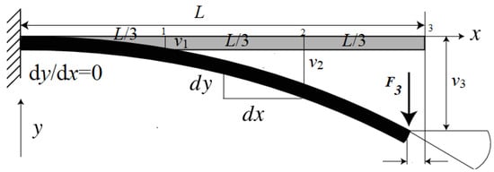
Figure 1.
A cantilever beam represented by three nodes.
To obtain a closed-form solution, the parameter is defined as (see [8])
where is the frequency in rad.s−1. For a cantilever beam, the boundary conditions at the fixed end are:
By assuming n nodes across the beam length, for each node i we assign a kernel collocation function such that, at node i (or at ),
In the RKPM, the transverse displacement is approximated in terms of such that represents the effects of all the nodes according to
From (4) and (5), it is obvious that . Note that in the FEM always. By using Equation (5), the RKPM always incorporates more approximations than the FEM.
If the cantilever beam is divided into three equal lengths of L/3 (see Figure 1), then for any mesh-free method the governing differential equation is assigned to each node individually, giving three equations:
From (5), the approximate displacement is
Each function in (7) is the product of two functions such that
where is called the collocation function, and is the kernel function. Generally, the collocation function is designated by , see [4,5,6,7]. Herein, is used to represent all nodes (globally supportive). Moreover, is chosen so that the approximate displacement in (7) always satisfies the boundary conditions in (3), i.e.,
The collocation and kernel parts are therefore defined according to (10), giving the kernel collocation function defined in (11). In Equations (10) and (11), the coefficients A, B and C depend on the location of the nodes and are determined later.
3. Parametric Study
Nine kernel collocation function values are required to define Equation (7) at three nodes:
Substituting from Equation (11) in Equation (12) gives
The node locations are:
Substitution of into the differential Equation (6) requires the fourth derivative of to be calculated. Considering (8), this derivative is
The transverse displacement of each oscillating node can be written as
Substitution of Equation (14) into (9), while satisfying Equation (4) yields
where A, B and C are the coefficients of the collocation function.
Equation (17) can be solved symbolically [9] to give the coefficients of the collocation function in terms of L as,
By substituting Equation (18) into (13) we have , which can be substituted into Equations (7) and (15). Thereafter, Equations (7) and (15) can be combined with Equations (6) and (16) and after a lengthy algebraic manipulation, we have
From Equation (13), the elements of the matrix, in (19), are functions of the kernel-adjusting parameter k, which is embedded in the following nine equations:
The matrix elements are simple numeric values that have been calculated by varying k using an automatic symbolic operation [9]. It was found that when , the system of Equation (19) reduces to:
From Equation (21), which is a simple eigenvalue problem, the fundamental frequency for free vibration of the cantilever determined according to the RKPM can be defined in terms of the beam parameters from
Note that only three nodes have been used to derive (22).
The closed form solution for the exact fundamental frequency of a cantilever is derived in [8] by finding the first root of the following transcendental equation,
where is related to the exact fundamental frequency by
The first root of Equation (23) is
giving the exact fundamental frequency
Comparing (22) and (26),
This illustrates that the kernel function parameter k can be adjusted to achieve an exact solution. However, for the value of k in Equation (27) the second natural frequency is not the same as the analytical result (see Table 1). This raises the question of whether the FEM approach can lead to an accurate result for the second natural frequency. As far as the author is aware, there is no answer to this question in the open literature. This is investigated below using a procedure similar to that leading to Equation (19).

Table 1.
Natural frequencies predicted by mesh-free and FE methods.
It should be remembered that an inappropriate Kernel parameter leads to substantial errors, as indicated in Figure 2. Therefore, when a straightforward route for a Kernel adjustment does not exist, using a Kernel collocation mesh-free method cannot be recommended. However, this paper does not discuss the Kernel adjustment routes and compares with the FEM only.
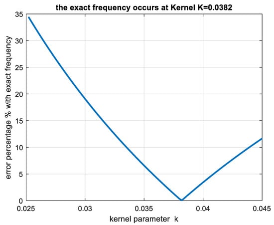
Figure 2.
Error percentage versus Kernel parameter.
4. Parametric Study of the Finite Element Solution
Vibration analysis by the FEM is well established. The method described in [10] is used to obtain a solution. Only three elements are used (Figure 1) to obtain a direct comparison with the mesh-free method. The stiffness matrix of an element in bending is given in [10] as,
In Equation (28), l is the length of each element, the elastic modulus is and the second moment of area is . The mass matrix is also given in [10] as,
where is the cross cross-sectional area and is the density. By substituting the element length of l = L/3 in Equations (28) and (29), applying an assembling procedure and implementing the boundary conditions, the overall stiffness matrix is
Since the displacement and slope of the clamped end is zero, the stiffness matrix reduces to a 6 × 6 matrix in Equation (30). Similarly, the overall mass matrix is 6 × 6:
Relating the mass and stiffness matrices through the well-known equation, similar to Equation (19):
where the vector expresses the displacements and slopes of three nodes as
The natural frequencies of the system can then be determined from
Again, by using the symbolic manipulation tool [9], the roots of the Equation (34) can be computed in terms of the beam parameters. The first and second natural frequencies predicted by the three-element FE model are displayed in the last row of Table 1. The natural frequencies predicted using one and two elements are also shown in Table 1. Using three elements provides better results than using two elements. However, by using three elements, we obtain six natural frequencies, and we have mentioned only the first two in Table 1. The other four modal frequencies represent higher modes. In FEM studies, sometimes the higher modes should be ignored for the sake of accuracy. A technique known as Component Mode Synthesis (CMS) [11] may help to recognise and eliminate the undesired modes.
The information in Table 1 indicates that the error 2nd Natural frequency does not follow a regular pattern in the FEM, i.e., by increasing the number of elements from two to three the error is grown from 3.8% to 6.9%. In fact, the erroneous behaviour of the FEM in higher modes is a disadvantage that is well known in vibration analysis. Similar disadvantages exist in the Kernel collocation (mesh-free) method if a clear and transparent method for the Kernel adjustment method is not available.
5. FRF Determination
The frequency response function (FRF) is a term related to forced vibration studies (see [8]). Herein, the FRF relates the tip deflection to a transverse force applied at the tip, where
The acceleration at the tip can, therefore, be described by
In Equation (36), the parameter and indicates the fraction of the total beam mass m that acts at the cantilever tip and is the elastic resistance force at the tip. Therefore, the third equation in (6) (i.e., at the third node) needs to be modified to the following form:
In (37), is the delta function, so multiplying the term by defines the loading as a concentrated force at the tip. By substituting (36) and (16) into the first and second equations in (6) and (37) and by incorporating Equations (24)–(26), after substantial manipulation, the result is:
The FRF is a deflection per unit force. In order to determine this FRF, it is first necessary to define a frequency-dependent matrix, designated by , as
The FRF is then determined in dimensionless form from Equations (38) and (39). Defining , then the FRF would be:
The closed-form solution for the tip FRF of a cantilever is given in [8] as
which, in dimensionless form, gives
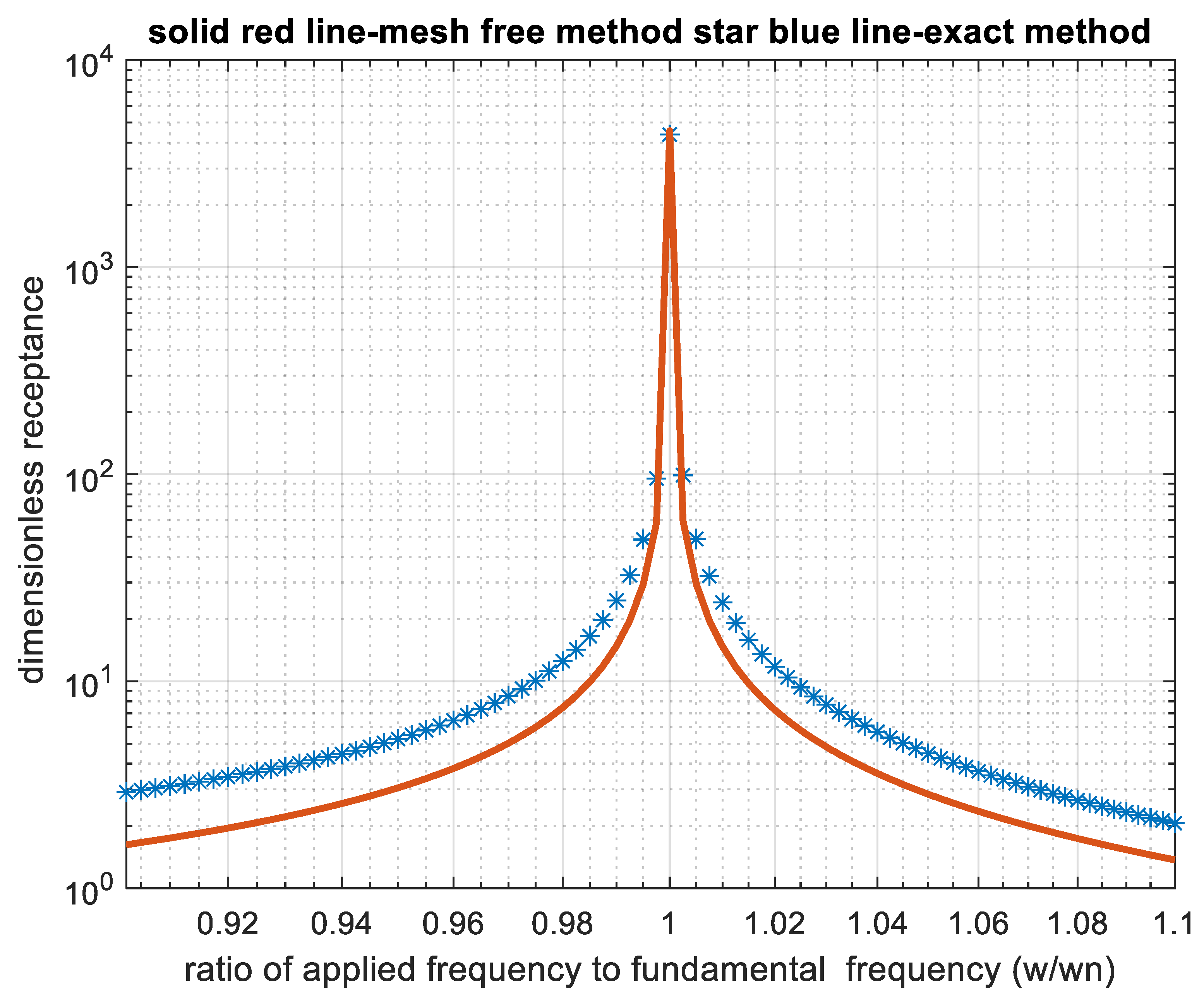
In Equation (42), is related to via Equation (2). The exact and approximate (for and ) FRF functions are plotted in Figure 3 as a function of dimensionless frequency. As discussed earlier, both plots show a resonance peak at the same frequency. Moreover, the magnitude of this peak, resulting from both the approximate and exact solutions, is also the same. Clearly, by choosing an appropriate mass fraction and kernel parameter k, the results have been the same with exact solutions only in the pick where the natural frequency in both methods is the same. Therefore, mesh-free methods could be used to analyse both the forced vibration and the free vibration and provide accurate results.

Figure 3.
Comparing dimensionless FRF at tip (mesh-free with exact).
According to Figure 3, it is impossible to find an identical FRF for the exact, mesh-free and FEM. Herein, we compare the theoretical FRF only, and the experimental FRF that depends on damping, material heterogeneity, etc., is not in the scope of this paper. It is obvious that the FRF peaks coincide only when we use an adjusted Kernel and .
6. Aim and Motivation
The aim of this article is to compare the mesh-free method with the finite element method (FEM) when applied to a specific problem for which an analytical solution is available. This allows for the determination of the error in each method. This research fills a gap, as no prior studies have directly compared mesh-free methods to the FEM in the context of vibration analysis or similar problems in the literature.
Without such comparisons, researchers acknowledge that some mesh-free methods can achieve high accuracy through kernel adjustments, as demonstrated in this paper. Consequently, efforts have been made to combine mesh-free methods with the FEM to enhance accuracy [12]. Likewise, the FEM can be adjusted through changes in mesh size or shape function types, but in some cases, this still does not yield sufficient accuracy. For instance, hybrid methods like the “Free Element Collocation Method” [13] have been developed to combine the advantages of both mesh-free and FEM approaches.
In mesh-free methods, nodes are used without the need for elements, but recent developments have introduced methods that are purely mesh-free, such as Deep Neural Networks (DNNs), which solve partial differential equations (PDEs) [14]. While DNN-based methods have been compared with the FEM, they represent a distinct approach. The contribution of this article, therefore, has not been previously addressed in the literature.
The comparison in this paper is limited to 1D forced and free vibration analysis of the beams. Therefore, the conclusions cannot be general except for the effect of Kernel adjustment on accuracy that is demonstrated and is applicable in general.
7. Conclusions
In this article, by considering a benchmark problem, a new mesh-free method is used for the analysis of flexural vibrations. The parametric investigation enabled the exactness of the method to be evaluated and compared with the accuracy of the FEM. It was shown that adjustment of two parameters can provide an identical solution to an exact closed-form solution. However, by increasing the number of elements in the FEM, the modal frequencies approach the exact result. These increased elements cause extra undesired modal frequencies, which should be ignored for the sake of accuracy. Finally, to answer the question of applicability, it can be concluded that the mesh-free method is not advantageous if the kernel adjustment is not available, but the finite element also suffers from extra numbers of modal frequencies. If it could be cured by CMS [11], it would be advantageous. Although this conclusion is limited to flexural vibration only, the effect of Kernel adjustment on accuracy seems to be a general one and mathematically demonstrated in this paper.
Funding
This research received no external funding.
Data Availability Statement
The data presented in this study are available in the article.
Conflicts of Interest
The author declares no conflict of interest.
References
- Tanaka, S.; Ejima, S.; Wang, H.; Sadamoto, S. Free vibration analysis of thin-walled folded structures employing Galerkin-based RKPM and stabilized nodal integration methods. Eng. Anal. Bound. Elem. 2024, 163, 308–317. [Google Scholar]
- Ghamsari Esfahani, S.; Sarrami-Foroushani, S.; Azhari, M. On the use of reproducing kernel particle finite strip method in the static, stability and free vibration analysis of FG plates with different boundary conditions and diverse internal supports. Appl. Math. Model. 2021, 92, 380–409. [Google Scholar]
- Qi, D.; Wang, D.; Deng, L.; Xu, X.; Wu, C.T. Reproducing kernel mesh-free collocation analysis of structural vibrations. Eng. Comput. 2019, 36, 734–764. [Google Scholar] [CrossRef]
- Li, S.; Liu, W.K. Mesh-free and particle methods and their applications. ASME Appl. Mech. Rev. 2002, 54, 1–34. [Google Scholar] [CrossRef]
- Liu, W.K.; Jun, S.; Li, S.; Adee, J.; Belytschko, T. Reproducing Kernel Particle Methods for Structural Dynamics. Int. J. Numer. Methods Eng. 1995, 38, 1655–1679. [Google Scholar] [CrossRef]
- Zhou, J.; Zhang, H.; Zhang, L. Reproducing kernel particle method for free and forced vibration analysis. J. Sound Vib. 2005, 279, 389–402. [Google Scholar]
- Shaw, A.; Roy, D.; Reid, S.R.; Aleyaasin, M. Reproducing kernel collocation method applied to the non-linear dynamics of pipe whip in a plane. Int. J. Impact Eng. 2007, 34, 1637–1654. [Google Scholar]
- Bishop, R.E.D.; Johnson, D.C. The Mechanics of Vibration; Cambridge University Press: Cambridge, UK, 1960. [Google Scholar]
- Moler, C.; Costa, P.J. Symbolic Math Toolbox with MATLAB; Math Works, Inc.: Natick, MA, USA, 1997. [Google Scholar]
- Petyt, M. Introduction to Finite Element Vibration Analysis; Cambridge University Press: Cambridge, UK, 1990. [Google Scholar]
- Masson, G.; Brik, B.A.; Cogan, S.; Bouhaddi, N. Component mode synthesis (CMS) based on an enriched ritz approach for efficient structural optimization. J. Sound Vib. 2006, 296, 845–860. [Google Scholar]
- Huerta, A.; Fernández-Méndez, S.; Liu, W.K. A comparison of two formulations to blend finite elements and mesh-free methods. Comput. Methods Appl. Mech. Eng. 2004, 193, 1105–1117. [Google Scholar]
- Gao, X.W.; Gao, L.F.; Zhang, Y.; Cui, M.; Lv, J. Free element collocation method—A new method combining advantages of finite element and mesh free methods. Comput. Struct. 2019, 215, 10–26. [Google Scholar]
- Zhu, X.; He, M.; Sun, P. Comparative Studies on Mesh-Free Deep Neural Network Approach versus Finite Element Method for Solving Nonlinear Hyperbolic Wave Equations. Int. J. Numer. Anal. Model. 2022, 19, 603–629. [Google Scholar]
Disclaimer/Publisher’s Note: The statements, opinions and data contained in all publications are solely those of the individual author(s) and contributor(s) and not of MDPI and/or the editor(s). MDPI and/or the editor(s) disclaim responsibility for any injury to people or property resulting from any ideas, methods, instructions or products referred to in the content. |
© 2025 by the author. Licensee MDPI, Basel, Switzerland. This article is an open access article distributed under the terms and conditions of the Creative Commons Attribution (CC BY) license (https://creativecommons.org/licenses/by/4.0/).