Identification of Parkinson’s Disease from Native Italian People: Machine Learning Voice Analysis

Abstract

Background: Parkinson’s Disease (PD) is a neurodegenerative disorder frequently accompanied by speech impairments, which could serve as non-invasive biomarkers for early detection. This study investigates the efficacy of machine learning models trained on voice and speech acoustic features for distinguishing PD patients from healthy controls (HC) using the publicly available Italian Parkinson’s Voice and Speech (IPVS) dataset. Methods: A comprehensive set of acoustic features was extracted, including perturbation, prosodic and temporal features, Mel-Frequency Cepstral Coefficients (MFCCs), and Gammatone Cepstral Coefficients (GTCCs). These features were evaluated individually and in combination using six supervised classifiers: Support Vector Machine (SVM), Decision Tree (DT), Random Forest (RF), K-Nearest Neighbors (KNN), XGBoost (XGB), and Multi-Layer Perceptron (MLP). Results: The best-performing configuration combination of GTCC and acoustic features with the SVM model achieved 94.68% accuracy, 94.37% sensitivity, 95.04% specificity, 95.71% precision, 96.04% F1-score, an MCC value of 0.89, and an ROC-AUC of 0.98. In the combination of all feature sets, the most impressive performance was observed with the MLP classifier. This achieved 93.08% test accuracy, 94.30% sensitivity, 91.18% specificity, 94.30% precision, 94.30 F1-score, an ROC-AUC of 0.97, and an MCC value of 0.85. Conclusions: The findings demonstrate that combining clinically relevant acoustic features with robust machine learning classifiers offers a reliable, interpretable, and computationally efficient solution for PD detection. The use of a publicly available dataset, open-source tools, and subject-wise validation contributes to the reproducibility and clinical relevance of the proposed approach. This study reinforces the potential of speech as a digital biomarker for early PD detection and supports the integration of voice-based assessments into diagnostic platforms.

1. Introduction

There are several neurodegenerative disorders affecting the nervous system, including Parkinson’s disease (PD), which mainly results from the degeneration of dopaminergic neurons of the substantia nigra [1]. It leads to motor symptoms such as tremors, rigidity, postural instability and bradykinesia [2,3]. PD is largely caused by a complex interaction between genetic predisposition and environmental exposure. Among different categories of workers, seafarers face a higher risk of developing Parkinson’s disease due to prolonged occupational exposure to neurotoxic chemicals, such as solvents, exhaust fumes, and pesticides found in the maritime environment. This risk is compounded by the physical demands, high-stress conditions, and irregular sleep schedules inherent to seafaring life. PD is also highly associated with speech and voice impairments, collectively known as hypokinetic dysarthria [4,5]. Up to 90% of people with PD have voice deficits manifesting as reduced pitch variation, monophasic intonation, breathy or hoarse voice quality, and articulatory imprecision [5,6,7]. Speech abnormalities have become increasingly recognized as promising non-invasive biomarkers of PD because of their early onset and high incidence [8,9].

PD is diagnosed by experienced specialists based on clinical evaluation, neurological examination, and dopaminergic medication response [10]. This type of assessment is subjective, costly, and may not be able to provide a timely diagnosis, especially in resource-limited contexts [10,11]. As an alternative, automated speech analysis can be used to detect and monitor PD in a more scalable, cost-effective, and objective manner. Recent advancements in digital signal processing as well as machine learning (ML) have enabled the extraction and classification of subtle acoustic anomalies from speech recordings, allowing for remote screening and digital phenotyping of neurological disorders [12].

Research has explored the acoustic features of speech to characterize PD-related speech alterations [13]. These include perturbation-based measures such as jitter and shimmer; prosodic features such as pitch and intensity; noise metrics such as the harmonic-to-noise ratio (HNR); and spectral features such as Mel-Frequency Cepstral Coefficients (MFCCs) and Gammatone Cepstral Coefficients (GTCCs) [14,15]. These features capture phonatory instability, spectral distribution, and articulatory dynamics affected in PD. In addition, deep learning approaches based on time-frequency representations such as spectrograms and short-time Fourier transforms (STFT) have demonstrated strong performance in PD classification tasks [16,17,18]. Several existing studies employ heterogeneous datasets, different preprocessing pipelines, and varying validation strategies, making direct comparison difficult [19,20]. Furthermore, while MFCCs are widely used in PD speech analysis, the utility of GTCCs remains comparatively underexplored, particularly within the native Italian speech dataset. There is also limited evidence regarding the extent to which GTCC features complement traditional acoustic descriptors and whether feature fusion consistently improves classification performance across different machine learning models.

This study has used the Italian Parkinson’s Voice and Speech dataset [21,22,23], a publicly available and noise-controlled corpus collected from native Italian speakers under standardized conditions. The dataset comprises multiple speech tasks designed to capture phonatory, articulatory, and prosodic characteristics relevant to PD. In this work, we have extracted a diverse set of handcrafted acoustic features, including perturbation, prosodic and temporal features, MFCC, and GTCC descriptors, and evaluated their performance across six widely used machine learning (ML) algorithms: Support Vector Machine (SVM), Decision Tree (DT), Random Forest (RF), K-Nearest Neighbors (KNN), XGBoost (XGB), and Multi-Layer Perceptron (MLP).

This work aims to provide a systematic comparative benchmark of different speech feature representations for PD detection within a consistent experimental framework. The study is guided by the following research questions: (a) How do acoustic, MFCC, and GTCC feature representations compare in their ability to distinguish PD speech from healthy controls within the IPVS dataset? (b) Does feature fusion improve classification performance compared with individual feature representations? (c) Which traditional machine learning classifier provides the most robust performance across the evaluated feature sets?

The primary contribution of this work is a comprehensive comparison of acoustic, MFCC, GTCC, and fused feature representations using multiple traditional machine learning algorithms under a reproducible and subject-independent evaluation framework. The findings provide insight into the relative effectiveness of these feature representations and establish a benchmark for future investigations of speech-based digital biomarkers for Parkinson’s disease.

2. Materials and Methods

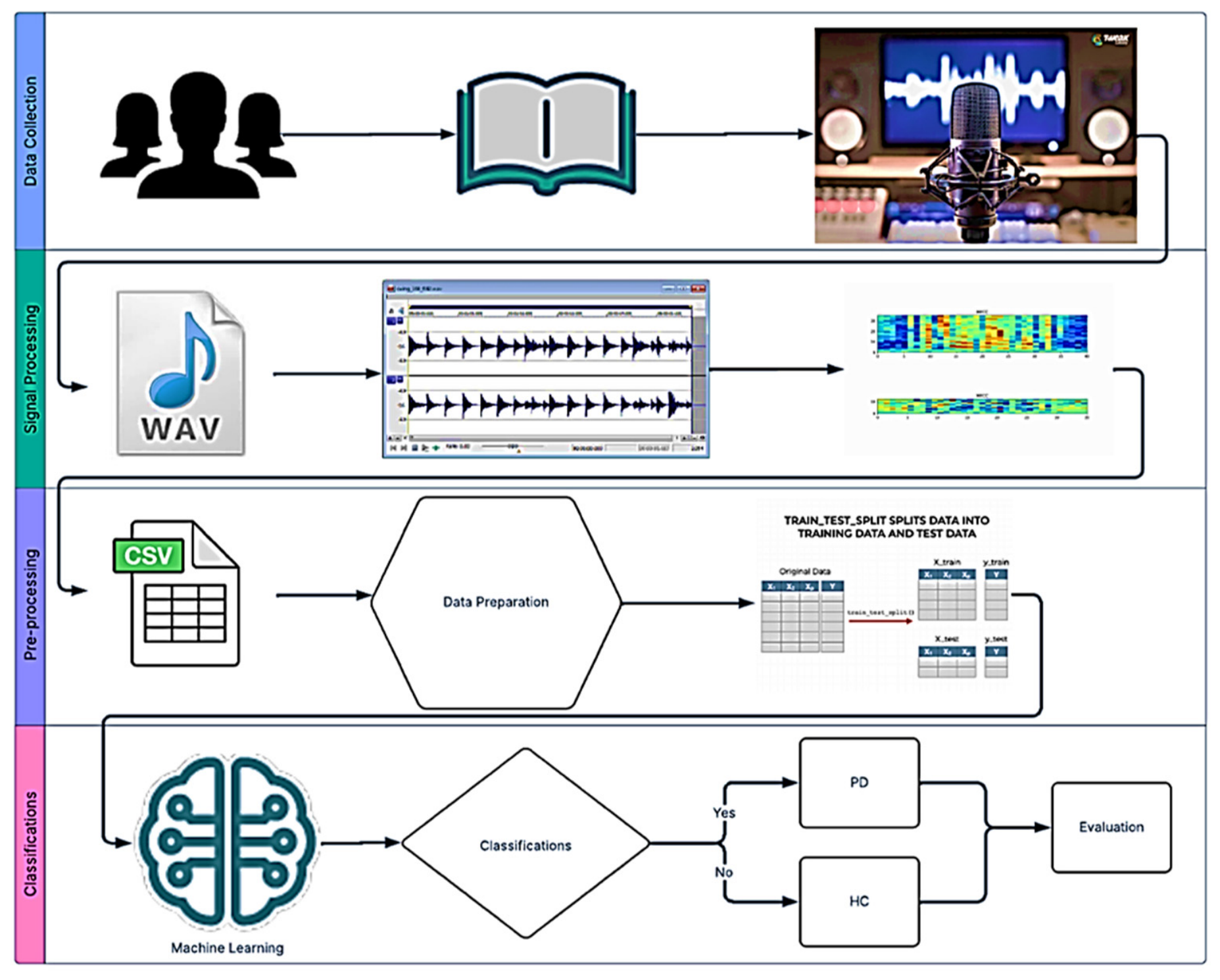
Figure 1 illustrates the overall workflow of the study. It includes data collection, signal processing, data preprocessing, and the development and evaluation of ML models for PD classification. The process was carried out using Python 3.

At the data collection stage, speech recordings from the IPVS dataset were downloaded from the authors’ provided online server [23]. The signal processing stage involved extracting relevant acoustic and spectral representations, Cepstral coefficients, and other clinically relevant voice features.

The data preprocessing stage included normalization, noise reduction, and segmentation to enhance feature quality and ensure comparability across samples. Finally, at the model development and evaluation stage, multiple supervised ML algorithms were implemented and carefully assessed using a subject-independent cross-validation approach to minimize data leakage and ensure robust performance estimation. The detailed procedures for each stage are described in the following subsections.

2.1. Data Collection

Participants: This study utilized the publicly available IPVS dataset [23], comprising voice recordings collected from native Italian speakers, mostly living in the Bari region. The data collection was planned and coordinated by Di Mario and is available under the Creative Commons Attribution License (CC BY 4.0). Detailed information regarding participant inclusion/exclusion criteria and recording protocols is provided in Di Mario et al. [21,22].

The dataset includes 65 participants, stratified into three subgroups:

• Young Healthy Controls (YHC): 15 individuals aged 19–29 years (13 males, 2 females), with no reported speech or language impairments.
• Elderly Healthy Controls (EHC): 22 individuals aged 60–77 years (10 males, 12 females), also free from speech or language disorders.
• Parkinson’s Disease (PD) patients: 28 individuals (19 males, 9 females), aged 40–80 years, all undergoing antiparkinsonian treatment. Disease severity was assessed using the Hoehn and Yahr (H&Y) scale, with most patients classified as stage <4. One participant was classified as stage 5 and two as stage 4. Unified Parkinson’s Disease Rating Scale motor subsection (UPDRS-III) scores ranged from 1 to 24, with 10 patients scoring 1–10 and 18 patients scoring 11–24.

Voice Recording Protocol

The voice audio signals were collected using a standardized protocol developed in collaboration with neurologists, speech therapists, and clinicians to ensure clinical relevance and consistency. Participants performed vocal tasks, including:

(a) Reading two phonemically balanced Italian texts to assess prosody and articulation.

(b) Rapid repetition of the syllables “pa” and “ta” to evaluate motor agility.

(c) Sustained phonation of the vowels/a/, /e/, /i/, /o/, /u/ reviewed to evaluate voice quality, respiratory support, and phonatory stability, with both maximum phonation duration and fixed 5 s intervals, and

(d) Reading of phonemically balanced words and phrases to probe articulation in varied phonetic contexts.

Pauses between tasks were standardized to allow recovery and consistent effort. This multi-faceted recording protocol captures a broad range of speech and voice characteristics, enabling the extraction of both acoustic and temporal features for the quantitative analysis of speech intelligibility, motor control, and potential markers of neurodegenerative disease progression. Voice was recorded in optimal condition with professional microphones and stored in .wav file format. Further procedural details can be found in the primary dataset publication [21,22].

2.2. Signal Preprocessing

The dataset contained 831 audio recordings. There are 349 voice recordings from EHC, 45 recordings from YHC and 437 voice files (.wav) from PD participants. The recordings were collected at multiple sampling rates. In the initial step, all audio recordings were preprocessed to ensure consistency and minimize recording artifacts. First, each signal was resampled at a fixed sampling rate of 16 kHz to standardize temporal resolution across the dataset. To reduce background noise and enhance speech clarity, a spectral noise reduction algorithm was applied using the open source “noisereduce 3.0.3” Python library by Tim Sainburg [24,25]. This library implements adaptive spectral gate techniques inspired by classical noise suppression methods. Following noise reduction, amplitude normalization was performed by scaling each audio waveform to the range [−1, +1] based on its peak absolute amplitude. This normalization step reduces the potential impact of variations in speaker-to-microphone distance and recording conditions on subsequent feature extraction and classification stages. The entire preprocessing pipeline, including resampling, noise reduction, and normalization, was implemented and automated in Python3. This was to ensure reproducibility and consistent application across all recordings.

Feature Extraction

A comprehensive set of acoustic features was extracted to capture vocal biomarkers associated with Parkinson’s speech. All healthy controls, including both Young HC and Adult HC recordings, were merged into a single HC class prior to model training. The study explicitly states that only acoustic, MFCC, and GTCC features extracted from audio signals were used as input to the machine learning models, and no demographic attributes such as age, gender, or clinical metadata were incorporated into the feature space. All signals were first resampled at a standard sampling rate of 16 kHz. They were preprocessed through amplitude normalization and denoised to minimize variability due to recording conditions and background noise. Perturbation features were computed using two widely used softwires for phonetic and acoustic signal analysis Parselmouth (Praat-6.4.65 python interface), introduced by Yannick Jadoul et al. [26], and PyDub, a Python library developed by James Robert [27]. The jitter parameters included local jitter, absolute jitter, RAP, PPQ5, and DDP, while the shimmer parameters included local shimmer, shimmer in dB, APQ3, APQ5, and DDA. These were summarized using statistical functions: mean, standard deviation, and range.

Prosodic Features: Fundamental frequency (F0) was extracted using an autocorrelation-based pitch detection algorithm, yielding minimum, maximum, and mean pitch values. Intensity-based features (mean, min, max) are also derived. The Harmonic-to-Noise Ratio (HNR) was computed to evaluate vocal periodicity.

Temporal Features: Total pause duration and speech-to-total duration ratio were computed via energy-based silence detection, offering insight into articulatory timing and fluency.

Spectral Features: Mel-Frequency Cepstral Coefficients (MFCCs) and Gammatone Cepstral Coefficients (GTCCs) were extracted using the librosa 0.11.0 library. Each 13-dimensional coefficient vector was summarized using statistical functionals to yield fixed-length feature vectors.

2.3. Data Preprocessing and Partitioning

Extracted features from the raw audio signal were saved into three CSV files: one for acoustic features, and one each for MFCCs and GTCCs. The dataset files were imported into a Jupyter Notebook 7.5 environment using the Pandas 3.0.1 library for further processing and analysis. Initial steps included exploration data analysis involving graphical visualization and statistical summaries. Subsequently, the dataset was screened for missing values and duplicate entries, which were removed to ensure data integrity. The classification target was defined by the “label” column, where a value of 1 indicated a PD case and 0 indicated HC.

To prevent data leakage and overoptimistic performance estimates, a subject-wise split strategy was implemented. Because signal processing generated multiple audio-derived feature files per participant, traditional random splitting would risk distributing a single individual’s data across both training and testing subsets. To avoid this, all samples belonging to a participant were grouped using unique subject identifiers and treated as a single unit during partitioning. The subjects were randomly shuffled while maintaining class representation and divided into training (75%) and testing (25%) subsets. Post-split verification confirmed that no participant appeared in both subsets.

No resampling techniques, such as oversampling or undersampling, were applied. The original class distribution was retained to preserve the natural characteristics of the dataset and reflect realistic clinical conditions.

Feature standardization was performed using the StandardScaler function from the scikit-learn library, which transforms each feature to have zero mean and unit variance. Standardization was fitted exclusively on the training data and subsequently applied to the corresponding validation and test data to prevent information leakage.

Experiments Setup

We conducted three separate experiments to evaluate the effectiveness of these features in distinguishing between PD and HC.

Experiment 1: Individual feature evaluation, where acoustic features, MFCCs, and GTCCs were assessed independently.

Experiment 2: Pairwise feature fusion, where combinations of two feature groups (Acoustic with MFCC, Acoustic with GTCC, and MFCC-GTCC) were evaluated.

Experiment 3: All the features were combined to assess their collective discriminative power. Each experiment was assessed using multiple machine learning classifiers.

2.4. ML Model Development and Evaluation

Six supervised ML algorithms: Support Vector Machine (SVM), Extreme Gradient Boosting (XGB), Random Forest (RF), Decision Tree (DT), K-Nearest Neighbors (KNN), and Multi-layer Perceptron (MLP) were implemented for the binary classification of PD and HC participants. To ensure a fair comparison among classifiers and identify optimal model configurations, hyperparameter optimization was performed using the GridSearchCV framework available in the scikit-learn library.

GridSearchCV conducts an exhaustive search across predefined hyperparameter combinations using 10-fold cross-validation on the training set. For each configuration, the training data was partitioned into 10-folds, with nine folds used for training and one fold used for validation. This procedure was repeated until each fold had served as the validation set once. The average cross-validation performance across all folds was then used to rank candidate hyperparameter combinations, and the configuration yielding the best average score was selected.

Hyperparameter optimization was performed exclusively on the training set. No data from the independent test set was used during model selection, parameter tuning, or preprocessing parameter estimation. After identifying the optimal hyperparameters, each classifier was retrained using the complete training set and subsequently evaluated on the independent subject-wise test set. The complete list of classifiers and optimized hyperparameter search spaces is provided in

Table 1. Models and Parameters.

Algorithm Name	Parameters
Support Vector Machine (SVM)	C = 10, gamma = ‘auto’, probability = True
Decision Tree (DT)	max_depth = 10, max_features = ‘sqrt’, min_samples_split = 5, random_state = 42
Random Forest (RF)	n_estimators = 200, random_state = 42
K-Nearest Neighbors (KNN)	metric = ‘manhattan’, n_neighbors = 7
XGBoost Classifier	colsample_bytree = 1.0, eval_metric = ‘mlogloss’, learning_rate = 0.1, n_estimators = 100, random_state = 42
Multilayer Perceptron (MLP)	Alpha = 0.001, hidden_layer_sizes = (50,), max_iter = 300, random_state = 42

.

3. Results

After determining the optimal hyperparameters, each classifier was retrained using the entire training set and subsequently evaluated on the independent subject-wise test set. Performance was assessed using Accuracy, Precision, Recall, F1-score, Receiver Operating Characteristic Area Under the Curve (ROC-AUC), and Matthews Correlation Coefficient (MCC). All reported results correspond to this final evaluation on previously unseen subjects. Across the three experimental configurations, six classifiers were trained and evaluated using different combinations of acoustic and spectral feature sets.

3.1. Performance Metrics

To assess model performance, we employed a range of metrics derived from the confusion matrix. There are four possible outcomes for each output of a binary classifier, which are outlined as follows.

Confusion Matrix: In

Table 2. Confusion matrix.

	Actual Positive	Actual Negative
Predicted Positive	True Positive (TP): Correctly classified PD	False Positive (FP): HC misclassified as PD
Predicted Negative	False Negative (FN): PD misclassified as HC	True Negative (TN): Correctly classified HC

, each column shows all real positive (TP + FN) and real negative (FP + TN), while each row shows all predicted positive (TP + FP) and predicted negative (FN + TN). The true and false positives and negatives are used to calculate several metrics that are useful for model evaluation. This study considers seven evaluation criteria.

Accuracy: the portion of classifications that were correct, whether negative or positive.

$$Accuracy={\displaystyle \frac{correct classifications}{total classifications}}={\displaystyle \frac{TP+TN}{TP+TN+FP+FN}}$$

Recall or Sensitivity: The true positive rate (TPR), the proportion of all actual positives that were correctly identified.

$$Recall or\left(TPR\right)={\displaystyle \frac{correctly classified actual positive}{all actual postives}}={\displaystyle \frac{TP}{TP+FN}}$$

Specificity: Also known as true negative rates, these indicate actual negative cases that the model accurately identified as negative

$$Specificity={\displaystyle \frac{correctly cllassified actual Negative}{everything classified as Negative}}={\displaystyle \frac{TN}{TN+FP}}$$

Precision: The proportion of positive predictions that were actually correct.

$$Precision={\displaystyle \frac{correctly cllassified actual postive}{everything classified as positive}}={\displaystyle \frac{TP}{TP+FP}}$$

The F1-score is the harmonic mean of precision and recall.

$$F1-Score=2\times {\displaystyle \frac{Precision\times Reacll }{Precision+Recall}}$$

Matthew’s correlation coefficient (MCC): Measures the quality of a classifier; it summarizes all elements of the confusion matrix into a single metric.

$$MCC={\displaystyle \frac{TP\times TN-FP\times FN}{\sqrt{\left(TP+FP\right)\left(TP+FN\right)\left(TN+FP\right)(TN+FN)}}}$$

Receiver-operating characteristic curve (ROC): The ROC curve is the visual representation of model performance, formed by plotting the true positive rate (TPR) against the false positive rate (FPR). An ideal classifier reaches TPR 1 and FPR 0.

Area under the curve (AUC): Measures a classifier’s ability to distinguish between the two classes. An AUC of 1.0 denotes perfect separability, while an AUC of 0.5 denotes pure guessing.

3.2. Experiment 1: Individual Feature Subgroup Evaluation

In this experiment, each feature group, Acoustics, MFCCs, and GTCCs, was evaluated independently across six classifiers.

Table 3. ML models’ performance score on individual features.

Features	Model	Train ACC	Test ACC	Sen	Spe	Pre	F1	ROC-AUC	MCC
Acoustics	SVM	92.42	87.88	89.62	85.87	87.96	88.79	0.94	0.75
	XGB	99.84	83.33	87.74	78.26	82.30	84.93	0.93	0.66
	RF	99.68	80.30	84.91	75.00	79.65	82.19	0.89	0.60
	DT	99.68	67.68	69.81	65.22	69.81	69.81	0.72	0.35
	KNN	100	82.83	82.08	83.70	85.29	83.65	0.88	0.65
	MLP	88.47	83.84	86.79	80.43	83.64	85.19	0.92	0.67
MFCCs	SVM	92.58	84.26	83.21	86.67	93.44	88.03	0.90	0.66
	XGB	100	73.76	81.02	90.00	94.87	87.40	0.93	0.66
	RF	100	83.76	81.02	90.00	94.87	87.40	0.89	0.66
	DT	94.79	71.57	68.61	78.33	87.85	77.05	0.75	0.43
	KNN	100	80.71	78.83	85.00	92.31	85.04	0.89	0.59
	MLP	80.28	78.68	76.64	83.33	91.30	83.33	0.86	0.56
GTCCs	SVM	98.71	81.04	77.54	87.67	92.24	84.25	0.93	0.62
	XGB	100	80.09	75.36	89.04	92.86	83.20	0.90	0.61
	RF	100	74.41	68.12	86.30	90.38	77.69	0.88	0.52
	DT	100	60.19	58.70	63.01	75.00	65.85	0.61	0.21
	KNN	100	73.93	75.36	71.23	83.20	79.09	0.83	0.45
	MLP	79.35	71.09	73.19	67.12	80.80	76.81	0.81	0.39

Abbreviations: SVM: Support Vector Machine; XGB: Extreme Gradient Boosting; RF: Random Forest; DT: Decision Tree; KNN: K-Nearest Neighbors; MLP: Multi-layer Perceptron; MCC: Matthew’s Correlation Coefficient; ROC-AUC: Area under the receiver operating characteristic curve; MFCCs: Mel-Frequency Cepstral Coefficients; GTCCs: Gammatone Frequency Cepstral Coefficients; ACC: Accuracy; Sen: Sensitivity; Spe: Specificity; Pre: Precision.

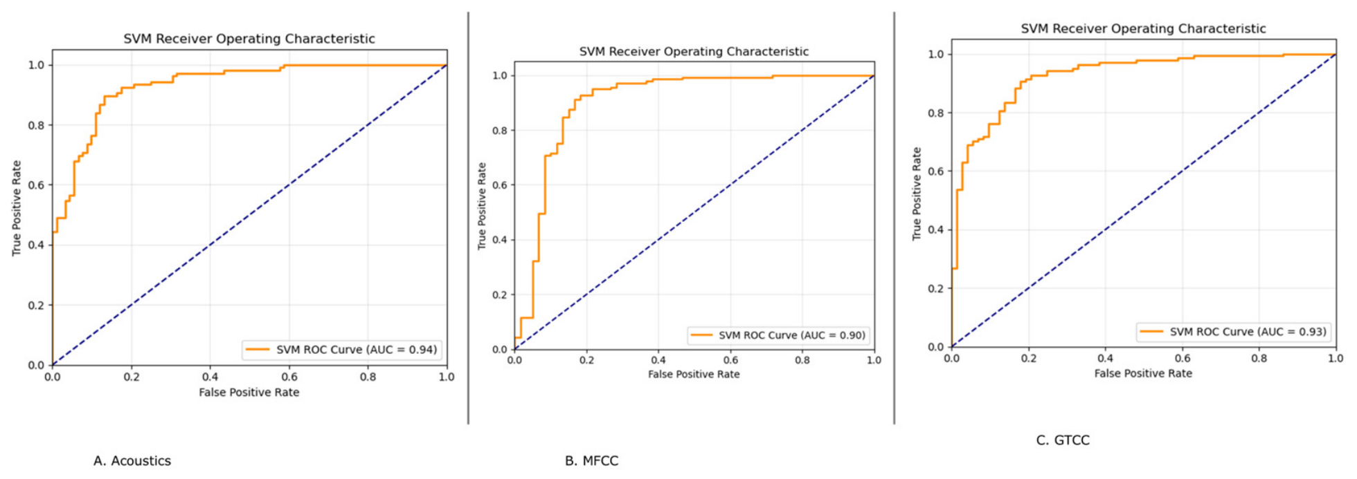
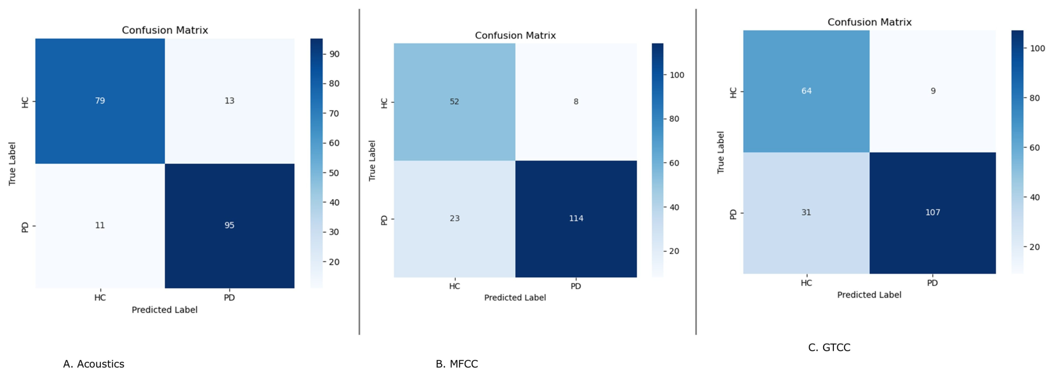
summarizes their scores across the classification performance metrics. All values in the table are shown in percentages except ROC-AUC and MCC. In Figure 2 we show the ROC-AUC and Figure 3 shows the confusion matrix of the best-performing model of each subgroup.

In the first experiment, models were trained and evaluated using individual feature groups: Acoustic, MFCC, and GTCC. Among all models, the SVM model outperformed the other models on each feature group. Acoustic features exhibited the highest performance with a test accuracy of 87.88%, sensitivity of 89.62%, specificity of 85.87%, precision of 87.63%, F1-score of 88.79%, ROC-AUC of 0.94, and an MCC of 0.75. Figure 2A shows the ROC-AUC of the SVM model using the acoustic features group, and Figure 3A represents the confusion matrix.

On the GTCC features, the SVM model achieved an accuracy of 81.04%, sensitivity of 77.54%, specificity of 87.67%, precision of 92.24%, F1-score of 84.25%, ROC-AUC of 0.93, and an MCC of 0.62. Figure 2C indicates the ROC-AUC for the SVM model using GTCC features. In Figure 3C, the confusion matrix is shown.

In the MFCC feature set, the SVM model derived a test accuracy of 84.26%, sensitivity of 83.21%, specificity of 86.67%, precision of 93.44%, F1-score of 88.03%, ROC-AUC of 0.90, and an MCC of 0.66. Figure 2B specifies the ROC-AUC of the SVM model using MFCC features. Figure 3B represents the confusion matrix for the MFCC features and the SVM model.

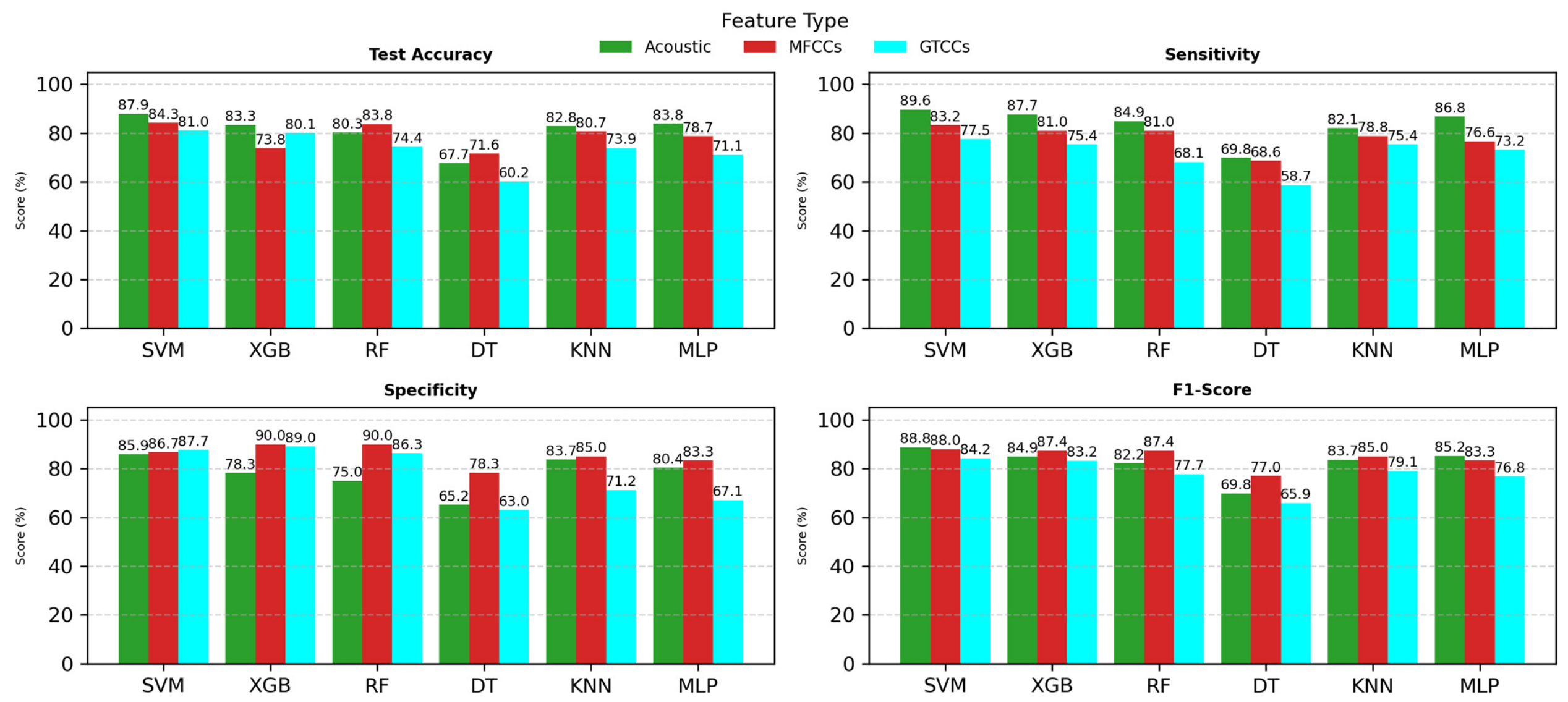
Figure 4 presents a comparative performance analysis of SVM, XGB, RF, DT, KNN, and MLP using three feature sets: acoustic features (green), MFCCs (red), and GTCCs (cyan). The evaluation metrics include test accuracy, sensitivity, specificity, and F1-score, each depicted in separate subplots.

The test accuracy plot is in the top-left; the SVM model achieved the highest accuracy, almost 87.9% across feature types. The sensitivity plot (top-right) shows that the models yielded superior performance with a low-level acoustic-based feature set, particularly SVM (89.6%), XGB (87.7%) and MLP (86.8%), indicating their stronger ability to correctly identify positive cases.

For specificity, the bottom-left plot measures the models’ ability to correctly classify negative cases. XGB and RF exhibited the highest values of up to 90% with MFCC features across most feature types. Meanwhile, the F1-score, shown in the bottom-right results, follows a similar trend, where SVM (88%), RF (87.4%) and XGB (87.4%) models demonstrate the best balance between precision and recall.

Overall, the results highlight that SVM achieved the most stable results, suggesting its strong suitability for voice-based PD detection when combined with cepstral features. These results suggest that low-level acoustic features, when used independently, provide strong discriminatory power for PD detection, particularly when coupled with an SVM classifier.

3.3. Experiment 2: Paired Feature Combinations

In the second experiment, we evaluated the performance of combining two feature subgroups together: (i) Acoustics and MFCC, (ii) Acoustics and GTCC, and (iii) MFCC and GTCC. The performance scores of each model and feature combination are presented in

Table 4. ML models’ performance score on paired feature combinations.

Features	Model	Train ACC	Test ACC	Sen	Spe	Pre	F1	ROC-AUC	MCC
Acoustics + MFCC	SVM	99.83	92.47	89.84	95.50	95.83	92.74	0.97	0.85
	XGB	100	87.45	85.16	90.09	90.83	87.90	0.95	0.75
	RF	100	86.19	84.38	88.29	89.26	86.75	0.94	0.72
	DT	97.64	73.22	72.66	73.87	76.23	74.4	0.74	0.46
	KNN	93.24	84.10	76.69	89.19	89.47	84.30	0.92	0.69
	MLP	90.71	84.10	79.69	89.19	89.47	84.30	0.91	0.69
Acoustics + GTCC	SVM	99.68	94.68	94.37	95.04	95.71	96.04	0.98	0.89
	XGB	100	89.35	90.85	87.60	89.58	90.21	0.96	0.78
	RF	100	88.97	88.73	89.26	90.65	89.68	0.96	0.78
	DT	100	76.96	81.11	74.02	68.87	74.49	0.78	0.54
	KNN	88.38	79.09	76.06	82.64	83.72	79.70	0.89	0.59
	MLP	94.37	93.54	92.96	94.21	94.96	93.95	0.97	0.87
MFCC + GTCC	SVM	99.36	90.64	93.68	87.96	87.25	90.36	0.97	0.81
	XGB	100	89.66	90.53	88.89	87.76	89.12	0.95	0.79
	RF	100	86.70	93.68	80.56	80.91	86.83	0.93	0.74
	DT	97.77	73.89	78.95	69.44	69.44	73.89	0.79	0.48
	KNN	90.13	77.83	84.21	72.22	72.73	78.05	0.88	0.57
	MLP	91.40	84.73	95.79	75.00	77.12	85.45	0.93	0.72

Abbreviations: SVM: Support Vector Machine; XGB: Extreme Gradient Boosting; RF: Random Forest; DT: Decision Tree; KNN: K-Nearest Neighbors; MLP: Multi-layer Perceptron; MCC: Matthew’s Correlation Coefficient; ROC-AUC: Area under the receiver operating characteristic curve; MFCCs: Mel-Frequency Cepstral Coefficients; GTCCs: Gammatone Frequency Cepstral Coefficients; ACC: Accuracy; Sen: Sensitivity; Spe: Specificity; Pre: Precision.

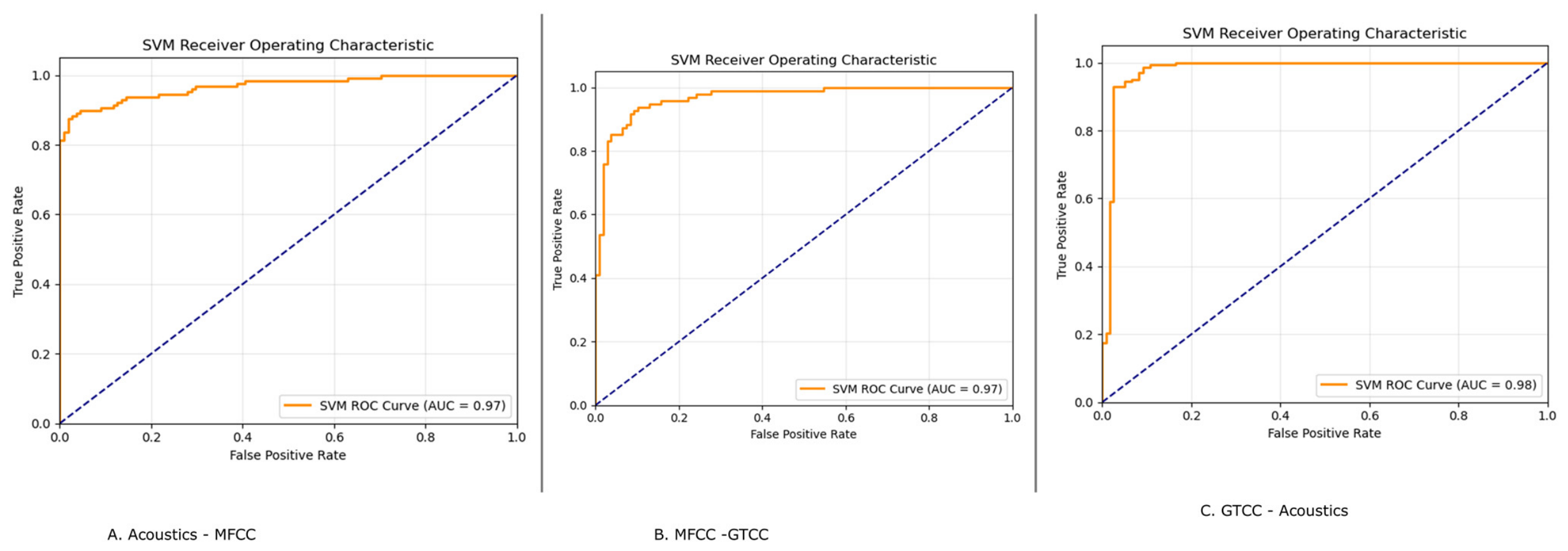
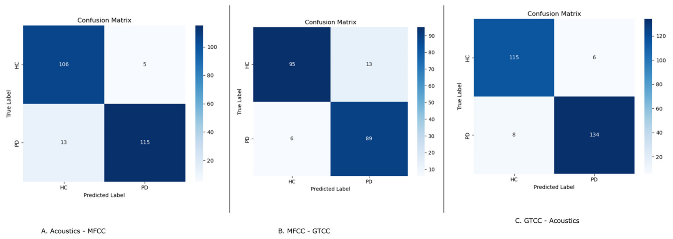
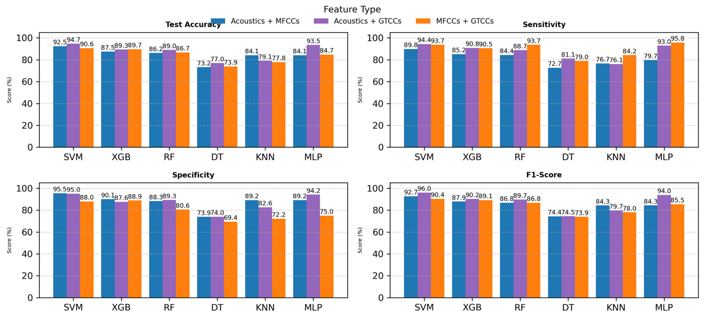
. In Figure 5 and Figure 6, we display the best-performing model’s ROC-AUC value and confusion matrix for each feature group analysis. Figure 7 compares each model’s test accuracy, sensitivity, specificity, and F1-score values.

The second experiment explored the ML model’s performance on a combination of two feature sets together. Notably, the combination of Acoustic and GTCC features with SVM yielded superior performance across almost all evaluation metrics. This configuration achieved a test accuracy of 94.68%, sensitivity of 94.37%, specificity of 95.04%, precision of 95.71%, F1-score of 96.04, ROC-AUC of 0.98, and an MCC of 0.89. Figure 5C displays the ROC-AUC for the SVM model with a combination of acoustic and GTCC values. Figure 6C illustrates a confusion matrix from the same combination of feature sets and model.

For the combination of the acoustic and MFCC feature sets, SVM showed good results, achieving a test accuracy of 92.47%, sensitivity of 89.84%, specificity of 95.50%, precision of 95.83%, F1-score of 92.74, ROC-AUC of 0.97, and an MCC of 0.75. Figure 5A displays the ROC-AUC values for the SVM model for the acoustic and MFCC values, and Figure 6A illustrates the confusion matrix.

When applied to the combination of cepstral coefficients MFCC and GTCC, the SVM model also outperformed other models and yielded a test accuracy of 90.64%, sensitivity of 93.68%, specificity of 87.96%, precision of 87.25%, F1-score of 90.36, ROC-AUC of 0.97, and an MCC of 0.81. Figure 5B and Figure 6B show the AUC values and confusion matrix of the best-performing model from the grouped MFCC and GTCC features.

Figure 7 illustrates the comparative performance using combined feature sets derived from different acoustic and cepstral representations: Acoustics, MFCCs (blue), Acoustics, GTCCs (Purple), and a combination of MFCCs with GTCCs (orange). The test accuracy, sensitivity, specificity, and F1-score are displayed across four subplots.

The test accuracy score subplot is on the top-left; the combination of GTCC cepstral features with acoustics consistently yields the best performance across most classifiers, particularly for SVM (≈94.7%) and MLP (≈93.5%). The sensitivity exhibited in the top-right plot shows that the MLP and SVM models achieve superior recall rates from a combination of cepstral features, producing the best outcomes, which are 95.8% and 93.7%, respectively.

The bottom-left subplot displays specificity, which reflects the ability to correctly identify HC. The SVM and XGB models achieved steady values for all feature combinations and showed an ability to correctly identify the negative class. The patterns in the F1-score in the bottom-right align closely with accuracy trends, with the SVM, XGB and MLP models attaining the most balanced results between precision and recall, particularly when using combined cepstral features.

These results highlight that integrating cepstral and acoustic features enhances model robustness and generalization. Among the classifiers, the XGB, MLP and SVM models consistently deliver the most reliable and high-performing results across all metrics, emphasizing the effectiveness of hybrid feature fusion acoustic and GTCCs for PD classification. These findings indicate that the fusion of complementary temporal, prosodic, and cepstral features enhances the classifier’s ability to distinguish between PD and HC effectively.

3.4. Experiment 3: All Features Combined

In the last experiment, all features were combined to train models. The results are summarized in

Table 5. ML models’ performance scores on all feature sets.

Features	Model	Train ACC	Test ACC	Sen	Spe	Pre	F1	ROC-AUC	MCC
Acoustics + MFCC + GTCC	SVM	98.60	91.92	94.30	88.24	92.55	93.42	0.98	0.83
	XGB	99.82	85.77	89.24	80.39	87.58	88.40	0.93	0.70
	RF	100	77.31	84.81	65.69	79.29	81.96	0.88	0.52
	DT	100	68.46	74.05	59.80	74.05	74.05	0.67	0.34
	KNN	95.27	80.00	81.01	78.43	85.33	83.12	0.87	0.59
	MLP	95.97	93.08	94.30	91.18	94.30	94.30	0.97	0.85

Abbreviations: SVM: Support Vector Machine; XGB: Extreme Gradient Boosting; RF: Random Forest; DT: Decision Tree; KNN: K-Nearest Neighbors; MLP: Multi-layer Perceptron; MCC: Matthew’s Correlation Coefficient; ROC-AUC: Area under the receiver operating characteristic curve; MFCCs: Mel-Frequency Cepstral Coefficients; GTCCs: Gammatone Frequency Cepstral Coefficients; ACC: Accuracy; Sen: Sensitivity; Spe: Specificity; Pre: Precision.

. Apart from the ROC-AUC and MCC values, the values are shown in percentages.

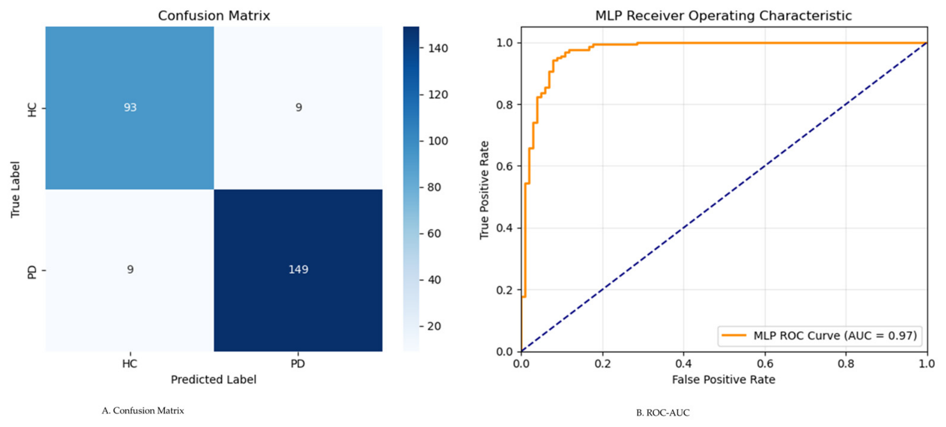
The best performance was observed with the MLP classifier. This classifier achieved a test accuracy of 93.08%, sensitivity of 94.30%, specificity of 91.18%, precision of 94.30%, F1-score of 94.30, ROC-AUC of 0.97, and an MCC of 0.85. The MLP model trained and evaluated on the combination of all feature sets consistently outperforms others in terms of sensitivity and specificity. This underlines the MLP model’s potential as a reliable tool for automatic PD detection from speech. Figure 8B represents the ROC-AUC, and Figure 8A shows the confusion matrix of the best-performing model, MLP, in this experiment.

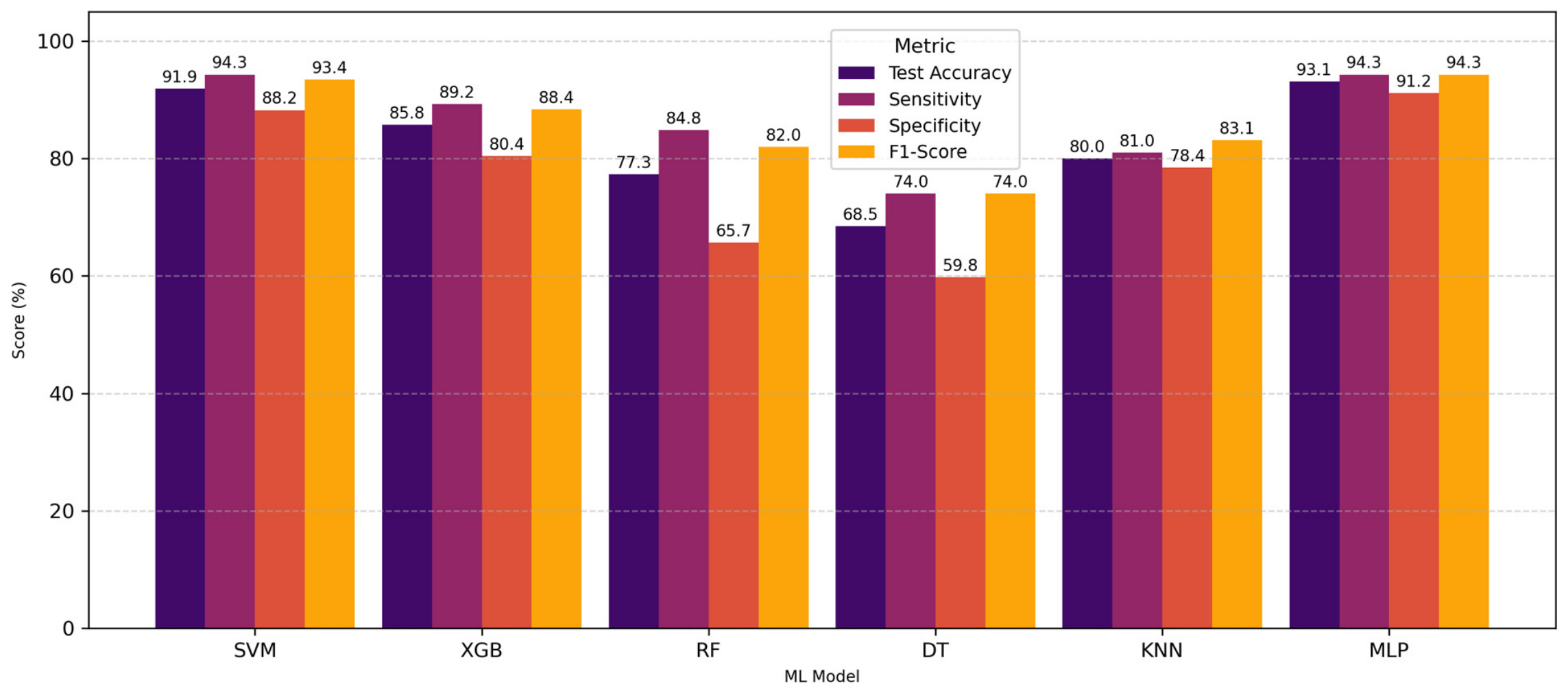
Figure 9 shows a performance analysis using the combined feature set of acoustic, MFCC, and GTCC features. The MLP model demonstrates the highest overall performance across all metrics, achieving a test accuracy of 93.1%, sensitivity of 94.3%, specificity of 91.2%, and an F1-score of 94.3%, indicating excellent generalization and balanced classification capability. The SVM model also performs competitively, with metrics consistently above 88%, showing strong stability across the evaluation criteria.

These results demonstrate that the fusion of Acoustic, MFCC, and GTCC features significantly enhances classification accuracy and reliability. Among all models, MLP achieves the most balanced and superior results, confirming its strong suitability for speech-based PD detection when using hybrid acoustic and cepstral feature representations.

4. Discussion

The primary objective of this study was to systematically evaluate the effectiveness of acoustic, Cepstral Coefficient (MFCC, GTCC), and fused feature representations for PD detection using the Italian Speech dataset. Rather than proposing a novel classification architecture, this work aimed to establish a comparative benchmark using multiple supervised classifiers within a consistent experimental framework.

In our study, the Support Vector Machine (SVM) and Multi-Layer Perceptron (MLP) models consistently achieved high classification performance across multiple feature configurations. The most effective results achieved by SVM on the acoustic with GTCC feature set yielded 94.68% accuracy, a 96.04 F1-score, 0.98 ROC-AUC, and an MCC of 0.89. Also, the MLP model demonstrated a test accuracy of 93.1%, sensitivity of 94.3%, specificity of 91.2%, and an F1-score of 94.3% in the combination of all feature sets. Our results outperform conventional ML pipelines and closely approach the results of top-performing systems in the literature.

4.1. Comparison with Existing Work

Table 6. Performance comparison of selected studies using the same dataset.

Study	Features	Classifiers	Metric
			ACC	Sen	Spe	Pre	F1	ROC-AUC	MCC
Bhatt et al. [16]	SLT	VGG16	96	97	99	99	96	N/A	N/A
Hires et al. [17]	STFT	CNN	97.81	99.14	96.53	N/A	N/A	99.41	N/A
Hires et al. [17]	MFCC	XGB	94	94.67	93.5	N/A	N/A	94.08	N/A
Malekroodi et al. [18]	STFT	VGG16	91.8	98.67	N/A	95	86.33	0.97	N/A
Amato et al. [28]	MFCC, PLP	SVM	98	100	97	98	98	1	N/A
Toye et al. [29]	MFCC	SVM	98.9	98.8	99	99.2	99	N/A	N/A
Klempír and Krupicka [30]	Wav2vec	XGB	N/A	N/A	N/A	N/A	N/A	0.98	N/A
Aversano et al. [31]	STFT	LSTM	97.1	95.2	N/A	99.2	97.1	N/A	N/A
Scimeca et al. [32]	MFCC, PLP	KNN	91.3	78.6	100	N/A	88	89.3	N/A
This study	MFCC, GTCC	MLP	93.08	94.30	91.18	94.30	94.30	0.97	0.85

Abbreviations: SVM: Support Vector Machine; XGB: Extreme Gradient Boosting; KNN: K-Nearest Neighbors; CNN: Conventional neural network; MLP: Multi-layer Perceptron; LSTM: Long Short-Term Memory; MCC: Matthew’s Correlation Coefficient; PLP: Perceptual Linear Prediction; STFT: Short-time Fourier transform; SLT: Superlet Transform; ROC-AUC: Area under the receiver operating characteristic curve; MFCCs: Mel-Frequency Cepstral Coefficients; GTCCs: Gammatone Frequency Cepstral Coefficients; ACC: Accuracy; Sen: Sensitivity; Spe: Specificity; Pre: Precision: N/A: Not ava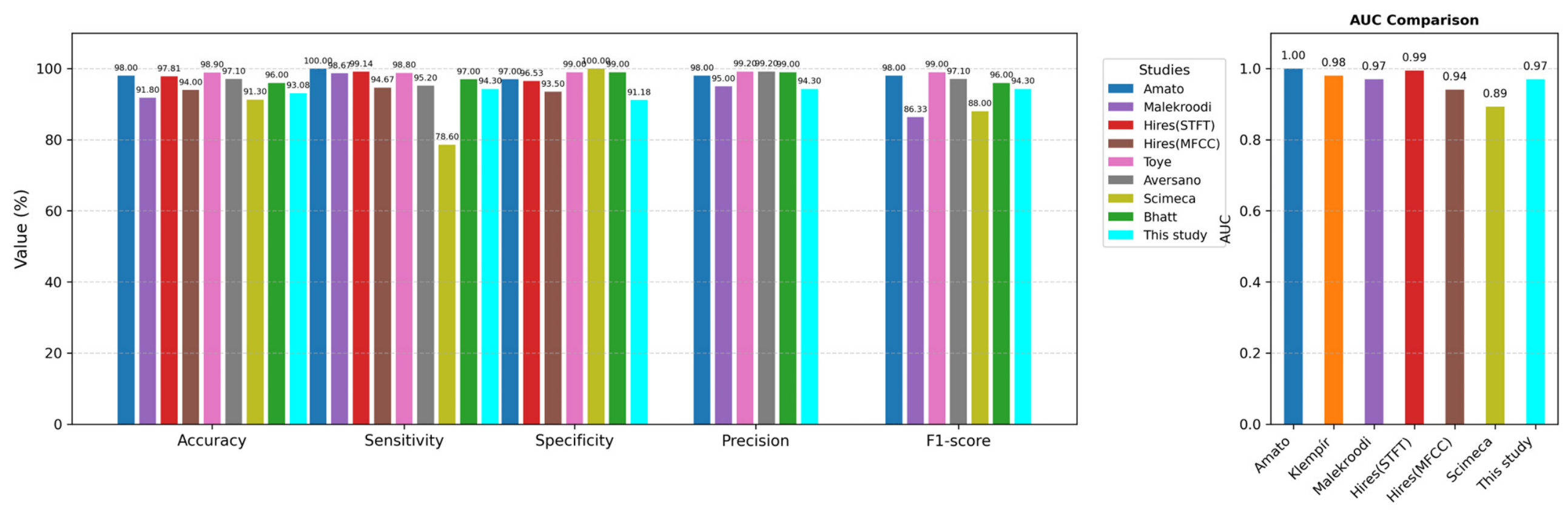ilable.

compares the results of selected previous studies. However, direct comparison between studies remains challenging due to differences in data preprocessing, feature extraction methods, and validation strategies. In Figure 10, we also show graphical bar chart comparisons of the results of each study using the IPVS dataset.

Several previous studies have reported exceptionally high performance using the same datasets and modeling approaches. For example, Amato et al. [28] utilized MFCC and PLP features with SVM, achieving an impressive 98% accuracy and high sensitivity (100%) with an ROC-AUC of 1.0. Similarly, Toye et al. [29] reported 98.9% accuracy and 99.2% precision using SVM on MFCC-based features. However, both studies rely heavily on spectral features (MFCCs and PLPs), which may be sensitive to environmental noise or speaker variability.

Hires et al. [17] demonstrated superior results using CNNs and STFT-based spectrograms, achieving up to 97.81% accuracy and an ROC-AUC of 99.41. Their work, along with that of Malekroodi et al. [18], confirms the viability of deep learning with time-frequency image representations (e.g., STFT) for robust PD detection. However, our study achieved comparable performance using traditional handcrafted features and a simple architecture such as SVM. This suggests that deep learning is not strictly necessary for high diagnostic accuracy, especially when informative ear-specific acoustic features like GTCCs are employed.

Bhatt et al. [16] and L. Aversano et al. [31] also obtained high performance by using CNN- and LSTM-based architectures applied to time–frequency spectrograms. Notably, Bhatt et al. [16] employed Superlet Transforms (SLT) to generate high-resolution spectrograms, reporting 96% accuracy and exceptional sensitivity and specificity values. Aversano et al. [31], using an LSTM architecture, reported 97.1% accuracy. This reinforces the growing consensus around sequential DL models for modeling speech dynamics under neurodegenerative conditions.

On the other hand, Klempír and Krupicka [30] explored more recent representation learning techniques using Wav2Vec embeddings, attaining a high ROC-AUC of 0.98. While such embedding-based approaches offer language-agnostic representations and improved scalability, they often require substantial computational resources and larger datasets for fine-tuning, which may not always be feasible in clinical settings.

Compared with previous studies, our results are competitive while maintaining methodological transparency through subject-wise data partitioning and systematic evaluation of multiple feature representations. More importantly, the present work provides a unified comparison of acoustic, MFCC, GTCC, and fused feature sets under identical experimental conditions, allowing the relative contribution of each feature representation to be assessed more reliably.

4.2. Strengths and Implications

A notable finding of this study is the consistent contribution of GTCC features across multiple classification models. While MFCCs remain the most widely used cepstral representation in speech-based PD detection, GTCCs employ a Gammatone filter bank that more closely models human auditory perception. The results indicate that GTCC features capture complementary information that may enhance discrimination between PD and HC speech, particularly when combined with conventional acoustic descriptors.

Another important finding is the benefit of feature fusion. Across several classifiers, fused feature sets generally outperformed individual feature groups, suggesting that different speech representations capture distinct aspects of PD-related vocal impairment. In particular, the combination of acoustic and GTCC features yielded the most robust and consistent performance.

From a practical perspective, the use of interpretable handcrafted speech features and computationally efficient machine learning algorithms offers a favorable balance between predictive performance and implementation complexity. Such approaches may be attractive for future speech-based screening tools and decision-support systems, particularly in resource-constrained environments where computational efficiency and model interpretability are important considerations.

4.3. Limitations and Future Directions

Although this study’s results are encouraging, several limitations should be acknowledged. First, this study was conducted using a single publicly available dataset and focused exclusively on binary classification between PD and healthy controls. Consequently, the findings should be interpreted as a dataset-specific benchmark rather than definitive evidence of clinical generalizability. Although subject-wise partitioning and independent testing were employed to reduce data leakage and overfitting, external validation on independent datasets was not performed due to the size of the dataset and remains necessary to establish model robustness across different populations and recording conditions.

The relatively limited dataset size may restrict model generalization. Larger and more diverse datasets would better capture variability across speakers, demographic factors, recording conditions, and disease stages. Future work will therefore focus on combining multiple publicly available PD speech datasets and conducting cross-dataset evaluations to assess model performance under more realistic and heterogeneous conditions.

The IPVS dataset contains an inherent age imbalance, where healthy control recordings include both young and adult participants, whereas PD participants are predominantly older adults. Although demographic variables were not included as model inputs, acoustic features may still indirectly capture age-related speech characteristics. Therefore, part of the discriminative information learned by the classifiers may reflect age-associated vocal variability rather than PD-specific pathology. Future studies should employ age-matched cohorts or statistically controlled experimental designs to better isolate disease-related speech biomarkers.

Another limitation is the absence of disease severity and longitudinal information within the dataset. The current analysis is restricted to the detection of PD versus HC and does not evaluate disease staging, progression monitoring, or treatment-related changes in speech. Future studies should incorporate datasets containing clinical severity measures and longitudinal recordings to investigate the potential of speech biomarkers for monitoring disease progression and supporting personalized patient management.

Furthermore, the present study did not include prospective clinical evaluation or real-world deployment testing. While the proposed framework relies on computationally efficient handcrafted features and conventional machine learning classifiers that are suitable for practical implementation, its performance has only been assessed under controlled research conditions. Prospective studies involving real-world clinical recordings are required to evaluate robustness in the presence of environmental noise, recording-device variability, and operational constraints encountered in healthcare settings.

Future work will focus on external validation and cross-dataset evaluation using both the IPVS dataset and the English-language MDVR-KCL dataset. Training and testing across different datasets, languages, and recording conditions will provide a more rigorous assessment of model generalizability. Additional directions include multilingual speech analysis, longitudinal monitoring of disease progression, and comparison with contemporary deep-learning architectures. In addition, the development of real-time speech acquisition and automated analysis pipelines will be explored to facilitate integration into clinical decision-support systems. These efforts will contribute toward establishing robust, scalable, and clinically applicable speech-based biomarkers for Parkinson’s disease detection and monitoring.

5. Conclusions

This study presents a comprehensive evaluation of speech/voice-based machine learning approaches for the automatic detection of PD using the native Italian Voice and Speech dataset. By extracting a diverse set of acoustic features, including perturbation, prosodic and temporal features, MFCC, and GTCC descriptors, and systematically evaluating their diagnostic relevance across multiple classification models, we have demonstrated that speech-based biomarkers can serve as reliable indicators of PD-related motor speech impairments.

The results demonstrated that both feature representation and classifier selection substantially influence classification performance. Among the evaluated configurations, the combination of acoustic and GTCC features achieved the strongest overall performance, with the Support Vector Machine (SVM) classifier producing the best results. These findings indicate that GTCC features provide complementary information to conventional acoustic descriptors and may enhance the discrimination of PD and healthy control speech.

Rather than proposing a novel classification architecture, this work provides a comparative benchmark of acoustic, MFCC, GTCC, and fused feature representations within a consistent experimental framework. The results contribute to a better understanding of the relative effectiveness of these feature sets and highlight the potential value of GTCC-based representations in speech-based PD analysis.

Several limitations should be considered when interpreting the findings. The study was conducted on a single publicly available dataset, employed a binary classification framework, and may be influenced by demographic characteristics inherent to the dataset. Therefore, the reported performance should be viewed as a dataset-specific benchmark rather than definitive evidence of clinical generalizability.

Future work will focus on external validation using independent datasets, cross-lingual evaluation between Italian and English speech corpora, age-matched study designs, and comparison with contemporary deep-learning approaches. Such investigations will help establish the robustness, generalizability, and clinical utility of speech-based biomarkers for Parkinson’s disease detection.

References

- Tolosa, E.; Garrido, A.; Scholz, S.W.; Poewe, W. Challenges in the Diagnosis of Parkinson’s Disease. Lancet Neurol. 2021, 20, 385–397. [Google Scholar] [CrossRef] [PubMed]
- Kalia, L.V.; Lang, A.E. Parkinson’s Disease. Lancet 2015, 386, 896–912. [Google Scholar] [CrossRef] [PubMed]
- Hayes, M.T. Parkinson’s Disease and Parkinsonism. Am. J. Med. 2019, 132, 802–807. [Google Scholar] [CrossRef] [PubMed]
- Sapmaz Atalar, M. Hypokinetic Dysarthria in Parkinson’s Disease: A Narrative Review. Med. Bull. Sisli Hosp. 2023, 57, 163–170. [Google Scholar] [CrossRef] [PubMed]
- Moya-Galé, G.; Levy, E.S. Parkinson’s Disease-Associated Dysarthria: Prevalence, Impact and Management Strategies. Res. Rev. Park. 2019, 9, 9–16. [Google Scholar] [CrossRef]
- Ho, A.K.; Iansek, R.; Marigliani, C.; Bradshaw, J.L.; Gates, S. Speech Impairment in a Large Sample of Patients with Parkinson’s Disease. Behav. Neurol. 1999, 11, 131–137. [Google Scholar] [CrossRef] [PubMed]
- Rusz, J.; Cmejla, R.; Ruzickova, H.; Ruzicka, E. Quantitative Acoustic Measurements for Characterization of Speech and Voice Disorders in Early Untreated Parkinson’s Disease. J. Acoust. Soc. Am. 2011, 129, 350–367. [Google Scholar] [CrossRef] [PubMed]
- Little, M.A.; McSharry, P.E.; Hunter, E.J.; Spielman, J.; Ramig, L.O. Suitability of Dysphonia Measurements for Telemonitoring of Parkinson’s Disease. IEEE Trans. Biomed. Eng. 2009, 56, 1015–1022. [Google Scholar] [CrossRef] [PubMed]
- Tsanas, A.; Little, M.A.; McSharry, P.E.; Spielman, J.; Ramig, L.O. Novel Speech Signal Processing Algorithms for High-Accuracy Classification of Parkinsons Disease. IEEE Trans. Biomed. Eng. 2012, 59, 1264–1271. [Google Scholar] [CrossRef] [PubMed]
- Postuma, R.B.; Berg, D.; Stern, M.; Poewe, W.; Olanow, C.W.; Oertel, W.; Obeso, J.; Marek, K.; Litvan, I.; Lang, A.E.; et al. MDS Clinical Diagnostic Criteria for Parkinson’s Disease. Mov. Disord. 2015, 30, 1591–1601. [Google Scholar] [CrossRef] [PubMed]
- Jankovic, J. Parkinson’s Disease: Clinical Features and Diagnosis. J. Neurol. Neurosurg. Psychiatry 2008, 79, 368–376. [Google Scholar] [CrossRef] [PubMed]
- Arora, S.; Venkataraman, V.; Zhan, A.; Donohue, S.; Biglan, K.M.; Dorsey, E.R.; Little, M.A. Detecting and Monitoring the Symptoms of Parkinson’s Disease Using Smartphones: A Pilot Study. Park. Relat. Disord. 2015, 21, 650–653. [Google Scholar] [CrossRef] [PubMed]
- Van Gelderen, L.; Tejedor-García, C. Innovative Speech-Based Deep Learning Approaches for Parkinson’s Disease Classification: A Systematic Review. Appl. Sci. 2024, 14, 7873. [Google Scholar] [CrossRef]
- Maryn, Y.; Corthals, P.; Van Cauwenberge, P.; Roy, N.; De Bodt, M. Toward Improved Ecological Validity in the Acoustic Measurement of Overall Voice Quality: Combining Continuous Speech and Sustained Vowels. J. Voice 2010, 24, 540–555. [Google Scholar] [CrossRef] [PubMed]
- El Ayadi, M.; Kamel, M.S.; Karray, F. Survey on Speech Emotion Recognition: Features, Classification Schemes, and Databases. Pattern Recognit. 2011, 44, 572–587. [Google Scholar] [CrossRef]
- Bhatt, K.; Jayanthi, N.; Kumar, M. High-Resolution Superlet Transform Based Techniques for Parkinson’s Disease Detection Using Speech Signal. Appl. Acoust. 2023, 214, 109657. [Google Scholar] [CrossRef]
- Hireš, M.; Drotár, P.; Pah, N.D.; Ngo, Q.C.; Kumar, D.K. On the Inter-Dataset Generalization of Machine Learning Approaches to Parkinson’s Disease Detection from Voice. Int. J. Med. Inform. 2023, 179, 105237. [Google Scholar] [CrossRef] [PubMed]
- Malekroodi, H.S.; Madusanka, N.; Lee, B.-i.; Yi, M. Leveraging Deep Learning for Fine-Grained Categorization of Parkinson’s Disease Progression Levels through Analysis of Vocal Acoustic Patterns. Bioengineering 2024, 11, 295. [Google Scholar] [CrossRef] [PubMed]
- Sakar, B.E.; Isenkul, M.E.; Sakar, C.O.; Sertbas, A.; Gurgen, F.; Delil, S.; Apaydin, H.; Kursun, O. Collection and Analysis of a Parkinson Speech Dataset with Multiple Types of Sound Recordings. IEEE J. Biomed. Health Inform. 2013, 17, 828–834. [Google Scholar] [CrossRef] [PubMed]
- Verde, L.; De Pietro, G.; Sannino, G. Voice Disorder Identification by Using Machine Learning Techniques. IEEE Access 2018, 6, 16246–16255. [Google Scholar] [CrossRef]
- Dimauro, G.; Di Nicola, V.; Bevilacqua, V.; Caivano, D.; Girardi, F. Assessment of Speech Intelligibility in Parkinson’s Disease Using a Speech-to-Text System. IEEE Access 2017, 5, 22199–22208. [Google Scholar] [CrossRef]
- Dimauro, G.; Caivano, D.; Bevilacqua, V.; Girardi, F.; Napoletano, V. VoxTester, Software for Digital Evaluation of Speech Changes in Parkinson Disease. In Proceedings of the 2016 IEEE International Symposium on Medical Measurements and Applications, MeMeA 2016—Proceedings, Benevento, Italy, 15–18 May 2016. [Google Scholar] [CrossRef]
- IEEE DataPort. Italian Parkinson’s Voice and Speech. Available online: https://ieee-dataport.org/open-access/italian-parkinsons-voice-and-speech (accessed on 6 August 2025).
- Sainburg, T.; Thielk, M.; Gentner, T.Q. Finding, Visualizing, and Quantifying Latent Structure across Diverse Animal Vocal Repertoires. PLoS Comput. Biol. 2020, 16, e1008228. [Google Scholar] [CrossRef] [PubMed]
- Sainburg, T. Timsainb/Noisereduce, version V1.0; GitHub: San Francisco, CA, USA, 2019.
- Jadoul, Y.; de Boer, B.; Ravignani, A. Parselmouth for Bioacoustics: Automated Acoustic Analysis in Python. Bioacoustics 2024, 33, 1–19. [Google Scholar]
- Robert, J.; Webbie, M. Pydub; PyPI: Beaverton, OR, USA, 2018. [Google Scholar]
- Amato, F.; Borzi, L.; Olmo, G.; Artusi, C.A.; Imbalzano, G.; Lopiano, L. Speech Impairment in Parkinson’s Disease: Acoustic Analysis of Unvoiced Consonants in Italian Native Speakers. IEEE Access 2021, 9, 166370–166381. [Google Scholar] [CrossRef]
- Toye, A.A.; Kompalli, S. Comparative Study of Speech Analysis Methods to Predict Parkinson’s Disease. arXiv 2021, arXiv:2111.10207. [Google Scholar]
- Klempíř, O.; Krupička, R. Analyzing Wav2Vec 1.0 Embeddings for Cross-Database Parkinson’s Disease Detection and Speech Features Extraction. Sensors 2024, 24, 5520. [Google Scholar] [CrossRef] [PubMed]
- Aversano, L.; Bernardi, M.L.; Cimitile, M.; Iammarino, M.; Montano, D.; Verdone, C. A Machine Learning Approach for Early Detection of Parkinson’s Disease Using Acoustic Traces. In Proceedings of the 2022 IEEE International Conference on Evolving and Adaptive Intelligent Systems (EAIS); IEEE: New York, NY, USA, 2022; pp. 1–8. [Google Scholar]
- Scimeca, S.; Amato, F.; Olmo, G.; Asci, F.; Suppa, A.; Costantini, G.; Saggio, G. Robust and Language-Independent Acoustic Features in Parkinson’s Disease. Front. Neurol. 2023, 14, 1198058. [Google Scholar] [CrossRef] [PubMed]
Figure 1.
Workflow of ML-based PD and HC classifications using IPVS voice dataset.
Figure 2.
Best-performing model’s ROC-AUC on individual features. Abbreviations: SVM: Support Vector Machine; MFCCs: Mel-Frequency Cepstral Coefficients; GTCCs: Gammatone Frequency Cepstral Coefficients; AUC: Area under the Curve.
Figure 3.
Confusion matrix of best-performing SVM model for PD and HC classifications. Abbreviations: MFCCs: Mel-Frequency Cepstral Coefficients; GTCCs: Gammatone Frequency Cepstral Coefficients; HC: Healthy Control; PD: Parkinsons’s Disease.
Figure 4.
ML models’ performance on individual feature sets. Abbreviations: SVM: Support Vector Machine; XGB: Extreme Gradient Boosting; RF: Random Forest; DT: Decision tree; KNN: K-Nearest Neighbors; MLP: Multilayer Perceptron; MFCCs: Mel-Frequency Cepstral Coefficients; GTCCs: Gammatone Frequency Cepstral Coefficients.
Figure 5.
Best ROC-AUC on paired feature combinations. Abbreviations: SVM: Support Vector Machine; MFCCs: Mel-Frequency Cepstral Coefficients; GTCCs: Gammatone Frequency Cepstral Coefficients; AUC: Area under the Curve.
Figure 6.
Best model’s confusion matrix for feature combination sets. Abbreviations: MFCCs: Mel-Frequency Cepstral Coefficients; GTCCs: Gammatone Frequency Cepstral Coefficients; HC: Healthy Control; PD: Parkinsons’s Disease.
Figure 7.
ML models’ performance with a combination of two sets of features. Abbreviations: SVM: Support Vector Machine; XGB: Extreme Gradient Boosting; RF: Random Forest; DT: Decision tree; KNN: K-Nearest Neighbors; MLP: Multilayer Perceptron; MFCCs: Mel-Frequency Cepstral Coefficients; GTCCs: Gammatone Frequency Cepstral Coefficients.
Figure 8.
Best-performing model confusion matrix (A) and ROC-AUC (B).
Figure 9.
ML model performance comparison with three types of feature combinations. Abbreviations: SVM: Support Vector Machine; XGB: Extreme Gradient Boosting; RF: Random Forest; DT: Decision Tree; KNN: K-Nearest Neighbors; MLP: Multi-layer Perceptron.
Figure 10.
Comparison of the performance of this work and previous studies. The left-side subfigure shows a comparison of study metrics: accuracy, sensitivity, specificity, precision, and F1-score. The right-side subplot illustrates an AUC (area under the curve) value comparison. This study’s values are shown in a sky blue color.