Homogenization Methods of Lattice Materials

Definition

The existing methods for analyzing the behaviors of lattice materials require high computational power. The homogenization method is the alternative way to overcome this issue. Homogenization is an analysis to understand the behavior of an area of lattice material from a small portion for rapid analysis and precise approximation. This paper provides a summary of some representative methodologies in homogenization.

1. Introduction

The homogenization approach is based on the idea that the properties of a heterogeneous medium can be determined by analyzing a small portion of it [1]. In other words, Representative Volume Element (RVE) is a sample for the entire area. It needs to be underlined that the RVE includes the micro-structural property of effective materials and expands to the global domain, where uniformly applied strain or stress exists with a boundary condition [1,2,3], which does not require extensive and full-scale simulations. Meanwhile, this strategy is only applicable when the homogeneities are dual orders of magnitude that are below the effective medium’s characteristic length [1,2,3].

The idea of lattice material homogenization is represented where the RVE is a square unit cell. A body Ω with a periodic lattice with a t at the traction boundary ${\mathsf{\Gamma }}_t$, a displacement d at the displacement boundary ${\mathsf{\Gamma }}_d$, and a body force f is inserted by a homogenized body $\overline{\mathsf{\Omega }}$. The mechanical properties of RVE are to be determined by the macroscopic behavior of Ω and $\overline{\mathsf{\Omega }}$ are equivalent [1].

2. Homogenization Methods

In homogenization methods, the relative density is one of the key material properties, and it is defined density ratio of lattice material to solid ($\overline{\rho }={\rho }^{\ast }/{\rho }_s)$ and it plays an essential role in determining a lattice’s elastostaticity. The relation between relative density and relative modulus is explained and applied in Figure 1. Slope 1 in Figure 2 is lattice design in the behavior of stretching and slope 2 for bending. Honeycomb is one of the most commonly used sandwich panel cores and is highly efficient. Relative density physically represents the porosity. A relative density number in a low region suggests high 1-porosity, whereas a high value is low. For example, $\overline{\rho }=1$ represents 0% porosity since the density is the same as a solid. As a result, it is critical to use a homogenization method based on the relative density. When low relative density dominates, e.g., $\overline{\rho }<0.3$, using Euler–Bernoulli or Timoshenko beam to represent cell wall deformation yields accurate results [4,5,6,7]. Moreover, micro-polar theory [8], Bloch wave analysis [9], and Cauchy–Born hypothesis could be adopted, too. Finally, the AH (asymptotic homogenization) approach produces a more accurate result [10]. In this article, most representative techniques for homogenization are introduced for readers of interest.

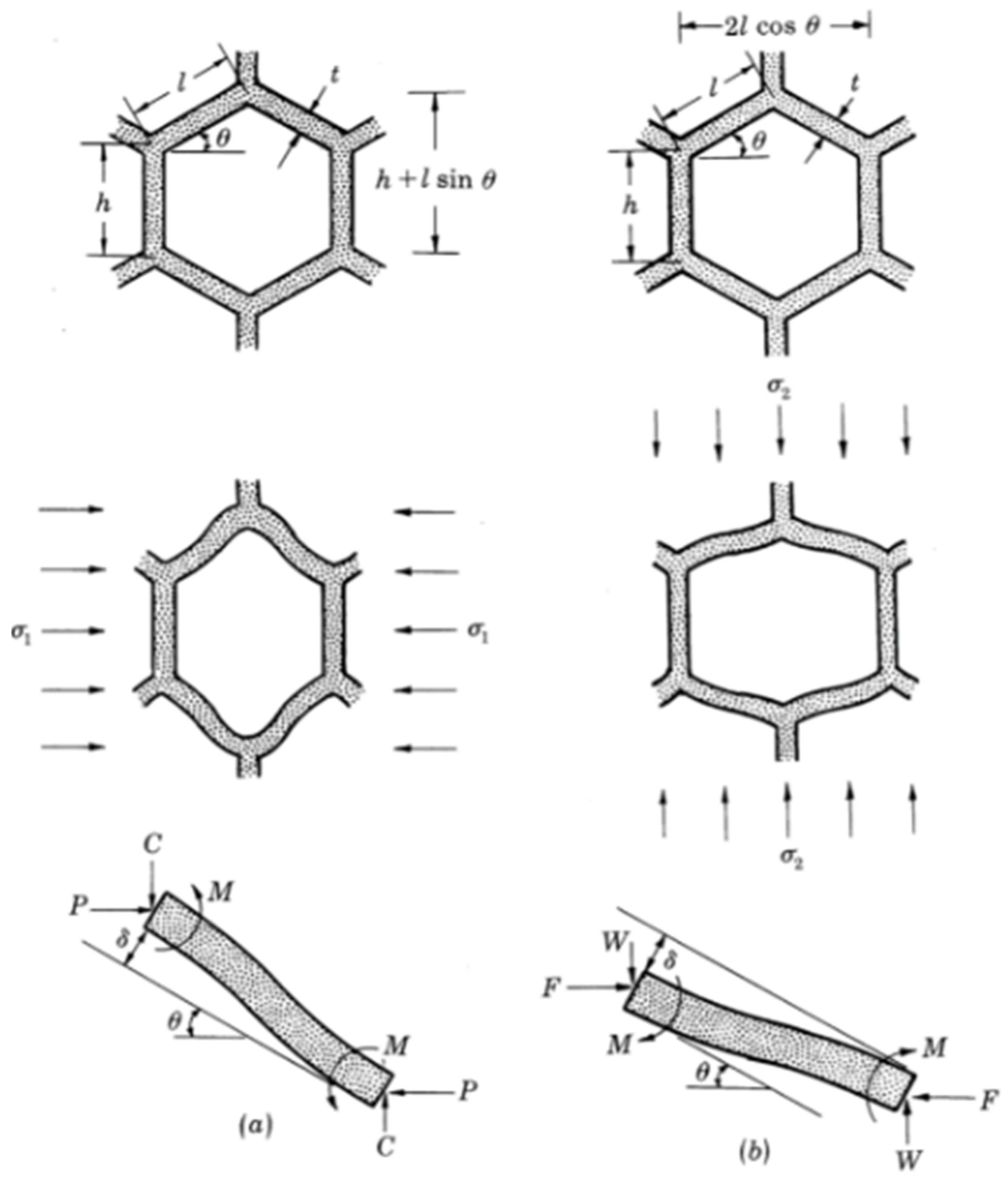
2.1. Beam Theory Approach

The force-based one is another term for the beam theory approach [1]. It is appropriate when simulating cell wall deformation for a single unit. The field quantity from the unit cell is presumed uniform over the RVE. Analytical closed-form equations for the mechanical properties of various shapes and geometry have been studied over the years [4,5,7]. Christensen [12] also gave a comprehensive review of the approach.

Gibson and Ashby initialized the study of cellular structures and honeycomb topologies [4]. First, they analyzed honeycomb using beam theory on a unit cell, as shown in Figure 3. Furthermore, they suggested a closed-form solution for the mechanical properties of honeycomb and verified it through experiments. Later, Masters and Evans [7] went a step further by incorporating three mechanisms into their model: flexure, stretching, and hinging. As a result, they could obtain a broader expression for characteristics. Then, Wang and Mcdowell [5] studied honeycomb architectures of seven different cell types and looked at in-plane shear properties.

The most significant advantage of this is closed-form mathematical formulas’ mechanical characteristics. Assuming the cell wall is a beam, the following uses are restricted: For starters, this approach is only applicable to cases with a low relative density ($\overline{\rho }<0.3$). Second, because Euler’s beam assumes strains are small and large deformation does not occur, this approach cannot be adopted when nonlinearities exist or the geometry has a complicated topology.

2.2. Strain Energy Equivalence

The strain energy equivalence method employs an application of the RVE concept directly. This method determines the performance of the macroscopic medium solely by the RVE’s mechanical behavior. The averages of particular mechanical properties regarding the volume’s surface are equal to obtain the equivalent condition of the effective medium and its RVE [13]. Then, the effective medium’s constitutive equation and its related RVE must be solved considering the constraint of both volume elements is fulfilled.

The first approach is the surface average [1]. This applies stress or strain distributions to the RVE surface. Therefore, the stress distribution on the RVE is to be equivalent to the stress distribution in the volume of the effective medium if

$${{\displaystyle \int }}_{{\mathsf{\Gamma }}_{\mathrm{RVE}}^i}{T}_{i}d{\mathsf{\Gamma }}_{RVE}={{\displaystyle \int }}_{{\mathsf{\Gamma }}_{\mathrm{RVE}}^i}{T}_i^{\ast }d{\mathsf{\Gamma }}_{RVE}$$

(1)

satisfies, where $T_i^{\ast }$ is the traction vector on the RVE surface and ${\mathsf{\Gamma }}_{RVE}^i$ is a part of its boundary, parallel to one of the coordinate planes. The second condition lies between the strain tensor in the effective medium and the RVE, which is expressed

$$\overline{{ϵ}_{ij}}=\overline{{ϵ}_{ij}^{\ast }}$$

(2)

Furthermore, for a volume element, the mesoscopic strain is expressed

$$\overline{ϵ}=\frac{1}{2}\frac{1}{V}{{\displaystyle \int }}_{{\mathsf{\Gamma }}_{RVE}}\left(u_i{n}_j+u_j{n}_i\right) d{\mathsf{\Gamma }}_{RVE}$$

(3)

The equivalence condition in Equation (2) is between the strain tensor generated in the effective medium and its RVE. Furthermore, for a volume element of general shape, the mesoscopic strain can be expressed as shown in Equation (3), where $V$ is the RVE volume and $n_i$ are the components of the normal vector on ${\mathsf{\Gamma }}_{RVE}$, and $u_{ii}$ are tensors. Equations (2) and (3) state that the surface integral over the RVE of the quantity $\left(u_i{n}_j+u_j{n}_i\right)$ has to be equal to both volume elements.

The surface average method comes with a major shortcoming. The surface average approach produces mistakes in estimating the effective strain energy for more complex geometry, such as non-orthotropic geometry. This mistake is caused by coupled stress exerted on the intersections of the cell walls and the RVE surfaces. A volume average strategy can be utilized to avoid this difficulty. This approach is rooted in the assumption that the microscopic scaled behavior in the RVE and its medium is considered equivalent if the RVE strain energy equals the effective medium, and this can be expressed as

$$\overline{w}=\frac{1}{V}{{\displaystyle \int }}_{{\mathsf{\Omega }}_{RVE}}wd{\mathsf{\Omega }}_{RVE}=\frac{1}{V}{{\displaystyle \int }}_{{\mathsf{\Omega }}_{RVE}}{w}^{\ast }d{\mathsf{\Omega }}_{RVE}=\overline{w^{\ast }}$$

(4)

where $w$ is the strain energy density distribution and ${\mathsf{\Omega }}_{RVE}$ is the RVE area. Therefore, the strain equivalence condition, $\overline{{ϵ}_{ij}}$ is written as

$$\overline{{ϵ}_{ij}}=\frac{1}{V}{{\displaystyle \int }}_{{\mathsf{\Omega }}_{RVE}}{ϵ}_{ij} d{\mathsf{\Omega }}_{RVE}=\frac{1}{V}{{\displaystyle \int }}_{{\mathsf{\Omega }}_{RVE}}{ϵ}_{ij}^{\ast } d{\mathsf{\Omega }}_{RVE}=\overline{{ϵ}_{ij}^{\ast }}$$

(5)

Strain energy equivalency has been used in various types of cellular structures, including sandwich and corrugated structures [13,14,15,16,17]. The benefit is its direct relativity to the fundamental rules of continuum mechanics and energy conservation. Furthermore, there are no restrictions on using this technology in terms of cellular structural geometries and unit cell topologies.

2.3. Micropolar Theory

Classical continuum mechanics and theory are not applicable when discontinuities or significant strain gradients exist in the domain, such as fracture tips or notches. E. and F. Cosserat [18] and Eringen [19] introduced the micropolar theory, commonly referred to as Cosserat theory, to generalize classical continuum theory. The micropolar theory adds a microscopic rotation to translational deformations, and its key premise is that a point’s displacement and rotation are independent kinematic features. This indicates that, in a lattice material, both the joint displacement and rotation contribute to total joint displacement. Its kinematic relations in linear micropolar elasticity theory are stated below in Equations (6) and (7).

$${ϵ}_{ij}\mid =u_{j,i }-e_{kij}{\varphi }_k$$

(6)

$$k_{ij}\mid ={\varphi }_{j,i }$$

(7)

where $u_{j,i}$ is the displacement gradient, ${ϵ}_{ij}$ is the strain, ${\varphi }_k$ is the microrotation, $k_{ij}$ is the curvature strain, and ${\varphi }_{j,i}$ is the microrotation gradient. The generalized strain vector of a micropolar medium is expressed as follows.

$$ϵ={\left[{ϵ}_{11} {ϵ}_{22} {ϵ}_{12} {ϵ}_{21} k_{13} k_{23}\right]}^T={\left[u_{1,1} u_{2,2} u_{2,1}-\varphi u_{1,2}+\varphi {\varphi }_{3,1}{\varphi }_{3,2}\right]}^T$$

(8)

The generalized stress vector is provided below in Equation (9).

$$\sigma ={\left[{\sigma }_{11} {\sigma }_{22} {\sigma }_{12} {\sigma }_{21} m_{13} m_{23}\right]}^T$$

(9)

where $m_{13}$ and $m_{23}$ are the couple stresses in the $x$ and $y,$ and the 2D constitutive relations for anisotropic micropolar solids are as below.

$$\sigma =\overline{C}ϵ$$

(10)

where $\overline{C}$ is the $6\times 6$ matrix of the constitutive law coefficients.

The coefficients of the constitutive equations, $\overline{C}$, must be found to characterize a cellular structure as a micropolar continuum. The stiffness matrix’s micropolar elastic constants are found through structural analysis of the unit cell [8] or an energy approach [20]. The beam theory approach can analyze the unit cell to derive the general deformational RVE states. Constitutive equations can calculate the effective stress and strain over the RVE. The cell stresses can be derived using the energy approach by deriving the strain energy density of the strain vector.

Micropolar theory with beam theory approach/energy approach has shown several shortcomings: (1) It could be applied only to unit cells with limited shapes containing a single joint at the center or the unit cell, and (2) the new micropolar variable is an additional degree of freedom. Therefore, an additional step is necessary to solve the governing equations.

2.4. Solid-State Physics Approach: Bloch’s Theorem and Cauchy Born Hypothesis

Because of their similarities, the concepts of solid-state physics and solid mechanics can be used to examine the properties of lattice structures. From the solid-state physics perspective, lattice arrangement is a periodic arrangement of points. The space is tessellated if the period of unit cells is stacked in two or three dimensions. The base is the mathematical representations of physical quantities repeated in each cell translation [9]. The preceding definition can define a lattice material in continuum mechanics.

Bloch wave analysis and the Cauchy–Born hypothesis are solid-state physics approaches that may be utilized to explore the behavior of lattice materials in solid mechanics [9,21]. Bloch’s theorem was initially created to describe electron particle transit within a solid’s crystal structure. Bloch’s theorem could then investigate the wave function propagation through an infinite lattice construction. The Cauchy–Born hypothesis [22], on the other hand, analyzes the macroscopic mechanism from an applied strain [1] and states that the infinitesimal displacement of a periodic lattice pattern is composed of two parts, namely the deformation from a macroscopic strain field and the periodic displacement of a unit cell. Bloch’s theorem clarifies and defines the wave function propagation over an infinite lattice structure.

The Cauchy–Born hypothesis could not be applied to the kinematic compatibility relation for the unit cell without the use of the Dummy node technique [9]. Earlier work has extensively studied this process and the method’s more detailed derivation [9,23,24,25] and will not be addressed here. This method was studied and developed assuming cell walls to be beam elements. As a result, these assumptions, such as those of the elasticity theory approach, limit their applications to low relative density regions ($\overline{\rho }<0.3$).

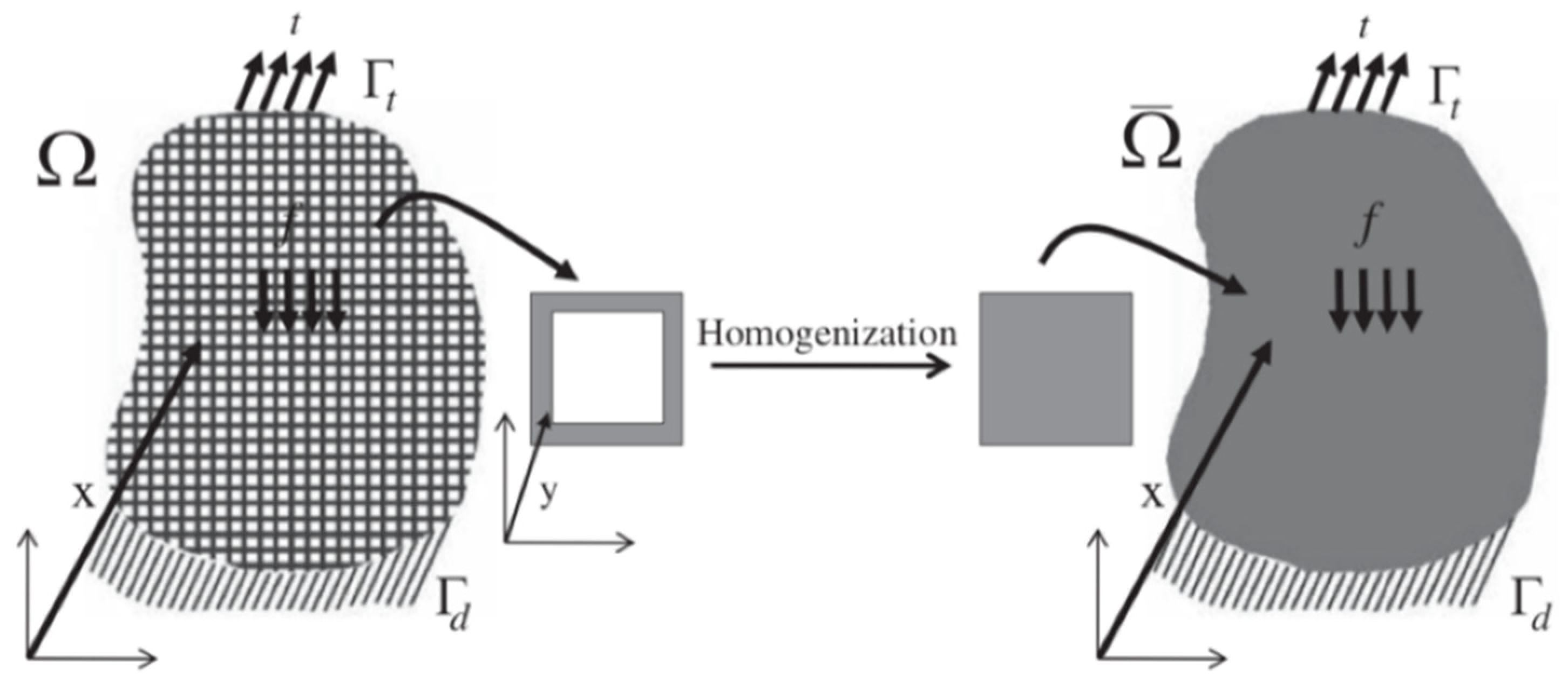
2.5. Asymptotic Homogenization Approach

In the application of broader scenarios, analytical solutions have revealed some limits. As a result, the asymptotic homogenization (AH) theorem is one of the more well-developed theories with solid mathematical foundations that have been effectively utilized to predict mechanical properties in porous materials [26]. This method has been tested using experimental data and demonstrated to be one of the most dependable and accurate methods [27]. Arabnejad et al. conducted considerable research on the use of AH to acquire mechanical parameters of the lattice materials/structure [10].

The core premise of AH is each quantity relies on two different scales: one is on the macroscopic level x and the other on microscopic, y = x/𝜖 where 𝜖 is a ratio of sizes of RVE and the macroscopic medium and signifies that stress or strain will fluctuate quicker by 1/𝜖. The AH also assumes the field quantities fluctuate smoothly at macroscopic levels and follow periodic patterns at the microscale. From the AH, each mechanical variable, such as the displacement field, u could be expanded into a power series with respect to 𝜖 is below in Equation (11).

$$u^{ϵ}=u_0\left(x,y\right)+ϵu_1\left(x,y\right)+{ϵ}^2{u}_2\left(x,y\right)+\dots$$

(11)

$u_1$ and $u_2$ are displacement perturbations due to the microstructure, and $u_0$ The average value of the displacement field relies only on the macroscopic scale [26]. Taking the derivative of the power series, we obtain below.

$$\frac{du}{dx}=ϵ\left(u\right)\mid =\frac{1}{2}{\left(\nabla u_0^T+\nabla u_0\right)}_x+\frac{1}{2}{\left(\nabla u_1^T+\nabla u_1\right)}_y+O\left(ϵ\right)$$

(12)

$$ϵ\left(u\right)\mid = \left\{\overline{ϵ}\left(u\right)\right\} + \left\{{ϵ}^{\ast }\left(u\right)\right\}$$

(13)

where $\overline{ϵ}\left(u\right)$ is the macroscopic level strain, and $ϵ\ast \left(u\right)$ is the microscopic fluctuating strain. Note that $O\left(ϵ\right)$ and higher terms are neglected here. Substitute the above into the equilibrium equation for a cellular body ${\mathsf{\Omega }}^{ϵ}$ and that leads to Equation (14) as below [26].

$${{\displaystyle \int }}_{{\mathsf{\Omega }}^{ϵ}}{C}_{ijkl}\left({ϵ}_{ij}^0\left(v\right)+{ϵ}_{ij}^1\left(v\right)\right)\left({\overline{ϵ}}_{kl}\left(u\right)+{ϵ}_{kl}^{\ast }\left(u\right)\right)d{\mathsf{\Omega }}^{ϵ}={{\displaystyle \int }}_{\mathsf{\Gamma }}{t}_i{v}_{i}d\mathsf{\Gamma }$$

(14)

where $C_{ijkl}$ is the RVE effective stiffness tensor, ${ϵ}_{ij}^0\left(v\right)$ and ${ϵ}_{ij}^1\left(v\right)$ are the macroscopic and microscopic strains, and $t$ is the traction in the traction boundary ${\mathsf{\Gamma }}_t$. The displacement $v$ is a chosen constant on the macroscopic level and changes only on the microscopic level. Hence, this leads to Equation (15) below [26].

$${{\displaystyle \int }}_{{\mathsf{\Omega }}^{ϵ}}{C}_{ijkl}{ϵ}_{ij}^1\left(v\right)\left({\overline{ϵ}}_{kl}\left(u\right)+{ϵ}_{kl}^{\ast }\left(u\right)\right)d{\mathsf{\Omega }}^{ϵ}=0$$

(15)

Integrating over the RVE volume ($V_{RVE}$). Equation (23) may be rephrased as.

$${{\displaystyle \int }}_{V_{RVE}}{C}_{ijkl}{ϵ}_{ij}^1\left(v\right){ϵ}_{kl}^{\ast }d{V}_{RVE}=-{{\displaystyle \int }}_{V_{RVE}}{C}_{ijkl}{ϵ}_{ij}^1\left(v\right){\overline{ϵ}}_{kl}d{V}_{RVE}$$

(16)

The above equation represents a local problem set defined on the RVE. The material could be characterized if the fluctuating strain is known for a provided and applied macroscopic strain. The strain field’s periodicity is ensured by placing the periodic boundary requirements on the RVE edge; displacement on the other sides of the RVE is limited to be identical [28]. FE analysis could be used to discretize and solve the equation. The equation must be simplified to obtain a relationship between the microscopic displacement field and the force to achieve this goal.

2.6. Multi-Scale Homogenization Method

This method is commonly referred to as global-local analysis because it incorporates a two-scale procedure. It was initially used on heterogeneous materials to generate constitutive relationships using RVE analysis. This method is based on Eshelby’s previous work [29], which examined the ones with ellipsoidal inclusions in an infinite matrix form with a homogeneous boundary condition. The RVE characteristics are comparable to those explored by Elsheby. It comprises a bounded domain area containing the material’s primary microstructural features and acts as an infinite medium when boundary requirements are introduced.

This strategy, in general, employs a two-scale approach. The first one is the macroscopic FE model of the homogeneous continuum with defined boundary conditions by the problem. The other is the microscopic level that evaluates the stress-strain relations numerically where the macroscopic scale generates boundary conditions. This method determines the macroscopic stress as the strain energy density and its gradient involving the components of the macroscopic gradient. This method yields a concise matrix formulation for macroscopic stress as a function of displacement gradients in macroscopic levels.

The strategy proposed here is to use multiple scales of homogenization to create a nonlinear constitutive model for lattice materials and structures [30]. This method employs a concept that has been discussed briefly in this section. This method’s specifics and derivation could be found earlier by Vigliotti et al. [30,31]. Figure 4 describes the primary step of this technology.

Let s be the vector of the nodal degree freedom (DF) in the RVE; the corresponding array of the nodal forces, F(s), could be obtained using FE analysis of the RVE. The strain energy distribution due to macroscopic strain then could be gained by the principle of the virtual work is as below in Equation (17).

$$dW={{\displaystyle \int }}_{V_{RVE}}{P}_{ij}d{G}_{ij}dV=F^{T}ds$$

(17)

where $P_{ij}$ and $G_{ij}$ are the elements of the first Piola–Kirchoff (1 PK) stress tensor and the macroscopic displacement, respectively; $ds$ is the variation of the nodal displacements in macroscopic levels. Assuming $P_{ij}$ and $G_{ij}$ constant over the RVE, the stress tensor could be obtained below, and extra details are described in [30].

$$P_{ij}=\frac{1}{V_{RVE}}\frac{\partial W}{\partial G_{ij}}=\frac{1}{V_{RVE}}{F}^T\frac{\partial s}{\partial G_{ij}}$$

(18)

Solving the Equation (18) introduces the boundary conditions for the microscopic models. Once the microscopic boundary value problems are solved, the components of $P$ as the derivatives of the strain energy of the lattice concerning G can be determined.

The key advantages of this method are that it accounts for geometrical material nonlinearity, as shown above, and this approach has no restrictions in terms of relative density and unit cell shape. In addition, this model can anticipate bifurcation locations by capturing the local bucking of cell struts under diverse loading circumstances. However, unlike the AH method, the size of the RVE may alter the lattice’s equilibrium equation, particularly in the presence of bifurcations [30]. As a result, a sensitivity analysis should be performed before deciding on the magnitude of the RVE.

2.7. Machine Learning Approach: Data-Driven Model

Homogenization methods based on machine learning algorithms have advanced significantly in recent years [32,33,34,35,36]. Machine learning methodologies are a reliable computational technique used in constitutive modelings [37,38,39,40]. While effective and accurate, theoretical and numerical approaches each have significant limitations, as explained in the preceding section. Theoretical techniques are limited to low relative density, minor deformation, and simple geometry. Some of these constraints could be addressed by numerical methods, including FEA or AH, although these methods are expensive in computational aspects. Another approach is NN (neural networks) to do constitutive modelings through experiments or homogenization as a training data set. In this section, we will go over several implementation approaches of this method that have been established in recent years. The first step in applying a machine learning algorithm, in this instance, neural network methods, is to produce a training data set. For the training phase, either experimental data [37,40] or RVE simulations [36,38,39] can be used. Some literature, including Settgast et al. [36] employed the average volume method for RVE simulation, and subsequently, they used the results as a training data set, as shown in Figure 5. Instead of traditional material modeling, neural networks are used to obtain the constitutive functions. The neural networks are implemented using the FNET library [41]. For simplicity, their analysis is limited only to small deformation scenarios but could be easily extended to large deformations. These could produce accurate results with far greater efficiency than a DNS (direct numerical simulation) or a FEM (finite element model) simulation.

The other method uses FEA (finite element analysis) simulation as a training data set [32]. However, only a few models of lattice structures are analyzed using FEA with a large number of elements to determine the mechanical characteristics. Then, mechanical properties and design parameters are used to train a NN (neural network) to predict the property equivalency for various cell sizes and materials in a fraction of the time that a full FE analysis would take. The outcome of this approach is compared to the results of a comprehensive FEA simulation and experimental test. Figure 6 depicts a summary of their strategy. They concluded that, when compared to numerical FEA models, the NN model of lattice materials is particularly accurate, quick, and efficient to employ. Furthermore, a more complex lattice structure may be studied with substantially less computational time utilizing this approach. To provide a comprehensive comparison for the reader, we strive to highlight each method’s essential characteristics, advantages, and limitations.

Table 1. Summary of (HM) Homogenization Methods.

Method	Underlying Theory	Highlights	Limitation
Beam Theory [4,5,7,12]	Perform Beam Theory (BT) analysis for a single cell, considering uniform distributions over the RVE	Closed analytical formula. Simple and does not need high computational power.	Low relative density (ρ < 0.3). Only simple topology Small strain No large deformation.
Strain Energy Equivalency Approach [13,14,15,16,17]	For the equivalence condition, the averages of some mechanical properties regarding the surface or the volume must be identical.	Closed analytical formula No restriction in cell topology No restriction in geometric symmetry	Small strain No large deformation
Micropolar Theory Approach [8,20,22,42]	In addition to translational deformations, introduce a new variable, namely microscopic rotation, and consider that point displacement and rotations are independent kinematic quantities.	Closed analytical formula. No need for high computational power.	Must be combined with the beam theory approach/energy approach. Only for unit cells with a certain shape That contains a single joint at the center or the unit cell.
Bloch’s Theorem and Cauchy–Born Hypothesis Approach [9,21]	Used to investigate the micro-scale propagation of a wave function through an infinite lattice structure/material. The Cauchy–Born investigates strain-induced macroscopic mechanisms	Can describe wave propagation Can identify the collapse mechanism under macroscopic strain.	Low relative density value (ρ < 0.3)
Asymptotic Homogenization Approach (AH) [10,26,27]	The AH considers each physical variable to consist of two scales: macroscopic and microscopic.	No restriction on cell geometry All ranges of relative density. Independent from provided RVE size.	The high computational cost
Multi-Scale Homogenization Method Approach [29,30,31]	Utilizing a two-scale approach: The macroscopic FE model with certain boundary conditions. The Cauchy–Born hypothesis investigates macroscopic mechanisms that are induced by applied strain.	No restriction on cell geometry All ranges of relative density. Can capture local buckling of cell walls under multiple loading conditions.	The relatively high computational cost Depending on the RVE size An additional convergence analysis needed
Machine Learning Methodologies [32,33,34,35,36]	NN (neural networks) to do constitutive modeling Using either experiments or homogenized results as training data.	Computational cost is significantly low. No limited cell topology No limited relative density.	Needs to generate and collect data to increase the accuracy

contains the summary.

3. Conclusions

This work offers a brief overview of numerous homogenization approaches that could be used for lattice structure/materials analysis and design. These techniques emerged from various disciplines, including elasticity, solid-state physics, and data analysis. Relative density, cell shape, lattice category (structure or materials), and cell element all play a crucial role in lattice material behavioral characteristics. As a result, it is vital to use correct models for lattice structures in terms of parameters. Table 1 shows a comprehensive summary of each method’s strengths and weaknesses.

Out of these methodologies, there has been growing interest in the HM (homogenization methods) using machine learning approaches due to its efficiency and accuracy. In addition, it has proven a dependable computational tool and has been used in constitutive modelings. Moreover, it was demonstrated in the preceding section how these approaches could overcome certain significant restrictions imposed by the standard homogenization procedure.

Aside from improving efficiency, recent and future homogenization efforts are focused on structural optimization. Homogenization, in combination with optimization methods, has been shown to improve the efficiency of the optimization procedure as well as the overall performance of a lattice structure [43,44,45,46]. The homogenization method for a structural optimization procedure has been shown to dramatically increase stiffness [44], structural compliance [45], structural vibration [43], and energy absorption [46]. One of most common applications of using homogenization methods is design and analysis of morphing or adaptive structures for aircraft design [47,48,49,50]. In particular, lattice structure for flexible as well as stiff skin structure for morphing wing is one of major applications [51,52,53]. Most works employ asymptotic homogenization methods as a strategy combined in the optimization procedure. The machine learning approaches have a promising potential in regards to efficiency. As a result, integrated works of machine learning method homogenization and optimization algorithm will be visible shortly.

References

1. Phani, A.S.; Hussein, M.I. Dynamics of Lattice Materials; Wiley Online Library: Hoboken, NJ, USA, 2017. [Google Scholar]
2. Yan, J.; Cheng, G.; Liu, S.; Liu, L. Comparison of prediction on effective elastic property and shape optimization of truss material with periodic microstructure. Int. J. Mech. Sci. 2006, 48, 400–413. [Google Scholar] [CrossRef]
3. Xia, Z.; Zhou, C.; Yong, Q.; Wang, X. On selection of repeated unit cell model and application of unified periodic boundary conditions in micro-mechanical analysis of composites. Int. J. Solids Struct. 2006, 43, 266–278. [Google Scholar] [CrossRef]
4. Gibson, L.J.; Ashby, M.F.; Schajer, G.S.; Robertson, C.I. The mechanics of two-dimensional cellular materials. Proc. R. Soc. A Math. Phys. Eng. Sci. 1982, 382, 25–42. [Google Scholar] [CrossRef]
5. Wang, A.-J.; McDowell, D.L. In-Plane Stiffness and Yield Strength of Periodic Metal Honeycombs. J. Eng. Mater. Technol. 2004, 126, 137–156. [Google Scholar] [CrossRef]
6. Kelsey, S.; Gellatly, R.; Clark, B. The shear modulus of foil honeycomb cores. Aircr. Eng. Aerosp. Technol. 1958, 30, 294–302. [Google Scholar] [CrossRef]
7. Masters, I.; Evans, K. Models for the elastic deformation of honeycombs. Compos. Struct. 1996, 35, 403–422. [Google Scholar] [CrossRef]
8. Wang, X.L.; Stronge, W.J. Micropolar theory for two–dimensional stresses in elastic honeycomb. Proc. R. Soc. A Math. Phys. Eng. Sci. 1999, 455, 2091–2116. [Google Scholar] [CrossRef]
9. Elsayed, M.S.; Pasini, D. Analysis of the elastostatic specific stiffness of 2D stretching-dominated lattice materials. Mech. Mater. 2010, 42, 709–725. [Google Scholar] [CrossRef]
10. Arabnejad, S.; Pasini, D. Mechanical properties of lattice materials via asymptotic homogenization and comparison with alternative homogenization methods. Int. J. Mech. Sci. 2013, 77, 249–262. [Google Scholar] [CrossRef]
11. Ashby, M.F. The properties of foams and lattices. Philos. Trans. R. Soc. A Math. Phys. Eng. Sci. 2006, 364, 15–30. [Google Scholar] [CrossRef]
12. Christensen, R. Mechanics of cellular and other low-density materials. Int. J. Solids Struct. 2000, 37, 93–104. [Google Scholar] [CrossRef]
13. Hohe and, J.; Becker, W. Effective stress-strain relations for two-dimensional cellular sandwich cores: Homogenization, material models, and properties. Appl. Mech. Rev. 2002, 55, 61–87. [Google Scholar] [CrossRef]
14. Buannic, N.; Cartraud, P.; Quesnel, T. Homogenization of corrugated core sandwich panels. Compos. Struct. 2003, 59, 299–312. [Google Scholar] [CrossRef]
15. Hohe, J.; Becker, W. Determination of the elasticity tensor of non-orthotropic cellular sandwich cores. Tech. Mech.-Eur. J. Eng. Mech. 1999, 19, 259–268. [Google Scholar]
16. Ponte Castaneda, P.; Suquet, P. On the effective mechanical behavior of weakly inhomogeneous nonlinear materials. Eur. J. Mechanics. A. Solids 1995, 14, 205–236. [Google Scholar]
17. Staszak, N.; Garbowski, T.; Szymczak-Graczyk, A. Solid Truss to Shell Numerical Homogenization of Prefabricated Composite Slabs. Materials 2021, 14, 4120. [Google Scholar] [CrossRef]
18. Cosserat, E.; Cosserat, F. Théorie des Corps Déformables; A. Hermann et Fils: Paris, France, 1909. [Google Scholar]
19. Eringen, A.C. Linear Theory of Micropolar Elasticity. J. Math. Mech. 1966, 15, 909–923. [Google Scholar] [CrossRef]
20. Kumar, R.S.; McDowell, D.L. Generalized continuum modeling of 2-D periodic cellular solids. Int. J. Solids Struct. 2004, 41, 7399–7422. [Google Scholar] [CrossRef]
21. Phani, S.; Woodhouse, J.; Fleck, N.A. Wave propagation in two-dimensional periodic lattices. J. Acoust. Soc. Am. 2006, 119, 1995–2005. [Google Scholar] [CrossRef]
22. Askar, A.; Cakmak, A. A structural model of a micropolar continuum. Int. J. Eng. Sci. 1968, 6, 583–589. [Google Scholar] [CrossRef]
23. Gurtin, M. (Ed.) Phase Transformations and Material Instabilities in Solids; Elsevier: Amsterdam, The Netherlands, 2012. [Google Scholar]
24. Hutchinson, R.G. Mechanics of Lattice Materials; University of Cambridge: Cambridge, UK, 2005. [Google Scholar]
25. Born, M.; Huang, K. Dynamical Theory of Crystal Lattices; Clarendon Press: Oxford, UK, 1954. [Google Scholar]
26. Hassani, B.; Hinton, E. A review of homogenization and topology optimization I—homogenization theory for media with periodic structure. Comput. Struct. 1998, 69, 707–717. [Google Scholar] [CrossRef]
27. Takano, N.; Ohnishi, Y.; Zako, M.; Nishiyabu, K. Microstructure-based deep-drawing simulation of knitted fabric reinforced thermoplastics by homogenization theory. Int. J. Solids Struct. 2001, 38, 6333–6356. [Google Scholar] [CrossRef]
28. Hollister, S.J.; Kikuchi, N. A comparison of homogenization and standard mechanics analyses for periodic porous composites. Comput. Mech. 1992, 10, 73–95. [Google Scholar] [CrossRef]
29. Eshelby, J.D. The determination of the elastic field of an ellipsoidal inclusion, and related problems. Proc. R. Soc. Lond. Ser. A Math. Phys. Sci. 1957, 241, 376–396. [Google Scholar] [CrossRef]
30. Vigliotti, A.; Deshpande, V.S.; Pasini, D. Non linear constitutive models for lattice materials. J. Mech. Phys. Solids 2014, 64, 44–60. [Google Scholar] [CrossRef]
31. Vigliotti, A.; Pasini, D. Linear multiscale analysis and finite element validation of stretching and bending dominated lattice materials. Mech. Mater. 2012, 46, 57–68. [Google Scholar] [CrossRef]
32. Alwattar, T.A.; Mian, A. Development of an Elastic Material Model for BCC Lattice Cell Structures Using Finite Element Analysis and Neural Networks Approaches. J. Compos. Sci. 2019, 3, 33. [Google Scholar] [CrossRef]
33. Arbabi, H.; Bunder, J.E.; Samaey, G.; Roberts, A.J.; Kevrekidis, I.G. Linking Machine Learning with Multiscale Numerics: Data-Driven Discovery of Homogenized Equations. JOM 2020, 72, 4444–4457. [Google Scholar] [CrossRef]
34. Koeppe, A.; Padilla, C.A.H.; Voshage, M.; Schleifenbaum, J.H.; Markert, B. Efficient numerical modeling of 3D-printed lattice-cell structures using neural networks. Manuf. Lett. 2018, 15, 147–150. [Google Scholar] [CrossRef]
35. Kollmann, H.T.; Abueidda, D.W.; Koric, S.; Guleryuz, E.; Sobh, N.A. Deep learning for topology optimization of 2D metamaterials. Mater. Des. 2020, 196, 109098. [Google Scholar] [CrossRef]
36. Settgast, C.; Hütter, G.; Kuna, M.; Abendroth, M. A hybrid approach to simulate the homogenized irreversible elastic–plastic deformations and damage of foams by neural networks. Int. J. Plast. 2020, 126, 102624. [Google Scholar] [CrossRef]
37. Al-Haik, M.; Hussaini, M.; Garmestani, H. Prediction of nonlinear viscoelastic behavior of polymeric composites using an artificial neural network. Int. J. Plast. 2006, 22, 1367–1392. [Google Scholar] [CrossRef]
38. Fritzen, F.; Fernández, M.; Larsson, F. On-the-fly adaptivity for nonlinear twoscale simulations using artificial neural networks and reduced order modeling. Front. Mater. 2019, 6, 75. [Google Scholar] [CrossRef]
39. Le, B.A.; Yvonnet, J.; He, Q. Computational homogenization of nonlinear elastic materials using neural networks. Int. J. Numer. Methods Eng. 2015, 104, 1061–1084. [Google Scholar] [CrossRef]
40. Zopf, C.; Kaliske, M. Numerical characterisation of uncured elastomers by a neural network based approach. Comput. Struct. 2017, 182, 504–525. [Google Scholar] [CrossRef]
41. Wojciechowski, M. Application of artificial neural network in soil parameter identification for deep excavation numerical model. Comput. Assist. Methods Eng. Sci. 2017, 18, 303–311. [Google Scholar]
42. Chen, Y.; Liu, X.N.; Hu, G.K.; Sun, Q.; Zheng, Q.S. Micropolar continuum modelling of bi-dimensional tetrachiral lattices. Proc. R. Soc. A Math. Phys. Eng. Sci. 2014, 470, 20130734. [Google Scholar] [CrossRef]
43. Fan, Z.; Yan, J.; Wallin, M.; Ristinmaa, M.; Niu, B.; Zhao, G. Multiscale eigenfrequency optimization of multimaterial lattice structures based on the asymptotic homogenization method. Struct. Multidiscip. Optim. 2019, 61, 983–998. [Google Scholar] [CrossRef]
44. Vlădulescu, F.; Constantinescu, D.M. Lattice structure optimization and homogenization through finite element analyses. Proc. Inst. Mech. Eng. Part L J. Mater. Des. Appl. 2020, 234, 1490–1502. [Google Scholar] [CrossRef]
45. Xu, L.; Qian, Z. Topology optimization and de-homogenization of graded lattice structures based on asymptotic homogenization. Compos. Struct. 2021, 277, 114633. [Google Scholar] [CrossRef]
46. Zhang, J.; Sato, Y.; Yanagimoto, J. Homogenization-based topology optimization integrated with elastically isotropic lattices for additive manufacturing of ultralight and ultrastiff structures. CIRP Ann. 2021, 70, 111–114. [Google Scholar] [CrossRef]
47. Alsaidi, B.; Joe, W.Y.; Akbar, M. Simplified 2D Skin Lattice Models for Multi-Axial Camber Morphing Wing Aircraft. Aerospace 2019, 6, 90. [Google Scholar] [CrossRef]
48. Alsaidi, B.; Joe, W.Y.; Akbar, M. Computational Analysis of 3D Lattice Structures for Skin in Real-Scale Camber Morphing Aircraft. Aerospace 2019, 6, 79. [Google Scholar] [CrossRef]
49. Alsulami, A.; Akbar, M.; Joe, W.Y. A Comparative Study: Aerodynamics of Morphed Airfoils Using CFD Techniques and Analytical Tools. In Proceedings of the ASME 2017 International Mechanical Engineering Congress and Exposition, Tampa, FL, USA, 3–9 November 2017. [Google Scholar] [CrossRef]
50. La, S.; Joe, W.Y.; Akbar, M.; Alsaidi, B. Surveys on Skin Design for Morphing Wing Aircraft: Status and Challenges. In Proceedings of the 2018 AIAA Aerospace Sciences Meeting, Kissimmee, FL, USA, 8–12 January 2018. [Google Scholar] [CrossRef]
51. Jo, B.W.; Majid, T. Aerodynamic Analysis of Camber Morphing Airfoils in Transition via Computational Fluid Dynamics. Biomimetics 2022, 7, 52. [Google Scholar] [CrossRef]
52. Majid, T.; Jo, B.W. Comparative Aerodynamic Performance Analysis of Camber Morphing and Conventional Airfoils. Appl. Sci. 2021, 11, 10663. [Google Scholar] [CrossRef]
53. Majid, T.; Jo, B.W. Status and Challenges on Design and Implementation of Camber Morphing Mechanisms. Int. J. Aerosp. Eng. 2021, 2021, 6399937. [Google Scholar] [CrossRef]
Figure 1. Homogenization concept of a cellular material [1].
Encyclopedia 02 00072 g001
Figure 2. Plots of relative modulus vs. relative density in logarithmic scales for lattice structure [11].
Encyclopedia 02 00072 g002
Figure 3. Beam theory application on honeycombs [4].
Encyclopedia 02 00072 g003
Figure 4. Multi-scale scheme [30].
Encyclopedia 02 00072 g004
Figure 5. Graphical representation of a machine learning approach by Settgast et al. [36].
Encyclopedia 02 00072 g005
Figure 6. Integration of FEA model to NN model [32].
Encyclopedia 02 00072 g006