Abstract
Cone Penetration Tests with pore pressure measurements (CPTu) are widely used in geotechnical site investigations due to their high-resolution profiling capabilities. However, traditional interpretation methods—such as the Soil Behavior Type Index ()—often fail to capture the internal heterogeneity typical of mining tailings deposits. This study presents a machine learning-based approach to enhance stratigraphic interpretation from CPTu data. Four unsupervised clustering algorithms—k-means, DBSCAN, MeanShift, and Affinity Propagation—were evaluated using a dataset of 12 CPTu soundings collected over a 19-year period from an iron tailings dam in Brazil. Clustering performance was assessed through visual inspection, stratigraphic consistency, and comparison with -based profiles. k-means and MeanShift produced the most consistent stratigraphic segmentation, clearly delineating depositional layers, consolidated zones, and transitions linked to dam raising. In contrast, DBSCAN and Affinity Propagation either over-fragmented or failed to identify meaningful structures. The results demonstrate that clustering methods can reveal behavioral trends not detected by alone, offering a complementary perspective for understanding depositional and mechanical evolution in tailings. Integrating clustering outputs with conventional geotechnical indices improves the interpretability of CPTu profiles, supporting more informed geomechanical modeling, dam monitoring, and design. The approach provides a replicable methodology for data-rich environments with high spatial and temporal variability.
1. Introduction
The Cone Penetration Test with pore pressure measurement (CPTu) is a high-resolution in situ testing technique widely used for geotechnical site characterization. By continuously recording cone tip resistance (), sleeve friction (), and porewater pressure (), CPTu allows for detailed profiling of subsurface materials, often at intervals of 2 cm [1]. Recent technological developments have significantly enhanced CPT systems’ resolution, autonomy, and reliability. The emergence of self-contained, digitally instrumented, and potentially autonomous penetrometers enables sub-centimeter data acquisition, onboard signal conditioning, and remote operation [2]. These innovations increase data density and consistency and reduce operator dependency and logistical constraints, particularly in remote or high-risk environments. As a result, the metrological capabilities of CPTu investigations are greatly expanded, offering more robust and reproducible measurements for advanced subsurface interpretation.
In mining tailings dams constructed through successive raises, CPTu testing plays a critical role in characterizing the complex and evolving stratigraphy of deposited materials. These structures result from the sequential placement of tailings in previously deposited layers, producing spatially variable and often anisotropic deposits influenced by operational practices, discharge sequencing, particle size segregation, chemical alterations such as oxidation, and progressive consolidation [3]. Therefore, a robust understanding of the spatial distribution and mechanical properties of tailings is essential to assess the liquefaction potential, predict deformation behavior, and support dam safety management. Traditional approaches to stratigraphic interpretation, based on empirical indices such as the Soil Behavior Type Index () [4], derived from normalized ratios of and , often lack the sensitivity required to detect these internal variations, particularly in mining tailings deposits where () primarily classifies broad soil behavior types (e.g., clays, silts, sands) and may not reflect subtle changes caused by depositional processes, consolidation, or operational practices during dam raises. This limitation often results in oversimplified stratigraphic models. Consequently, more objective, data-driven approaches—particularly those grounded in machine learning—offer a promising alternative to extract meaningful behavioral patterns from the increasingly rich CPTu datasets made available through modern instrumentation.
Among machine learning techniques, unsupervised algorithms such as k-means clustering have gained increasing traction in geotechnical engineering due to their ability to objectively classify complex multivariate datasets without requiring labeled inputs [5]. These methods partition data into statistically similar groups or clusters, revealing internal structures and patterns that may not be apparent through traditional empirical approaches. When applied to CPTu records, clustering facilitates the identification of recurring signatures in , , and , thus enhancing stratigraphic delineation and capturing depositional trends. Importantly, model selection criteria such as the elbow method and silhouette score can be employed to determine the optimal number of clusters, balancing interpretability with statistical rigor. Recent studies have demonstrated the effectiveness of k-means and related algorithms across a range of geotechnical applications, including slope stability analysis [6], particle-shape-based classification and identification [7], and soil parameter estimation, such as unit weight [8]. These examples underscore the growing relevance of machine learning in geotechnical site characterization, particularly in scenarios where traditional methods are limited by data heterogeneity, low measurement resolution, or interpretive subjectivity.
This study builds upon previous investigations into machine learning-based stratigraphic classification using CPTu data from tailings dams. Here, we analyze a comprehensive dataset of CPTu soundings acquired from an iron tailings dam constructed by upstream raising, comprising tests from two distinct periods—2005 and 2024. The nearly 20-year span between campaigns enables a unique perspective on the evolution of stratigraphy under continued disposal operations. After appropriate data normalization, the study assessed the state-of-the-art clustering algorithms (k-means, DBSCAN, MeanShift, and Affinity Propagation) to depth-aligned , , and measurements. A grid search combined with the evaluation of clustering performance via the silhouette, elbow, and Density-Based Clustering Validation (DBCV) Index methods supported the selection of four representative clusters, consistently identifying stratigraphic zones with distinct geotechnical characteristics across both campaigns. These results reinforce the applicability of unsupervised learning techniques to tailings dam investigations and demonstrate the value of integrating machine learning with conventional geotechnical testing to enhance the resolution and interpretability of subsurface models.
2. Background and State of the Art
The current section outlines the background of this research and presents the latest advancements in machine learning-based stratigraphic profiling of soils.
2.1. Mining Tailing and Geotechnical Challenge
Mining tailings are finely grained waste materials generated during mineral processing, typically stored in large impoundments (tailings dams) formed through hydraulic deposition [9]. These dams are often constructed over long operational periods via successive raisings, producing stratigraphic profiles that are markedly heterogeneous and anisotropic. Unlike natural soils, tailings are deposited under non-equilibrium conditions, and their stratigraphy is governed by operational factors such as discharge sequence, flow energy, particle size segregation, and chemical or mechanical transformations including oxidation, desiccation, and self-weight consolidation [10].
While necessary for the management of mining byproducts, tailings dams pose significant geotechnical and environmental risks. Structural failures can lead to catastrophic impacts on downstream communities and ecosystems [11]. A prominent example is the 2019 Brumadinho dam collapse in Brazil, which resulted in 270 fatalities and widespread contamination of water resources. Investigations identified static liquefaction within a saturated, contractive tailings layer under undrained loading as the primary failure mechanism [12].
Given these challenges, improving our understanding of the spatial and mechanical variability of tailings deposits is essential. Reliable geotechnical characterization supports the identification of instability-prone zones and informs the design of safer containment systems.
2.2. Soil Stratigraphic Profiling
Soil stratigraphic profiling aims to characterize subsurface variability by identifying changes in physical and mechanical properties with depth. In geotechnical engineering, stratigraphic interpretation is fundamental for defining material behavior, assessing site conditions, and informing the design of foundations and earth structures [13]. This task becomes particularly challenging in anthropogenic environments like tailings dams, where stratigraphy is shaped by operational variables rather than natural depositional sequences [14].
Traditional stratigraphic methods rely on borehole descriptions, visual–manual classification systems, and empirical correlations from in situ or laboratory tests [15]. Although widely adopted, these approaches may lack the resolution to detect subtle transitions (e.g., thin layers or interfaces) and can be subject to interpretive bias. The Soil Behavior Type Index () [4], derived from normalized CPTu parameters, provides a standardized approach for classifying soil types based on empirical correlations derived from cone resistance and sleeve friction (Equation (1)).
The normalized cone resistance and the friction ratio are defined as
where
- is the corrected cone tip resistance;
- is the sleeve friction;
- is the total vertical overburden stress;
- is the effective vertical overburden stress.
Although provides a standardized approach to soil classification using CPTu data, it may fail to capture stratigraphic changes arising from operational processes (e.g., discharge patterns, oxidation) or post-depositional evolution (e.g., desiccation, consolidation). Because relies solely on derived ratios of cone resistance and sleeve friction, it tends to smooth over localized variability and classifies the soil into broad behavioral categories, potentially oversimplifying the internal complexity of tailings deposits. Table 1 presents the typical boundaries for soil behavior types based on values.

Table 1.
Soil behavior type (SBT) classification based on [4].
As such, while remains a valuable first-pass tool in stratigraphic interpretation, it may not fully reflect the depositional heterogeneity of tailings or detect layers that differ mechanically but not behaviorally under the framework. This motivates the integration of alternative, data-driven methods such as machine learning to enhance stratigraphic resolution and pattern recognition in CPTu datasets.
2.3. Clustering Analysis
Clustering is an unsupervised machine learning method that aims to separate a population of samples in groups in a way that the instances within a group have strong similarity. To reach such an objective, the clustering algorithms rely on information of instances (i.e., features) to search for relations that make instances similar or dissimilar [16]. Clustering has been widely applied in various domains, including education, engineering, marketing, medicine, biology, and bioinformatics.
Although the diversity of applications for clustering, one of the main research challenges includes verifying if the performed grouping is correct, which generally depends on experts’ analysis. Another relevant issue in applying clustering is determining the number of clusters [17]. On the one hand, traditional approaches (e.g., k-means and variants) depends on cluster number to execute. On the other hand, modern approaches (e.g., Affinity Propagation [18] and deep learning [19]) tend to automatically define the ideal number of clusters, but validation also depends on experts to validate the clustering results. Another aspect considered in choosing the appropriate clustering technique is its suitability for sparse and multivariate datasets. While modern approaches perform well with multiple variables, traditional approaches are better suited to cases with few variables.
Among the most widely used clustering algorithms is k-means. Originally introduced by [20], this method aims to divide the dataset into k distinct, non-overlapping clusters by maximizing intra-cluster compactness and inter-cluster distance. The algorithm operates by selecting k centroids and then iterating over two main steps: (i) based on a distance metric, assign each point to its nearest centroid cluster; (ii) update the centroids as the mean of all points pertaining to each cluster. Formally, given a dataset and a number of clusters k, the goal is to minimize the within-cluster sum of squared errors (SSE) of each cluster :
where is the i-th cluster and its corresponding centroid. This process is repeated until the termination criterion is met, typically defined as the point at which centroid positions stabilize. Despite the simplicity, computational efficiency, and scalability of the method, k-means has drawbacks that hinders its application. It assumes that the number of clusters k in the data is known a priori, and that clusters are globular, well separated, and similar in size, as it is heavily based on the distance from the centroids. Initialization of the centroids is yet another factor that may impact the outcome of the cluster analysis, as the final clusters depend on the initially chosen centroids; thus, several heuristics are available to determine this initialization points [21].
Proposed by [22], Density-Based Spatial Clustering of Applications with Noise (DBSCAN) is a clustering algorithm that identifies groups of closely packed data points by assuming that clusters correspond to contiguous regions of high density, separated by regions of lower density. DBSCAN categorizes points into three types—core points, border points, and noise points—based on two parameters: the -neighborhood radius of a sample and a minimum number of points (minPts) required within that neighborhood. For a point , let the -neighborhood be defined as
A point x is then considered a core point if ; a border point lies in for some core point x, but is not itself a core point; and any other point is considered noise. Clusters are formed as the maximal set of density-connected points, i.e., the set of all points that can be reached from any other through a chain of core points where each is within of the next. This method’s advantages are its ability to discover arbitrary shapes without knowing the number of clusters a priori and its inherent robustness to noise. However, the performance of DBSCAN can degrade with increasing dimensionality and with clusters of varying density, as and minPts are global parameters [23].
Another density-based algorithm is the MeanShift clustering, which, unlike DBSCAN, is a nonparametric method that does not require clusters to have similar densities. Firstly introduced in the context of cluster analysis by [24] as an unsupervised technique for image segmentation, MeanShift operates by interpreting the data as a sampled probability density function (PDF), estimating this density using a kernel function. Thus, given a kernel function K (typically a Gaussian kernel), and a bandwidth , the multivariate kernel density at point x is given by
and the MeanShift vector is computed as
At each iteration of the algorithm, every point is updated as , i.e., it is moved toward the direction of maximum increase in the estimated density, until convergence. The set of converged points then form the modes of the data distribution, which act as cluster centers. Even though MeanShift does not require any prior knowledge of data or the explicit definition of any parameter, results are very sensitive to the kernel bandwidth used to estimate the PDF. Several strategies have been proposed for bandwidth selection, including estimation directly from the dataset or the use of adaptive bandwidths that vary with local density [24,25].
Differently from the previously discussed methods, Affinity Propagation is a clustering technique that is based on graph theory and in the concept of message passing to identify exemplars, i.e., most representative samples that serve as cluster centers. It does so based on a dissimilarity matrix S, with each entry , usually computed as the negative square Euclidean distance between pairs of points and . Instead of initializing potential cluster centers, Affinity Propagation considers every data point as a candidate exemplar, and employs a voting system based on two types of messages passed between points: (i) responsibility , that represents how well-suited point is to serve as an exemplar for and; (ii) availability (), that indicates how appropriate is point to choose point as its exemplar [18]. This exchanged messages are values computed based on the similarity matrix S as
These messages are passed between a pair of points until convergence of values. Exemplars are selected as those points for which the sum of responsibility and availability for themselves is positive, i.e., (. As a tuning parameter for the algorithm, the preference of each point () can be arbitrated, with higher values increasing the likelihood of a point being an exemplar [18]. As DBSCAN and MeanShift, Affinity Propagation is not sensitive to initialization, but unlike the others, it is capable of finding clusters with varying sizes and densities. However, convergence is not always guaranteed as in other discussed methods. Additionally, the algorithms have a high computational cost, with quadratic memory complexity, that hinders its application to large datasets [26].
2.4. Related Work
Recent studies have demonstrated the suitability of machine learning-based approaches for interpreting CPTu data in geotechnical applications. For instance, San Roman Iturbide and Botero Jaramillo [27] combined Principal Component Analysis (PCA) with three distinct clustering methods—k-means, agglomerative clustering, and DBSCAN—to identify the stratigraphic layers of an industrial construction site. The results showed strong agreement between the clustered profiles and ground truth obtained from borehole samples. In turn, Sottile et al. [28] employed DBSCAN and HDBSCAN to find clusters on CPTu data from a dam founded on both weak and liquefiable soils; their findings indicated that both methods effectively captured stratigraphic patterns, as validated against a numerical ground model.
Beyond these studies, various hybrid approaches have been proposed to address the spatial variability inherent in mining and anthropogenic deposits. Nazareth and Lana [17] proposed a multivariate clustering methodology to define geotechnical mine sectors, using CPT data combined with laboratory and geological inputs. Their study illustrated the potential of cluster-based zoning to support resource planning and slope stability assessments. In a complementary line of work, Cho et al. [29] developed a soil stratification method leveraging locally specified machine learning models to refine CPT-based classification, demonstrating improvements in local accuracy and geotechnical interpretability. Additionally, Shi and Wang [30] introduced a nonparametric, data-driven approach using multiple-point statistics to interpolate stratigraphy from sparse datasets, effectively addressing limitations of traditional interpolation techniques in complex soil environments.
In a previous work [31], we used k-means to obtain stratigraphic profiling of CPTu data from a tailing dam. By comparing the grouping obtained from tests interposed by two years, the study demonstrated that k-means could effectively characterize the raising of geotechnical layers of the gold mining tailing, and was the best number of clusters for the grouping distinction. An analysis through the soil behavior index () supported the clustering analysis findings, showing the same distinction of four clusters. In the present research, we extend the previous study by comparing multiple clustering techniques using a larger dataset for clustering algorithm training, with 155,000 CPTu records from twelve soundings conducted across a 19-year interval. This broader dataset enables more comprehensive training and evaluation of clustering models, facilitating a comparative analysis of multiple unsupervised techniques—including DBSCAN, MeanShift, Affinity Propagation, and k-means—with respect to their ability to capture stratigraphic variability in an operationally dynamic tailings dam setting.
3. Materials and Methods
The current section explains the proposed clustering-based method to produce a stratigraphic profile of soils. To achieve such an objective, we present an overview of the mining tailings dam, statistically characterize the dataset, detail the proposed method, and provide implementation details.
3.1. Site Overview
This study was conducted using CPTu data acquired from an iron mining tailings dam located in Brazil. For confidentiality and data protection purposes, the name and precise location of the facility are withheld. The dam was constructed through upstream hydraulic raises, a method characterized by the sequential deposition of tailings behind progressively higher retaining dikes (Figure 1). Two distinct CPTu investigation campaigns were carried out: the first in 2005, and the second spanning from 2022 to 2024. The 2005 campaign was conducted using a standard CPTu system, with measurements recorded at 2 cm intervals. In contrast, the more recent campaign employed a fully autonomous piezocone system with onboard data logging and real-time telemetry, capable of recording measurements at 1 cm intervals.
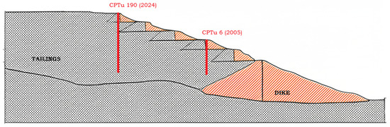
Figure 1.
Typical dam section.
Figure 1 presents a typical cross section of the dam, indicating the relative positions of two CPTu soundings, for example: CPTu 6 (2005), performed on the crest of a dike, and CPTu 190 (2024), executed farther into the reservoir, within the tailings deposit. Between 2005 and 2022, the dam underwent three upstream raises, resulting in an elevation gain of approximately 8 m. These construction stages significantly altered the internal stress distribution and hydrogeological conditions of the tailings mass. The underlying layers experienced additional self-weight consolidation and increased effective stress due to the progressive placement of overburden. Simultaneously, the phreatic surface migrated away from the dikes.
Some CPTu soundings, particularly those located along the alignment of the retaining dikes, required pre-drilling through overconsolidated or mechanically reinforced surface layers to allow cone penetration. These pre-drilled sections were excluded from stratigraphic analysis to avoid bias introduced by altered stress histories or artificial boundaries.
3.2. Dataset Characterization
The dataset used in this study contains measurements of , , , and u () from CPTu tests conducted in an iron mining tailings dam in Brazil. In total, the dataset contains 12 different tests, with varying locations and dates of test execution. Figure 2 depicts the number of measurements for each variable in the different tests. The nomenclature used for tests is , where refers to the company’s identification for the test and is the date of test conduction (day–month–year).
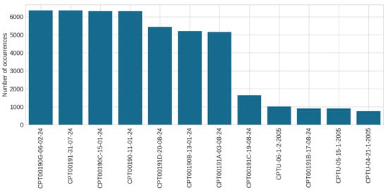
Figure 2.
Number of samples in each test.
As the distribution presented in Figure 2 shows, the majority of recent tests (year = 24) contain more samples than the older tests (year = 2005). This behavior is justified by two reasons: first, more recent test rely on modern equipment with superior resolution, i.e., while the modern equipment collected one sample at each centimeter, the older equipments collected one sample at each 2 cm; second, given the nature of mining tailing material disposal, the height of the dam increases with the time, implying in more depth. Table 2 summarizes the main statistical attributes for each test, including the maximum depth and the average values for each interest variable.
Table 2.
Statistical characteristics of each test, including number of samples, maximum depth in meters, and average values for , , and u in kPa.
To provide a clear understanding of variables’ distribution among the tests, we plot, in Figure 3, the probability distribution function (PDF) of depth (Figure 3a), (Figure 3b), (Figure 3c), and u (Figure 3d). The results show that most tests have similar behavior regarding u and depth, with distinctions occurring in and values. Also, one can note that changed severely among different locations in the site for the tests realized in 2024. Since sleeve friction reflects the interaction between the cone’s sleeve and the surrounding soil, it is highly influenced by physical properties of the material, such as grain size distribution, degree of saturation, and mineral composition. This spatial variability in highlights the importance of conducting analyses using data from closely spaced locations. Ignoring such heterogeneity may lead to misleading interpretations, particularly in applications such as the temporal monitoring of tailings deposition through clustering techniques.
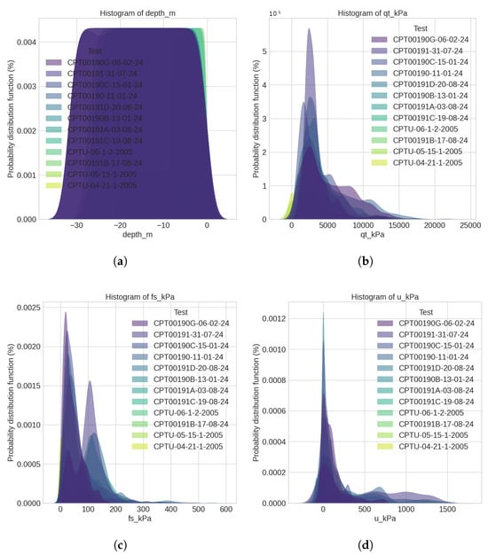
Figure 3.
Comparison of probability distribution function plots for interest variables among tests: (a) PDFs of depth; (b) PDFs of ; (c) PDFs of ; (d) PDFs of u.
3.3. Clustering-Based Stratigraphic Profile
This study proposes a four-step method, depicted in Figure 4, for generating soil stratigraphic profiles of tailing dams. In this section, we detail each step of the proposed method, including data preparation, model selection and tuning, clustering application, and stratigraphic analysis and validation.
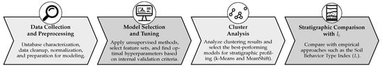
Figure 4.
Methodological workflow of the proposed approach, encompassing data preprocessing, unsupervised model selection and tuning, cluster-based analysis, and stratigraphic comparison via the Soil Behavior Type Index ().
Data preparation. The dataset obtained from field tests is error-prone, meaning that the values in the dataset may contain errors, be empty, or be outside the expected distribution. To mitigate the impact of such errors, we performed a preprocessing step to remove invalid entries (i.e., lines containing empty values and negative values of and ). For cases with higher positive values (i.e., distribution outliers), we did not conduct any treatment, as we understand they are not a result of measurement error. Additionally, since the dataset contains continuous values on different scales, we performed a scaling step to normalize each entry between 0 and 1, thereby increasing the clustering models’ potential to identify similarities [32].
Model selection and tuning. The second step in our proposed method aims to establish which model and respective configurations are the most suitable for soil stratigraphic profiling. For such purpose, we trained k-means, DBSCAN, MeanShift, and Affinity Propagation using all the points from the dataset and visually analyzed the generated clusters to verify whether groups have enough distinction. Then, for the model with the best results, we conducted a feature selection by analyzing different combinations of variables (i.e., , , and u), and we verified how each variable improved the clustering. Finally, we conducted a grid search for model refinement to define the best model’s attributes. For k-means, which uses the number of clusters as input, we applied the silhouette, elbow, and DBCV methods to find the best values [33,34].
Clustering application. After finding the clustering models with better results, the third step consists of applying the clustering algorithms and analyzing the distribution of groups across the different tests. In other words, this step intends to understand whether the realized clustering can provide meaningful results for the geomechanical profiling of soils. To reach such an objective, we plot the values of against the depth of measurement and vary the color according to the cluster number defined by the model. The reason for choosing is that such a metric exhibits less fluctuation in the PDF’s distribution (Figure 2) and because its value already includes u. Also, we analyze how clustering disposal varies with time by comparing profiles originating from closely spaced locations.
Stratigraphic analysis and validation. Finally, the last step of the proposed method consists of comparing the stratigraphic profile generated by clustering with the traditional approach based on . The main intention of this step is to verify if the clustering-based profile can support engineers in understanding the evolution of mining tailings disposal in the dam, and, for instance, offering insights regarding material behavior changes. It is important to highlight that the proposed approach is not intended to replace the traditional approach, but rather to offer additional support to decision makers of dam projects.
3.4. Implementation Details
We implemented the proposed clustering-based stratigraphic profile method using Python 3.11 scripts. The scripts are available in the repository https://codigos.ufsc.br/arthur.miguel/ml-stratigraphy, accessed on 31 July 2025. This study relies on the following libraries and modules to process data, implement algorithms, and generate visualizations:
- Pandas 2.2.3. This library contains an open-source data analysis and manipulation tool broadly used in machine learning projects. We rely on the Pandas library [35] for data management and processing.
- Scikit-learn 1.6.1. This library contains several algorithms used for machine learning purposes [36]. We used Scikit-learn version 1.6.1 to implement the clustering algorithms used in this research.
- matplotlib 3.10.3. This library contains a comprehensive set of tools for creating visualizations in Python [37]. We rely on Matplotlib to generate most of the visualizations presented in this paper, including the stratigraphic profiles.
During the tuning step, we conducted a parallelized grid search to accelerate the process of establishing hyperparameter valuers for each model. This search explored the domain of values presented in Table 3. We then assessed results provided by the models using the parameter values that yielded the best scores for the clustering analysis, considering the silhouette, elbow, and DBCV indices.
Table 3.
Grid of values used for unsupervised models’ tuning.
4. Results
This section presents the results of the proposed clustering method for generating the soil stratigraphic profile. First, we discuss the performance of the evaluated models in producing clustering. Then, we assess cluster evolution with time using tests from closer locations. Finally, we use values to analyze how the clustering approach’s stratigraphic profile can support the geotechnical behavior of the mining tailing dam.
4.1. Model Selection and Tuning
The first step for model selection and tuning is feature analysis. As discussed in Section 3.3, we employed an incremental approach to analyze the behavior of the resulting clusters for each model, using different combinations of the interest metrics. Using k-means as a baseline, the analysis indicated that the best input for the clustering models was the triple (depth, , u), excluding . Given the discrepancy observed in the PDFs of (Figure 3c), the models produced clusters with intersection among groups. Figure 5 exhibits the clustering results for distinct combinations of features using the complete set of data. The results show that the inclusion of feature (Figure 5a,b) for the clustering models implies multiple intersections among the points, which hinders the separation of soil layers; on the other hand, the k-means results without (Figure 5c) show a clear separation among clusters. It is essential to note that unsupervised learning approaches lack a well-established method for feature selection, relying instead on the expertise of analysts. Also, we always include the depth as a feature, as it is a mandatory variable for stratigraphic profiling.
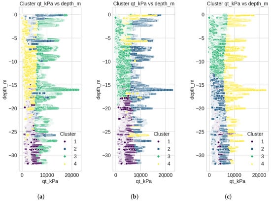
Figure 5.
versus depth and clustering results using distinct features in k-means training. (a) Model trained using 4-tuple (depth, , , and u). (b) Model trained using 3-tuple (depth, , and ). (c) Model trained using 3-tuple (depth, , and u).
The second step for model selection is evaluating how well each algorithm can separate the groupings. To assess the clustering performance of each algorithm, the methods were applied to CPTu190, a representative sounding selected for its recent execution and strategic location within the tailings reservoir. This profile captures a broad vertical sequence of the deposit, encompassing layers formed during distinct operational stages of dam raising. Its depth and stratigraphic diversity make it particularly suitable for evaluating the algorithms’ ability to distinguish meaningful geotechnical transitions associated with the dam’s construction history. Figure 6 presents the resulting stratigraphic segmentation produced by each method along the CPTu profile.
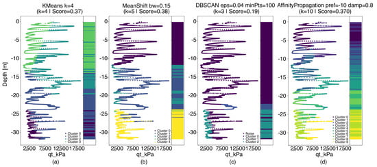
Figure 6.
Clustering result of soil stratigraphic profile for (a) k-means, (b) MeanShift, (c) DBSCAN, and (d) Affinity Propagation.
As depicted in Figure 6, the k-means and MeanShift methods showed similar clustering behavior and provided the most geotechnically consistent results. In both cases, the algorithms delineated four to five distinct layers that correspond well with known depositional and consolidation events. A near-surface layer, likely associated with recent tailings deposition, was separated from underlying strata. Intermediate zones of varying stiffness were also identified, including a deeper, more consolidated layer interpreted as part of the original foundation or early-stage tailings. These results demonstrate the capability of both methods to distinguish stratigraphic units with distinct geomechanical histories, making them more suitable for supporting geotechnical characterization in tailings dams.
The Affinity Propagation algorithm yielded many clusters, resulting in an overly fragmented profile. This over-segmentation hinders the identification of coherent stratigraphic layers or depositional patterns and limits the interpretability of operational history or material behavior over time. The excessive granularity captures local fluctuations in the CPTu parameters rather than meaningful transitions in geotechnical properties. In contrast, the DBSCAN algorithm produced a much coarser segmentation, with fewer and subtler divisions between clusters. Although the method successfully avoids arbitrary predefinition of the number of clusters, the resulting groupings did not align with expected stratigraphic transitions or reflect known stages of tailings deposition. This suggests that DBSCAN’s density-based criteria may be insufficiently sensitive to vertical variability in CPTu profiles, particularly when strong parameter discontinuities do not accompany distinct depositional events.
A wide range of validation indices is available in the literature for tuning unsupervised machine learning models [38]. Regarding k-means, the algorithm depends on initially defining the number of clusters. As discussed in Section 3.3, we rely on both the silhouetteand the elbow approaches for establishing such a value. Figure 7 depicts the silhouette and elbow charts. While the elbow chart (Figure 7b) suggests using four clusters, the silhouette chart (Figure 7a) indicates three clusters, given the larger increase from to than from to . However, upon further inception demonstrated to have higher cohesion and separation for the context of this application, this result was used for results and discussions. Also, the silhouette score with was higher than with . Similarly, since Affinity Propagation is highly sensitive to Euclidean distances, we used the silhouette index to tune its regularization parameters, resulting in preference and damping values of and , respectively. For DBSCAN and MeanShift, we employed the DBCV index, which is more appropriate for density-based clustering as it directly accounts for density rather than distance [34].
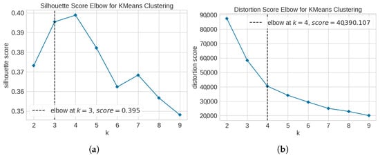
Figure 7.
Silhouette (a) and elbow (b) charts for determining number of clusters in k-means.
4.2. Stratigraphic Profile Through Clustering
To evaluate the temporal and spatial evolution of stratigraphic profiles within the tailings deposit, we selected two CPTu soundings conducted nearby but at different times: CPTU-06-1-2-2005 and CPT00190-11-01-24. The spatial positioning of these tests along the dam section is illustrated in Figure 1. CPTU-06 was performed in 2005, at the alignment of an upstream dike, whereas CPTu190 was executed in 2024, within the central portion of the tailings mass, further from the dike. This configuration allows for a comparative analysis of how the deposit has evolved over nearly two decades of operational changes and successive dam raisings.
Figure 8 presents the k-means clustering results applied to both profiles, alongside the measured cone resistance () as a function of depth. The clusters provide a basis for interpreting lithostratigraphic transitions and identifying layers potentially influenced by consolidation, new deposition, or changes in stress state over time.
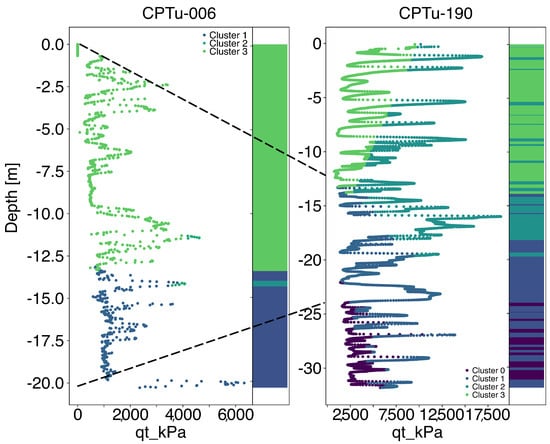
Figure 8.
Evolution of k-means clustering distribution in two tests from a closer location in a 19-year interval. The left side contains measurements from 2005, and the right side contains data from 2024. The dashed lines indicate the related soil layers after raising the mining tailings.
As the CPTU soundings were conducted at different times and during distinct stages of dam elevation, as shown in Figure 1, two dashed lines were added to Figure 8 to approximately indicate the relative position of the 2005 profile within the 2024 sounding. These reference lines account for the estimated thickness of the tailings layers deposited during the latest upstream raising stages. A comparative analysis reveals a strong correspondence between the clusters identified in each profile, particularly when aligned by equivalent depths relative to the dam’s original elevation.
Two main observations arise from the analysis of the stratigraphic profiles depicted in Figure 8. First, raising mining tailings in the 19-year interval implied adding a specific pattern (represented by cluster 0), such that a cluster appears in soil layers below 25 m depth. Second, during the interval between the measurements, 8 m of mining tailing material was disposed of in the dam, such that a continuous raising implied a compression of the material, which is reflected by the emergence of cluster 2, with . This suggests that the stratigraphic patterns delineated by the k-means algorithm are consistent and capable of capturing meaningful transitions within the tailings mass, despite the temporal and spatial differences in the data acquisition campaigns.
Figure 9 depicts the clustering results obtained through the MeanShift model. The model provided results similar to k-means. The main difference occurred in the CPTu-190 test, in which most clustering occurred by layers of depth, with few intersections between 8 and 25 m of depth, corresponding to the soil measured in the CPTu-006. Regarding the geomechanical aspects, such a result is consistent with the compression of mining tailings occurring with the dam elevation. Such a result suggests that both models, k-means and MeanShift, are complementary for stratigraphic profiling.
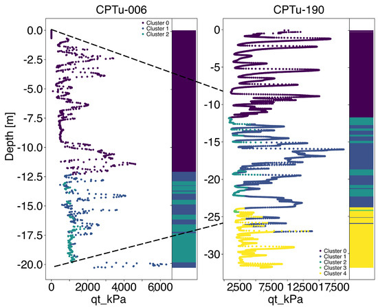
Figure 9.
Evolution of MeanShift clustering distribution in two tests from a closer location in a 19-year interval. The left side contains measurements from 2005, and the right side contains data from 2024. The dashed lines indicate the related soil layers after raising the mining tailings.
4.3. Stratigraphic Profile Based on Soil Behavior Index ()
To complement the cluster-based stratigraphic interpretation, we analyzed the variation of the Soil Behavior Type Index () along depth for the two CPTu soundings selected: CPTu-06 (executed in 2005) and CPTu-190 (executed in 2024). Figure 10a,b display the distribution of for each test individually, while Figure 10c presents the combined profiles. In this composite view, the depth profile of CPTu-06 was corrected to account for the approximate vertical offset introduced by the dam raises, allowing alignment with the corresponding elevation in the 2024 profile.
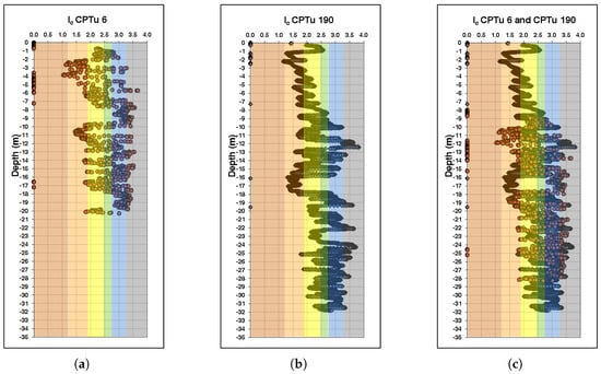
Figure 10.
versus depth. (a) CPTu 6; (b) CPTu 190; (c) CPTu 6 and CPTu 190. Colored bands represent the intervals and corresponding soil behavior types described in Table 1.
The results reveal that values span a wide range across the profiles, covering multiple soil behavior types—from clean sands and silty sands to clayey materials—as defined by the classification boundaries in Table 1. This variation highlights the heterogeneity of the deposit, which is expected in upstream-raised tailings dams due to their operationally driven deposition processes. Despite this variability, the comparative analysis of the aligned profiles shows strong consistency in the behavior of corresponding layers between the two tests. In particular, layers identified in 2005 exhibit similar values to those found at the adjusted depths of the 2024 profile. This reinforces the interpretation that the material remains compositionally similar across time, even though local variations in stress history and deposition conditions influence the values via their dependence on , , and (Equation (1)).
The stratigraphic profile generated from the index reflects a heterogeneous behavioral response of the tailings material, capturing transitions between different soil behavior types even within a single depositional unit. Notably, this heterogeneity is consistent across time, as evidenced by the similarity of values in corresponding layers from both the 2005 and 2024 CPTu tests. When analyzed jointly with the stratification derived from clustering methods, the profile provides a more comprehensive view of the material’s history. While the index classifies soil behavior based on mechanical response, clustering algorithms—especially those incorporating spatial and statistical data patterns—can distinguish differences within the same material class. These differences are often indicative of the depositional sequence and the consolidation history of the tailings, which are crucial for understanding mechanical evolution. This integrated approach offers a valuable perspective for geomechanical modeling and stability assessment of tailings dams, as it highlights behavioral shifts that may not be captured through traditional classification schemes alone.
5. Discussion
The results of this research study indicate that unsupervised machine learning methods can substantially improve the stratigraphic interpretation of CPTu data in mining tailings deposits. Such a result follows the findings from the literature [27,28] that, despite the clustering method, demonstrate the benefit of unsupervised learning for the enrichment of stratigraphic profiles. Among the clustering methods evaluated, k-means and MeanShift demonstrated superior performance in delineating geotechnically meaningful strata. Their stratigraphic outputs aligned with known depositional and consolidation histories, showing consistency across temporally distinct CPTu profiles.
Although k-means was effective, its main limitation lies in predefining the number of clusters (k), which introduces subjectivity and requires expert calibration. MeanShift, while capable of identifying clusters without predefined k, was sensitive to kernel bandwidth selection, and its performance degraded in regions of varying data density. Affinity Propagation and DBSCAN presented challenges: the former tended to over-segment the data into excessive clusters, the latter often failed to detect stratigraphic boundaries in the presence of subtle density changes. This result partially confirms the findings of previous studies [27,31], indicating that, once adjusted, k-means delivers promising results for stratigraphic profile analysis. The use of MeanShift is novel, as the method has not been previously investigated. On the other hand, previous studies have demonstrated promising results in developing stratigraphic profiles with DBSCAN [28], which our results do not confirm.
Another key finding of this study is the added value of combining clustering-based profiles with traditional stratification. While provides a standardized soil behavior classification, it often overlooks behavioral transitions caused by operational variability or consolidation. Clustering, by contrast, can detect shifts within the same material class, offering insights into the depositional history and mechanical evolution of the deposit. This integrative perspective enhances geotechnical modeling in stability assessment, liquefaction risk zoning, and dam raise planning.
Even with the discussed advantages of leveraging clustering for stratigraphic profiling of soils, we understand that the conducted study has limitations that analysts should consider carefully:
- Model tuning and selection depend on data quality and expertise. In the second step of the conducted method (Figure 4), we removed the variable from the input values of the models, a decision based on the analysis of clustering results generated by the k-means algorithm. As unsupervised learning methods lack an objective approach for feature selection, such decisions depend on the expertise of analysts in interpreting the graphical results, which is subjective.
- The generated stratigraphic profiles reflect the behavior of the specific dam. The set of clusters generated depends on the data used for model training; consequently, it is not possible to infer that a similar behavior will appear in other dams. Thus, reproductions of this study must consider an entire execution of the proposed workflow (Figure 4).
- Pore pressure values reflect conditions at the time of testing, without accounting for seasonal fluctuations or drainage effects during deposition. As long-term hydrogeological monitoring data were not available, measurements were incorporated as instantaneous values, which may limit the interpretation of hydro-mechanical behavior and its temporal variability. Additionally, the analysis did not include a correlation between the identified clusters and specific operational practices (e.g., discharge rate or particle size segregation) during dam construction, as detailed historical operational records were unavailable.
- Lack of validation through laboratory tests to confirm the detected stratigraphic transitions. Ideally, one should validate the clustering results through tension evaluation of undisturbed samples collected simultaneously with the raising of the tailing dam. However, the mining company has not conducted such a test in the past, and given the large area of the tailing dam and the depth of the samples, collecting undisturbed samples is impractical nowadays.
- k-means and MeanShift exhibit intrinsic algorithmic constraints. k-means assumes Euclidean distance and user-defined k, favoring compact, spherical clusters, which may split or merge transitional zones with gradual – shifts; MeanShift eliminates the need for k, but its results are highly sensitive to kernel bandwidth—large bandwidths merge thin depositional veneers, whereas small ones fragment noise into spurious units.
6. Conclusions
This study demonstrated the applicability and benefits of machine learning techniques—specifically clustering algorithms—for enhancing the stratigraphic analysis of CPTu data in iron tailings dams. By comparing four clustering algorithms across 12 CPTu soundings from different operational stages, we identified that
- k-means and MeanShift were the most effective methods for detecting geotechnically significant stratigraphic layers;
- DBSCAN and Affinity Propagation showed limitations in dealing with vertical CPTu data, resulting in either under- or over-segmentation;
- The index, although widely used, may overlook internal variations linked to depositional history or consolidation, which clustering methods can identify;
- When aligned by depth and construction phase, clustered profiles from temporally distinct tests revealed consistent stratigraphic patterns.
Notably, the combined use of the Soil Behavior Type Index () and unsupervised clustering provides a robust and complementary framework for interpreting the mechanical and depositional evolution of tailings dams. While offers a standardized classification based on soil behavior, clustering enhances the detection of subtle transitions within similar material types, revealing operational and stratigraphic changes over time. This integrated approach represents a valuable tool for evaluating dam performance, conducting forensic interpretations, and developing more robust geomechanical models. Future studies should expand on spatial analysis and methods to 3D interpolation.
Author Contributions
Conceptualization, H.P.N. and R.J.P.; methodology, H.P.N., A.M.P.G. and R.J.P.; software, A.M.P.G. and R.J.P.; validation, H.P.N., R.P., M.B. and E.O.; investigation, R.P., M.B. and E.O.; resources, R.P., M.B. and E.O.; data curation, R.J.P.; writing—original draft preparation, H.P.N.; writing—review and editing, H.P.N. and R.J.P. All authors have read and agreed to the published version of the manuscript.
Funding
This research received no external funding.
Data Availability Statement
The data presented in this study are available on request from the corresponding author due to company commercial constraints.
Acknowledgments
The authors would like to thank Vale S.A. for providing the field data used in this study. We also acknowledge the PPGESE, PPGEC, and UFSC for the institutional support and data analysis. During the preparation of this manuscript, the authors used ChatGPT version 4o for the purpose of english review. The authors have reviewed and edited the output and take full responsibility for the content of this publication. This study was financed in part by the Coordenação de Aperfeiçoamento de Pessoal de Nível Superior–Brasil (CAPES)–Finance Code 001.
Conflicts of Interest
Authors Rafael Piton, Ezequias Oliveira, and Marieli Biondo are employed by the company Vale S.A. The remaining authors declare that the research was conducted in the absence of any commercial or financial relationships that could be construed as a potential conflict of interest.
Abbreviations
The following abbreviations are used in this manuscript:
| CPTu | Cone Penetration Tests with pore pressure measurements |
| DBCV | Density-Based Clustering Validation |
| Soil Behavior Type Index | |
| DBSCAN | Density-Based Spatial Clustering of Applications with Noise |
| PCA | Principal Component Analysis |
| Probability Distribution Function |
References
- Lune, T.; Powell, J.; Robertson, P. Cone Penetration Testing in Geotechnical Practice, 1st ed.; CRC Press: London, UK, 1997. [Google Scholar] [CrossRef]
- White, D. CPT equipment: Recent advances and future perspectives. In Cone Penetration Testing 2022; CRC Press: Boca Raton, FL, USA, 2022; pp. 66–80. [Google Scholar] [CrossRef]
- Adamo, N.; Al-Ansari, N.; Sissakian, V.; Laue, J.; Knutsson, S. Dam safety: The question of tailings dams. J. Earth Sci. Geotech. Eng. 2020, 11, 1–26. [Google Scholar] [CrossRef] [PubMed]
- Robertson, P. Soil classification using the cone penetration test. Can. Geotech. J. 1990, 27, 151–158. [Google Scholar] [CrossRef]
- Ekeanyanwu, C.V.; Obisakin, I.F.; Aduwenye, P.; Dede-Bamfo, N. Merging GIS and machine learning techniques: A paper review. J. Geosci. Environ. Prot. 2022, 10, 61–83. [Google Scholar] [CrossRef]
- Haghshenas, S.S.; Haghshenas, S.S.; Geem, Z.W.; Kim, T.H.; Mikaeil, R.; Pugliese, L.; Troncone, A. Application of harmony search algorithm to slope stability analysis. Land 2021, 10, 1250. [Google Scholar] [CrossRef]
- Zhou, B.; Li, C.; Andrade, J.E. Autonomous particle-shape-based classification and identification of calcareous soils through machine learning. Geotechnique 2024, in press. [Google Scholar] [CrossRef]
- Nierwinski, H.P.; Pfitscher, R.J.; Barra, B.S.; Menegaz, T.; Odebrecht, E. A practical approach for soil unit weight estimation using artificial neural networks. J. S. Am. Earth Sci. 2023, 131, 104648. [Google Scholar] [CrossRef]
- Vick, S. Planning, Design, and Analysis of Tailings Dams; BiTech: Richmond, BC, Canada, 1990. [Google Scholar]
- Chropeňová, D.; Slávik, I. Raising of Embankment of an Ore Tailings Pond and an Analysis of its Stability. Slovak J. Civ. Eng. 2023, 31, 24–33. [Google Scholar] [CrossRef]
- Lyu, Z.; Chai, J.; Xu, Z.; Qin, Y.; Cao, J. A Comprehensive Review on Reasons for Tailings Dam Failures Based on Case History. Adv. Civ. Eng. 2019, 2019, 4159306. [Google Scholar] [CrossRef]
- Robertson, P.K.; Melo, L.; Williams, D.J.; Wilson, G.W.; Report of the Expert Panel on the Technical Causes of the Failure of Feijão Dam I. Technical Report. B1 Technical Investigation Panel. 2019. Available online: https://bdrb1investigationstacc.z15.web.core.windows.net/assets/Feijao-Dam-I-Expert-Panel-Report-ENG.pdf (accessed on 31 July 2025).
- Liu, L.L.; Wang, Y. Quantification of stratigraphic boundary uncertainty from limited boreholes and its effect on slope stability analysis. Eng. Geol. 2022, 306, 106770. [Google Scholar] [CrossRef]
- Jewell, R.J.R.J.; Fourie, A.B. Paste and Thickened Tailings: A Guide, 3rd ed.; Jewell, R.J., Fourie, A.B., Eds.; Australian Centre for Geomechanics, University of Western Australia: Nedlands, Australia, 2015. [Google Scholar]
- Wroth, C.P. The interpretation of in situ soil tests. Géotechnique 1984, 34, 449–489. [Google Scholar] [CrossRef]
- Ezugwu, A.E.; Ikotun, A.M.; Oyelade, O.O.; Abualigah, L.; Agushaka, J.O.; Eke, C.I.; Akinyelu, A.A. A comprehensive survey of clustering algorithms: State-of-the-art machine learning applications, taxonomy, challenges, and future research prospects. Eng. Appl. Artif. Intell. 2022, 110, 104743. [Google Scholar] [CrossRef]
- Nazareth, A.F.D.V.; Lana, M.S. A methodology for the definition of geotechnical mine sectors based on multivariate cluster analysis. Geotech. Geol. Eng. 2021, 39, 4405–4426. [Google Scholar] [CrossRef]
- Frey, B.J.; Dueck, D. Clustering by passing messages between data points. Science 2007, 315, 972–976. [Google Scholar] [CrossRef]
- Min, E.; Guo, X.; Liu, Q.; Zhang, G.; Cui, J.; Long, J. A survey of clustering with deep learning: From the perspective of network architecture. IEEE Access 2018, 6, 39501–39514. [Google Scholar] [CrossRef]
- MacQueen, J. Some methods for classification and analysis of multivariate observations. In Proceedings of the 5th Berkeley Symposium on Mathematical Statistics and Probability, Statistical Laboratory, University of California, 21 June–18 July 1965 and 27 December 1965–7 January 1966; University of California Press: Oakland, CA, USA, 1967; pp. 281–298. [Google Scholar]
- Celebi, M.E.; Kingravi, H.A.; Vela, P.A. A comparative study of efficient initialization methods for the k-means clustering algorithm. Expert Syst. Appl. 2013, 40, 200–210. [Google Scholar] [CrossRef]
- Ester, M.; Kriegel, H.P.; Sander, J.; Xu, X. A density-based algorithm for discovering clusters in large spatial databases with noise. In Proceedings of the Second International Conference on Knowledge Discovery and Data Mining, Portland OR, USA, 2–4 August 1996; Volume 96, pp. 226–231. [Google Scholar]
- Schubert, E.; Sander, J.; Ester, M.; Kriegel, H.P.; Xu, X. DBSCAN revisited, revisited: Why and how you should (still) use DBSCAN. ACM Trans. Database Syst. 2017, 42, 1–21. [Google Scholar] [CrossRef]
- Comaniciu, D.; Meer, P. Mean shift: A robust approach toward feature space analysis. IEEE Trans. Pattern Anal. Mach. Intell. 2002, 24, 603–619. [Google Scholar] [CrossRef]
- Cheng, Y. Mean shift, mode seeking, and clustering. IEEE Trans. Pattern Anal. Mach. Intell. 1995, 17, 790–799. [Google Scholar] [CrossRef]
- Wang, K.; Zhang, J.; Li, D.; Zhang, X.; Guo, T. Adaptive affinity propagation clustering. arXiv 2008, arXiv:0805.1096. [Google Scholar] [CrossRef]
- San Roman Iturbide, O.; Botero Jaramillo, E. Identification of geotechnical units in soil exploration through principal component analysis and clustering. Int. J. Numer. Anal. Methods Geomech. 2024, 48, 1681–1699. [Google Scholar] [CrossRef]
- Sottile, M.G.; Crocker, J.A.; Roldan, L. Interpretation of CPTu data using machine learning techniques to develop the ground model of a dam. In Proceedings of the 7th International Conference on Geotechnical and Geophysical Site Characterization (ISC 24), Barcelona, Spain, 18–21 June 2024. [Google Scholar] [CrossRef]
- Cho, S.; Cho, B.; Kang, S.; Kim, H. Development of locally specified soil stratification method with CPT data based on machine learning techniques. In Proceedings of the Geotechnics for Sustainable Infrastructure Development, Hanoi, Vietnam, 28–29 November 2019; Springer: Singapore, 2020; pp. 1287–1294. [Google Scholar] [CrossRef]
- Shi, C.; Wang, Y. Nonparametric and data-driven interpolation of subsurface soil stratigraphy from limited data using multiple point statistics. Can. Geotech. J. 2021, 58, 261–280. [Google Scholar] [CrossRef]
- Nierwinski, H.P.; Custodio, L.A.; Barbosa, A.S.; Pfitscher, R.J. Use of Artificial Intelligence to Obtain a StratiGraphic Profile of Tailings Dams from CPTu Tests. In Geo-EnvironMeet 2025; ASCE Library: Reston, VA, USA, 2025; pp. 315–323. [Google Scholar] [CrossRef]
- Dauda, U.; Ismail, B. A study of normalization approach on K-means clustering algorithm. Int. J. Appl. Math. Stat 2013, 45, 439–446. [Google Scholar]
- Abdulnassar, A.; Nair, L.R. A Comprehensive Study on the Importance of the Elbow and the Silhouette Metrics in Cluster Count Prediction for Partition Cluster Models. Rev.-Geintec-Gest. Inov. Tecnol. 2021, 11, 3792–3806. [Google Scholar] [CrossRef]
- Moulavi, D.; Jaskowiak, P.A.; Campello, R.J.; Zimek, A.; Sander, J. Density-based clustering validation. In Proceedings of the 2014 SIAM International Conference on Data Mining, Philadelphia, PA, USA, 24–26 April 2014; SIAM: Philadelphia, PA, USA, 2014; pp. 839–847. [Google Scholar] [CrossRef]
- McKinney, W. Data Structures for Statistical Computing in Python. In Proceedings of the 9th Python in Science Conference, Austin, TX, USA, 28 June–3 July 2010; pp. 56–61. [Google Scholar] [CrossRef]
- Pedregosa, F.; Varoquaux, G.; Gramfort, A.; Michel, V.; Thirion, B.; Grisel, O.; Blondel, M.; Prettenhofer, P.; Weiss, R.; Dubourg, V.; et al. Scikit-learn: Machine Learning in Python. J. Mach. Learn. Res. 2011, 12, 2825–2830. [Google Scholar]
- Hunter, J.D. Matplotlib: A 2D graphics environment. Comput. Sci. Eng. 2007, 9, 90–95. [Google Scholar] [CrossRef]
- Vendramin, L.; Campello, R.J.; Hruschka, E.R. Relative clustering validity criteria: A comparative overview. Stat. Anal. Data Mining Asa Data Sci. J. 2010, 3, 209–235. [Google Scholar] [CrossRef]
Disclaimer/Publisher’s Note: The statements, opinions and data contained in all publications are solely those of the individual author(s) and contributor(s) and not of MDPI and/or the editor(s). MDPI and/or the editor(s) disclaim responsibility for any injury to people or property resulting from any ideas, methods, instructions or products referred to in the content. |
© 2025 by the authors. Licensee MDPI, Basel, Switzerland. This article is an open access article distributed under the terms and conditions of the Creative Commons Attribution (CC BY) license (https://creativecommons.org/licenses/by/4.0/).