Incremental Capacity and Voltammetry of Batteries, and Implications for Electrochemical Impedance Spectroscopy

Abstract

Incremental capacity analysis (ICA), where incremental charge (Q) movements associated with changes in potential are tracked, and cyclic voltammetry (CV), where current response to a linear voltage sweep is recorded, are used to investigate the properties of electrochemical systems. Electrochemical impedance spectroscopy (EIS), on the other hand, is a powerful, non-destructive technique that can be used to determine small-signal AC impedance over a wide frequency range. It is frequently used to design battery equivalent-circuit models. This manuscript explores the relationships between ICA, CV and EIS and demonstrates how sweep rate in CV is related to charging (C) rate in ICA. In addition, it shows the connection between observations linked to rate of charge movement in CV and ICA and intermittent, irregular behavior seen in EIS when performed on a battery. It also explains the use of an additional DC stimulus during EIS to ensure reliability of battery impedance data and to facilitate equivalent-circuit modeling, and suggests a method for obtaining data analogous to CV from a whole battery without risking its destruction.

1. Introduction

Cyclic voltammetry (CV) and incremental capacity analysis (ICA), both of which relate aspects of electrochemical activity to cell terminal voltage, are widely used in the evaluation of electrochemical systems. CV measures current while potential is swept linearly as a function of time [1,2,3,4,5], whereas ICA tracks charge (Q) movements associated with changes in potential ($dQ/dV$) when a constant current is applied [6,7]. More specifically, incremental capacity refers to changes in increments of charge $\delta Q$ seen with successive fixed increments of voltage $\delta V$[7]. An incremental capacity curve is constructed by tracking the increments of capacity associated with the voltage steps. Differential voltage analysis (DVA) on the other hand plots the reciprocal relationship $dV/dQ$ [8] Both ICA and DVA (which will not be discussed further in this manuscript) describe cell phase transition characteristics during intercalation and de-intercalation processes at the electrodes during charging and discharging [9], but constitute different ways of viewing this information.

While these methods provide simple but useful information about peak currents and potentials that can help to characterize the electrochemistry of a system, a further method, electrochemical impedance spectroscopy (EIS), holds a special place because it presents data as a function of frequency that can reveal a great deal of information about the characteristics and condition of a cell and inform the development of equivalent-circuit models (ECMs) [5,10,11,12]. Accompanying all these is the most basic method of charging and discharging a cell (cycling), which allows the investigator to produce plots of potential against some other variable (typically charge moved), the shapes of which are determined by a cell reaction’s thermodynamic and kinetic properties [5,12].

Although the above methods are usually viewed as distinct techniques that give the investigator different types of data, they are related both mathematically and in terms of the information they can provide. Very slow cycling experiments and EIS at extra-low frequencies (ELFs, down to as low as 1.0 μHz) that reflect the real-world usage cycles of rechargeable batteries [13,14,15,16] have led to observations enabling us to clarify connections between the above techniques, and to suggest a simple and inexpensive method for carrying out ICA on batteries. They also explain the recently reported need to use background direct currents to suppress electrochemical behavior that interferes with EIS measurements at ELFs [16].

Relationships between CV and ICA have been explored previously [5,12,17]. In this paper we extend these ideas with an emphasis on the significance of very low sweep or cycling rates, and discuss their relevance to EIS, particularly when carried out at ELFs, and the implications for fitting of battery ECMs. We suggest in addition how our method might be used to allow analyses analogous to CV to be carried out on intact lithium-ion batteries. Conventional CV involving the application of a voltage ramp with constant $dV/dt$ is potentially hazardous because of the risk of thermal runaway, leakage of electrolyte or even explosion as a result of the uncontrolled currents that might be generated. Other problems include the relatively small active electrode area in a lithium-ion cell, which could limit sensitivity and accuracy of CV, and potential unsuitability of the battery electrolyte for this procedure.

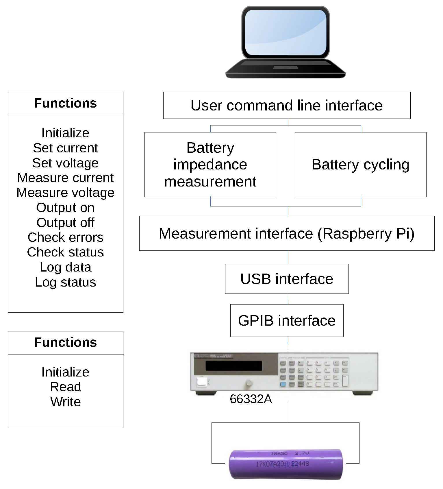
2. Experimental Methods

The battery used in the present experiments was a new lithium nickel cobalt aluminum oxide (NCA) 4.8 Ah 3.7 V 21700 cell. Measurements were taken at 22 °C using two-quadrant precision sources (HP/Agilent/Keysight 66332A units) via four-wire connections controlled through GPIB interfaces by Raspberry Pi 4 computers running custom software written in C [16,18] (Figure 1).

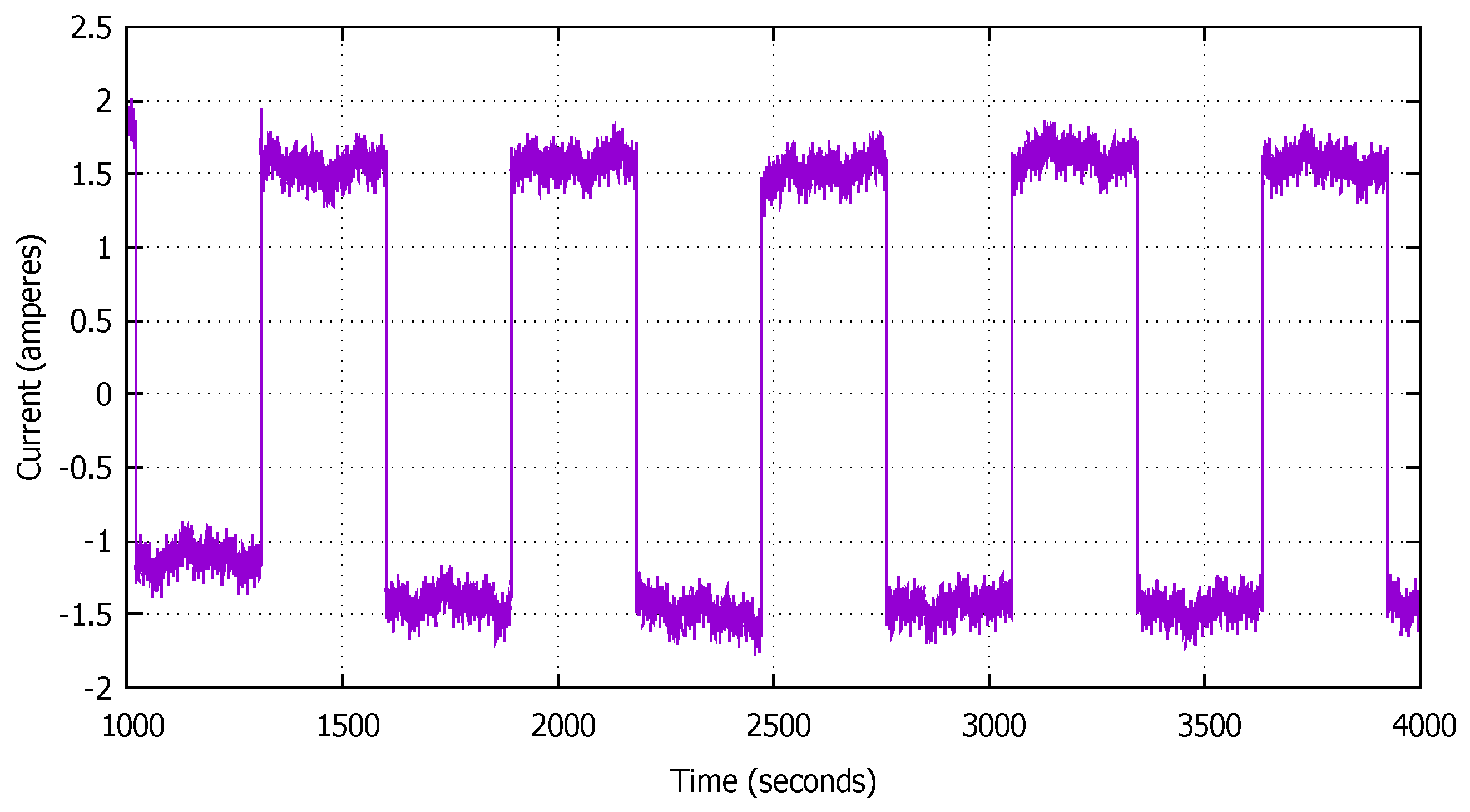
2.1. Battery Cycling and Incremental Capacity and Voltammetric Analysis

The software used for battery cycling, “bcp66”, is a command line program called by scripts that set parameters for each run, allowing many experiments to be queued and executed (see https://github.com/CDunnNZ/Batteries for source code, accessed on 21 May 2025). Typically batteries are cycled according to industry standard CC (constant current) or CC-CV (constant current-constant voltage) protocols. (The acronym “CV” is used in electrochemical research to designate cyclic voltammetry, but in an industrial battery context the same acronym is used to designate “constant voltage”, a part of charging and discharging protocols). The bcp66 program allows the user to specify charge and discharge currents (cycling rate calculated with reference to the cell’s nominal capacity in ampere-hours) which are applied in constant current mode until pre-specified voltage limits are reached. At this point, a constant voltage phase may begin if desired; if not, the software stays in constant current mode and switches immediately to the next charge or discharge phase. Rest periods can also be requested. The software allows the user to specify currents at which to end constant voltage phases, and dwell times, the maximum period to wait for constant voltage phases to end. Other parameters include number of cycles, the final charge (percent) at the end of cycling, and a wait time or period to continue recording after cycling is finished and current has returned to zero. Output is presented in a “.tvi” text file with time, voltage, current, charge moved ($\Delta$Q) and repetition-number columns. The 66332A units return approximately eight records per second.

2.1.1. Data Processing

Data were processed by scripts in MATLAB^® or AWK. All processing starts by importing timestamped current and voltage values from .tvi files created by the measurement system into arrays containing time, voltage and current data. An arbitrary voltage interval is specified (5 mV in the examples shown in this manuscript), and a calculation performed as the script loops through the arrays to calculate the quantity of charge moved and the time taken for each voltage increment. This information is then used to create three further arrays containing charge moved as a function of time, charge moved as a function of voltage (incremental capacity $dQ/dV$) and change in voltage as a function of time ($dV/dt$) for each voltage increment.

2.1.2. Connecting Incremental Capacity and Voltammetry

We assume a battery has some function relating open circuit terminal voltage to charge available, $V\left(Q\right)$. In the case of CV a linear voltage ramp is applied, so that

$${\displaystyle \frac{dV}{dt}}=k$$

(1)

hence

$$V\left(t\right)=kt+V_0$$

(2)

where k is the constant voltage sweep rate, t is time in seconds, and $V_0$ the battery’s open circuit voltage at the start of the sweep. Also

$$I\left(t\right)={\displaystyle \frac{dQ}{dt}}={\displaystyle \frac{dQ}{dV}}{\displaystyle \frac{dV}{dt}}=k{\displaystyle \frac{dQ}{dV}}$$

(3)

In CV, current $I\left(t\right)$ is plotted against voltage $V\left(t\right)$, and the rate of change of voltage ($dV/dt$) is constant. Current represents rate of reaction, which varies as the absolute voltage varies. Equation (3) shows that incremental capacity $dQ/dV$ is in fact equal to $I\left(t\right)/k$, which is current ($dQ/dt$, which may vary in this scenario) divided by the voltage sweep rate k, a constant ($dV/dt$, which does not vary) that now acts as a scaling factor.

Furthermore, CV experiments assume that the concentration of reagents is not affected by diffusion, which is equivalent to saying that the sweep rate k (i.e., $dV/dt$ held constant) is slow (so that concentration gradients that would build up by diffusion-affected processes do not form). Moreover, the peaks of a CV plot are influenced by sweep rate [1,3].

In ICA, a constant current is used, so

$$I\left(t\right)=c$$

(4)

and so

$$I\left(t\right)={\displaystyle \frac{dQ}{dt}}={\displaystyle \frac{dQ}{dV}}{\displaystyle \frac{dV}{dt}}=c$$

(5)

where c is the constant current value. Then

$${\displaystyle \frac{dQ}{dV}}={\displaystyle \frac{c}{\left[\frac{dV}{dt}\right]}}$$

(6)

and ${\displaystyle \frac{c}{\left[\frac{dV}{dt}\right]}}$ (which is equal to $dQ/dV$ as shown by Equation (6)) is plotted against voltage. Note the contrast between the CV scenario described by Equation (3), where $dV/dt$ is constant (k), and the ICA scenario of Equation (6) where current is held constant (c) and $dV/dt$ can vary.

Constant-current data can be used to generate plots that are representative of ICA or a current-derived analogy of CV (in which cell voltage is presented on the x-axis as an independent variable). The latter are not conventional electrochemical CV plots because we have not applied a voltage ramp and measured the current response. Rather, we have applied constant charge and discharge currents and tracked voltage increases and decreases with time at the sample rate of the instruments. When we plot the data, however, we do so in the same way as if voltage had been increased in a linear manner by the operator. In the interests of clarity, we will therefore refer to “CV-type” or “current-derived” plots in this manuscript.

It is worth noting here that the assumption that a battery obeys a state equation relating open-circuit terminal voltage to charge available, $V\left(Q\right)$, is not true in general. If we accept that the battery embodies a fractional (constant-phase) element (CPE), this is mathematically not the case. (In general, charge Q is a functional of voltage, $Q=Q\left[V\left(t\right)\right]$. Differentiating with respect to time yields

$$I\left(t\right)={\displaystyle \frac{dQ\left(t\right)}{dt}}={\int }_{t^{\prime }=-\infty }^t{\displaystyle \frac{\delta Q\left(t\right)}{\delta V\left(t^{\prime }\right)}}{\left.{\displaystyle \frac{dV}{dt}}\right|}_{t=t^{\prime }}d{t}^{\prime }$$

and this full form must be evaluated. In a typical quasi-static situation this is not necessary. Discussion of this is beyond the scope of this manuscript).

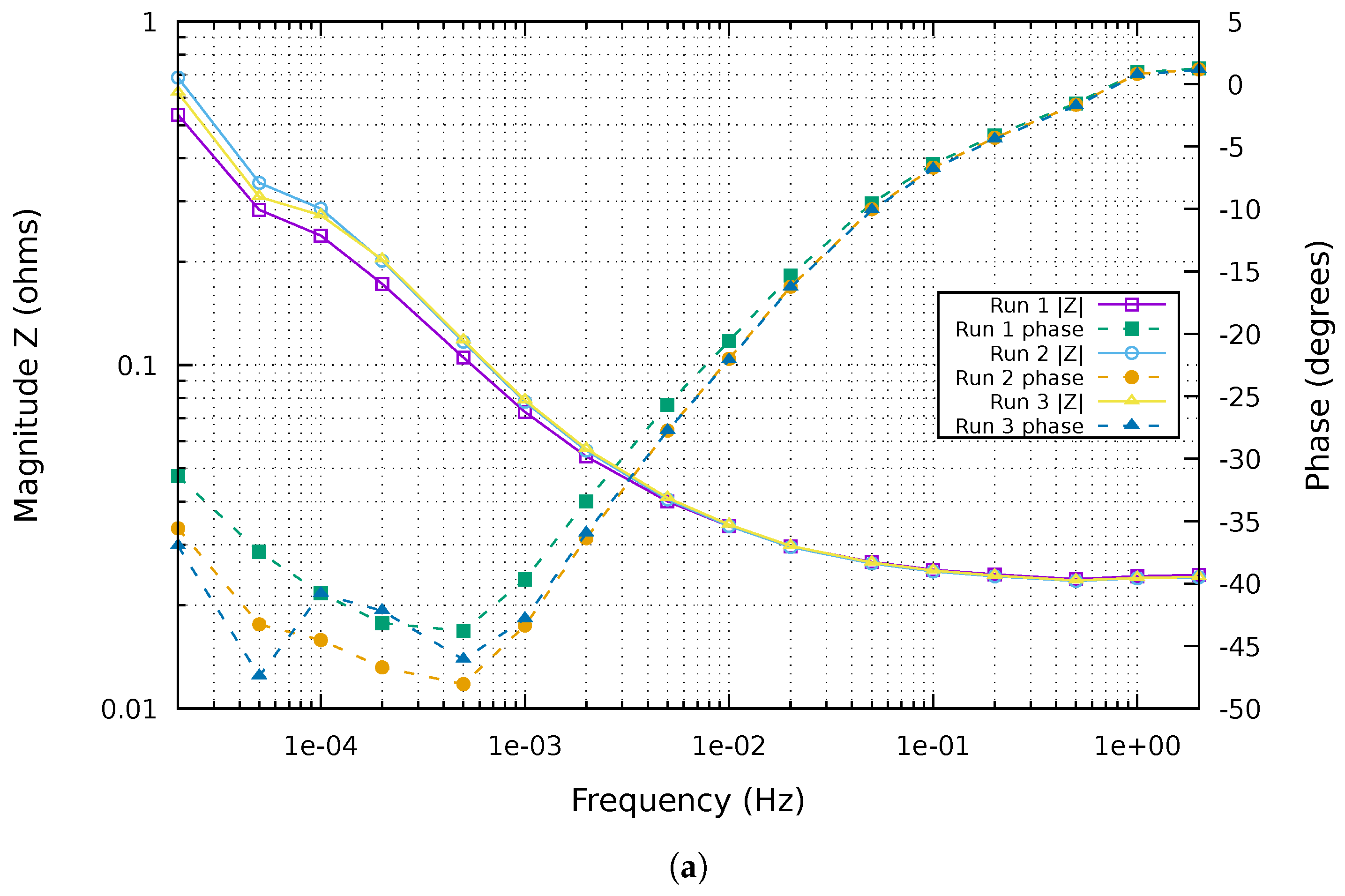
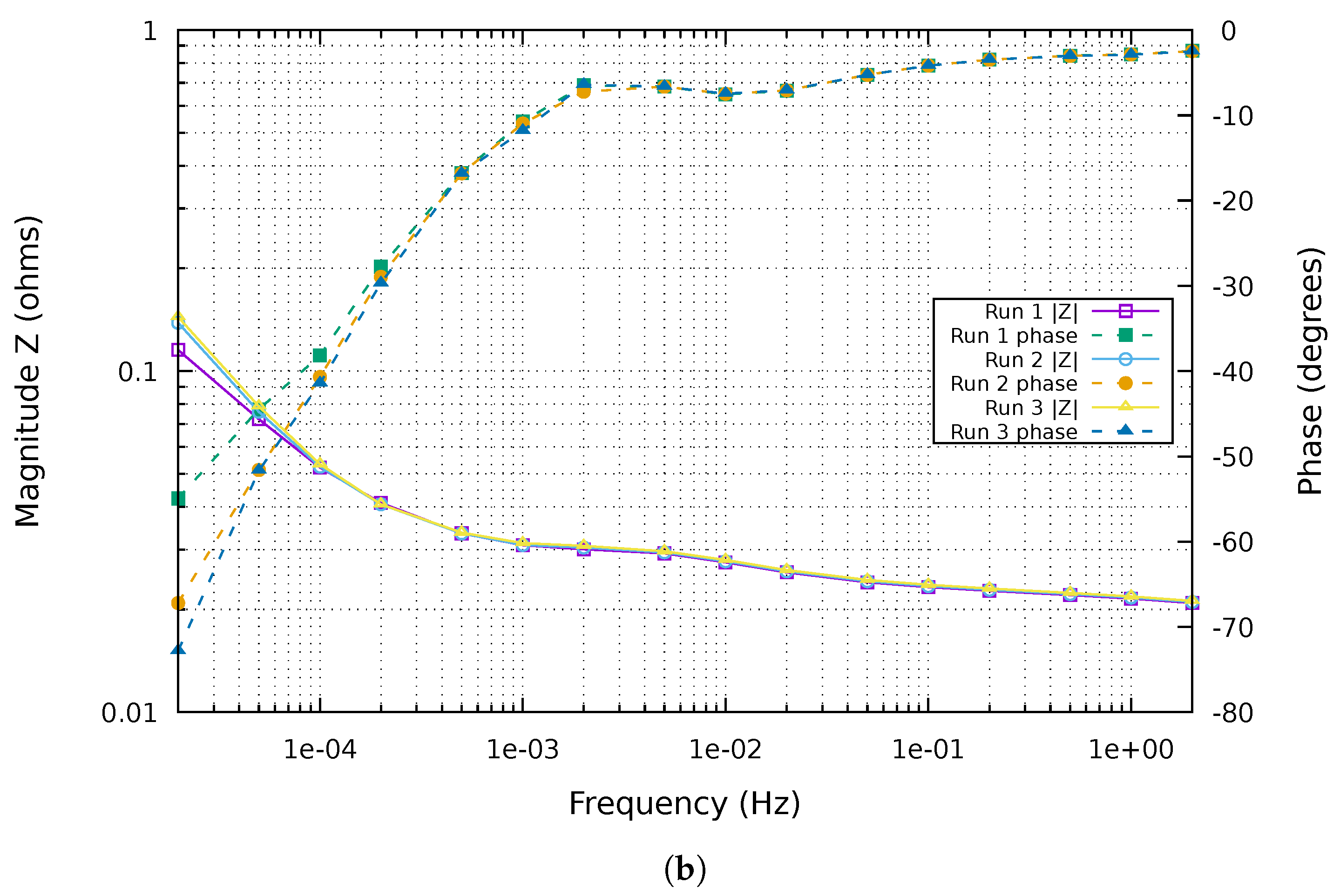
2.2. EIS Measurement

Full details of the procedure used to conduct EIS at ELFs using the 66332A units controlled by Raspberry Pi computers via GPIB interfaces have been reported previously [16]. Using the hardware described above, another command line program written in C, “bzdcp66” (see https://github.com/CDunnNZ/Batteries, accessed on 21 May 2025), is used to make multitone impedance measurements by sourcing and sinking current, and recording times, currents and voltages in three-column .tvi files. The complex impedance $Z\left(\omega \right)$ for each frequency of interest

$$Z\left(\omega \right)={\displaystyle \frac{\left|V\right|}{\left|I\right|}}{e}^{j({\varphi }_V-{\varphi }_I)}$$

(7)

is obtained from the .tvi data by performing a discrete-time Fourier transform using a program based on software originally designed for use with SPICE [19], and the magnitude and phase results presented in Bode plots (Nyquist plots convey no useful information at ELFs). The measurement software is distinguished by its ability to impose a small-signal, multiple-frequency (multitone) stimulus in addition to a “working” stimulus signal simultaneously. This is accomplished by superimposing the EIS multitone, which involves very small voltage perturbations and hence very small charge movements, on a periodic square wave which is associated with much greater movement of charge and aims to simulate the effect of a working DC signal (Figure 2).

As reported previously [16] and demonstrated by the example in Figure 3 (which is based on data from an early experiment with the apparatus described in Figure 1), this charge displacement stabilizes the impedance spectrum against impedance drift phenomena and maximizes measured data quality, showing the true working impedance of a battery and optimizing data for ECM fitting [16]. We suggest that there is a relationship between the effects of rate of charge movement on EIS impedance measurements and what we observe in ICA and CV-type plots derived from battery cycling experiments.

2.3. ECM Fitting

Electrochemists and engineers use ECMs to characterize a battery’s internal processes and to describe and predict state of charge and state of health. Since the publication of the work of Randles in 1947 [20], researchers have acknowledged the need to use CPEs, also known as fractional (or “lossy”) capacitors, in battery models [10]. This is because the double-layer capacitance of solid electrodes is not purely capacitative and displays frequency dispersion, and CPEs are necessary to model this non-ideally polarizable behavior [21].

The equation for the impedance of a CPE is

$$Z_{CPE}={\displaystyle \frac{1}{C_F{s}^{\alpha }}}\mathrm{for}\alpha \in (0,1)$$

(8)

where $C_F$ is the CPE value (its pseudo- or fractional capacitance, a constant with the dimensions $F{s}^{\alpha -1}$), $\alpha$ is the CPE fractional order exponent, $s=j2\pi f$ (where $2\pi f=\omega$, the angular frequency), and f is the frequency in hertz [22]. The total impedance of an R-CPE model is expressed as

$$\begin{array}{cc}\hfill Z_{R-CPE}& =R_s+Z_{CPE}\hfill \\ \hfill & =R_s+{\displaystyle \frac{1}{C_F{s}^{\alpha }}}\hfill \end{array}$$

(9)

where $R_s$ is the series resistance and $Z_{CPE}$ is the impedance of the CPE (Equation (8)) in ohms.

$Z_{CPE}$ has a constant phase angle at $\alpha \pi /2$ [23], whereas the phase shift in pure capacitors (where $\alpha =1$) is $\pi /2$. $\alpha$ is related to the deviation of the straight capacitative line from 90 degrees by angle $90(1-\alpha )$ degrees [21].

Conventional EIS and ECM fitting involves the presentation of data in the form of Nyquist plots in which the changing relationship between real and imaginary impedance with varying frequency reveals patterns characteristic of distinct electrochemical processes [24]. This information is used to generate ECMs in which an individual circuit element is used to represent each of these processes. Such ECMs can become complicated, with many elements being required to model the cell’s behavior [10,24,25].

We have found that a three-element ECM models real-world measured battery impedance data with precision similar to individual sample error [11]. The formulation of such an ECM is made possible by the EIS measurement technique at ELFs as described in Section 2.2 [16]. The fitting procedure used has been described previously [11], and involves generation of an ECM via an optimization method based on the downhill simplex algorithm of Nelder and Mead [26] that is implemented in C as a command line program [27]. The optimization target is defined as a root mean square error (RMSE) value calculated from complex impedances as indicated by the available data. The final RMSE reflects how well the model fits the data, with a perfect fit defined as an RMSE approaching zero, while higher values indicate noisier, poorer quality or ambiguous data. As previously [16], modeling starts with the simplest ECM, a single resistor and CPE in series (R-CPE). If the RMSE indicates a poor fit, we move to the next model in the chain of complexity, a resistor and two CPEs in series (R-CPE-CPE). Links between these observations and electrochemical behavior suggested by cycling experiments (Section 2.1) are explored.

3. Results and Discussion

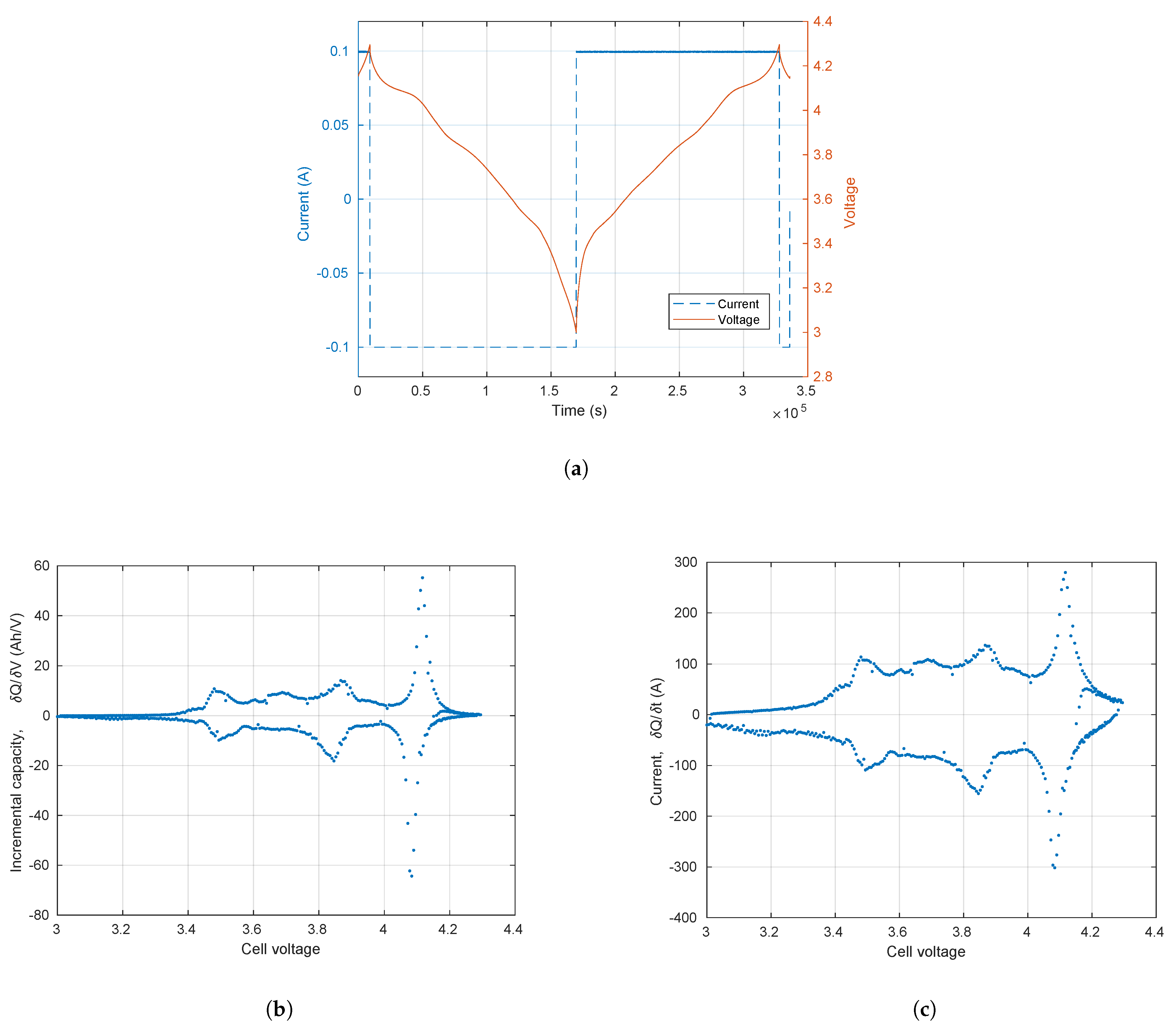
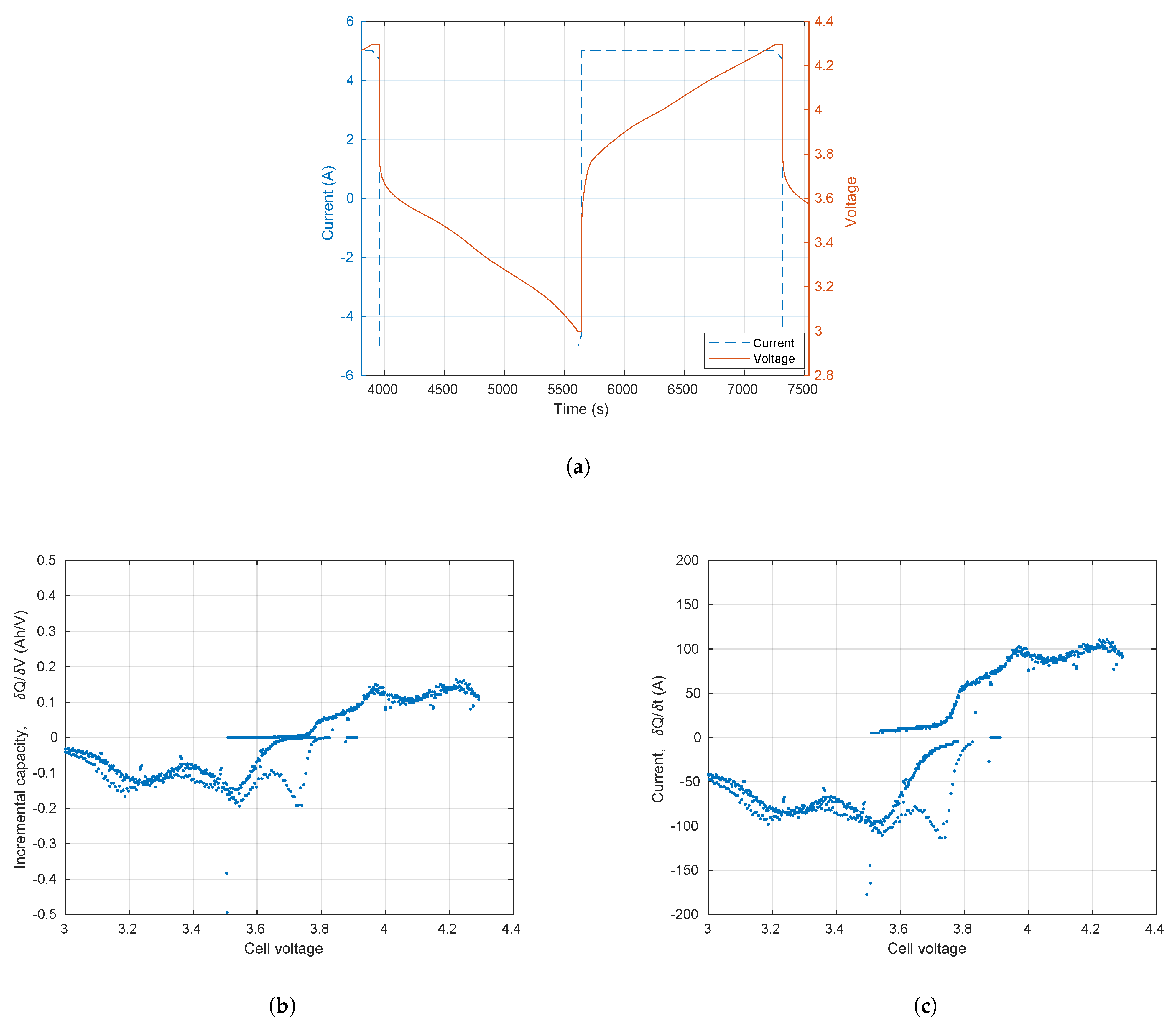
3.1. Incremental Capacity and Voltammetry

Figure 4a shows a complete slow (C/48) discharge-charge cycle with its voltage response. Note the uneven voltage trace: this is characteristic of slow charging and discharging and corresponds to changes in the potential required to move charge. Plateaus in the voltage versus time curve correspond to peaks in the $dQ/dV$ (ICA) plot in Figure 4b (shown most prominently by the shallow tangent and large peak at approximately 4.1 V). Each peak represents a different chemical reaction or intercalation environment, and the area under the peak shows the capacity of that process. Thus, voltage plateaus (shallow tangents) in Figure 4a represent large capacity increments in Figure 4b (i.e., a lot of charge is moved for a small voltage change). These peaks describe cell phase transition characteristics during the intercalation and de-intercalation of lithium ions [9]. Changes in peak position and size have been investigated as potential markers of battery aging, with the literature tending to focus on LiFePO₄ cells [6,7,28,29,30], although data on NCA [31] and other chemistries [32,33,34,35] are also available.

We see the same pattern of peaks when charge movement is related to increments of time and presented as current in a CV-type plot (Figure 4c). This is because $dQ/dt$ (i.e., current, as conventionally plotted in CV), is in fact $dQ/dV$ (i.e., incremental capacity) multiplied by the scaling factor k (Equation (3)). Moreover, ICA is $dQ/dt$ (which we define as c; Equation (5)) multiplied by $1/k$ (i.e., ${\displaystyle \frac{1}{dV/dt}}$; Equation (6)). Although we have not carried out a true CV on the battery for reasons discussed earlier (Section 2.1.2), these relationships and observations indicate that CV might yield the same information as ICA in the presence of very low rates of movement of charge.

Figure 5a shows the effect of increasing the rate of charge/discharge from 100 mA (C/48) to 5 A (approximately 1C): the voltage response to the charge/discharge current becomes smoother, reflecting increased uniformity of charge movement across the cell’s terminal voltage range. The initial slope $dV/dt$ on switching from discharge to charge is vertical because there is a large change in potential difference over the resistive component of the battery’s internal chemistry. If $V=I\times R$, there is a total instantaneous shift of $10A\times R$ when switching from $-5$ A to 5 A. In contrast, the vertical shift from discharge to charge in Figure 4a is only $0.2A\times R$.

In addition, the peaks in both the incremental capacity versus time and current versus time plots that correspond to the shallow portions of the charge-discharge curve flatten and become less distinct, and move apart so that the negative and positive portions are no longer symmetrical (Figure 5b,c). Under these conditions both types of plot begin to resemble more closely the CV traces typically seen in textbooks, in which the current change with terminal voltage has a broad anodic (charging) region, with a corresponding cathodic region upon discharge if the overall electrode process is behaving reversibly.

The conventional view is that electrochemical processes have more time to reach completion under the constant current conditions under which differential capacity is collected [12]. The constant potential sweep rates used in CV on the other hand force changes in potential regardless of the state of charge of the electrode which can increase current beyond the kinetic limit of the cell and prevent some capacity from being accessed.

We contend that, regardless of whether current or potential is used as the stimulus, the key underlying factor is rate of charge movement. Under very slow charge-discharge conditions, the system can be said to be in a quasi-static state, with the electrode processes within the cell approximating a succession of equilibrium states that reveal the variable rates of charge movement. This applies whether current or voltage is constant, as discussed earlier (Section 2.1.1 and Section 2.1.2). If charge and discharge rates are increased, the cell moves away from this equilibrium-like state and can no longer be described as being in a quasi-static condition (see Figure 4 and Figure 5).

These observations underline the interrelationships between CV and ICA, and the importance of rate of charge movement in maintaining a quasi-static measurement. They also demonstrate how a controlled current stimulus might be used to obtain CV-like data from an intact cell. One stated advantage of CV has been that it provides rate information about the full cell, while $dQ/dt$ plots have superior resolution and are more useful to researchers focusing on electrode materials [12,17]. However, both CV and ICA have associated rates. In one, $dV/dt$ is constant, while in the other $dQ/dt$ is constant. If changes are slow enough to maintain a quasi-static environment (i.e., in the limit of $\delta t$ approaching zero, with very small incremental changes in voltage or charge movement), they can be said to be equivalent.

It is worth noting here the very large current values indicated in Figure 4c. As explained in Section 2.1.1, these are not actual measured currents, but result from a calculation based on charge movement. In other words, they represent currents that might have been generated at the voltages indicated had a linear voltage ramp been applied. They underline the danger of extreme heat generation or thermal runaway inherent in attempting to apply even a gentle voltage ramp to an intact battery, as we would have no control over the currents that might eventuate at certain terminal voltages.

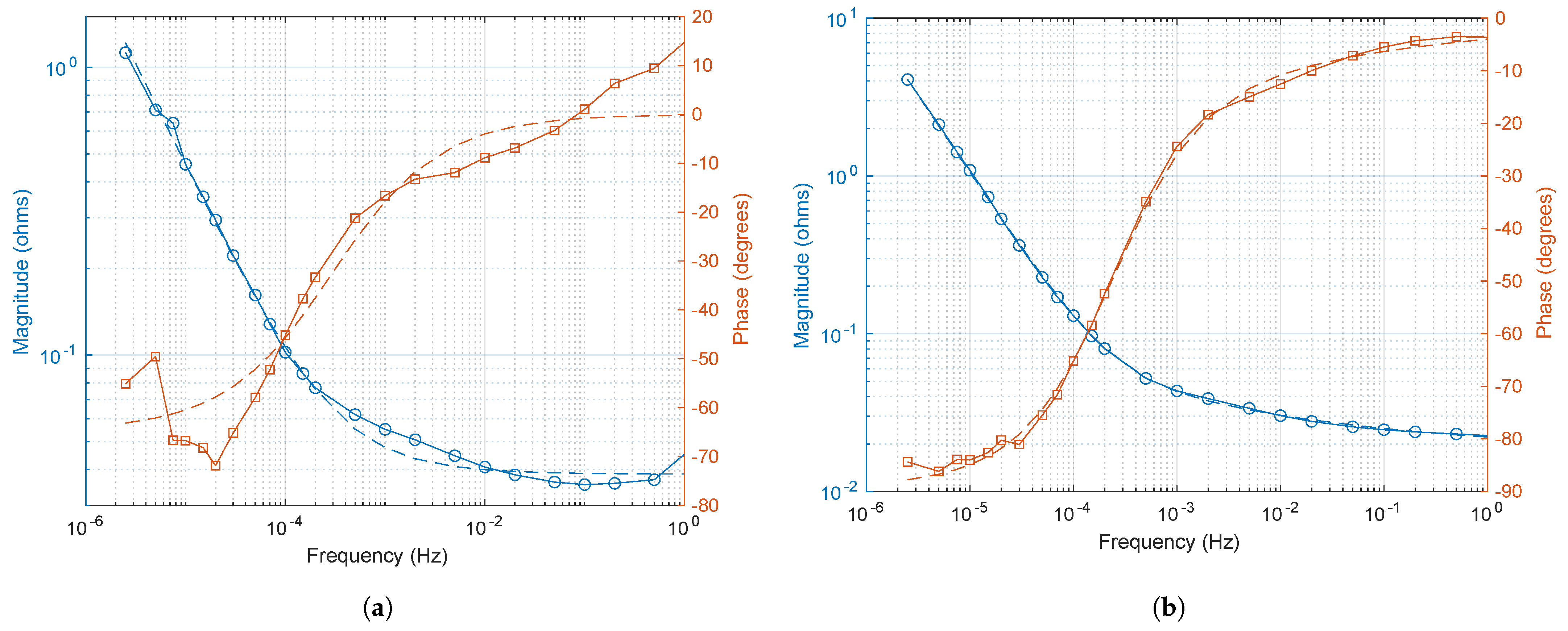
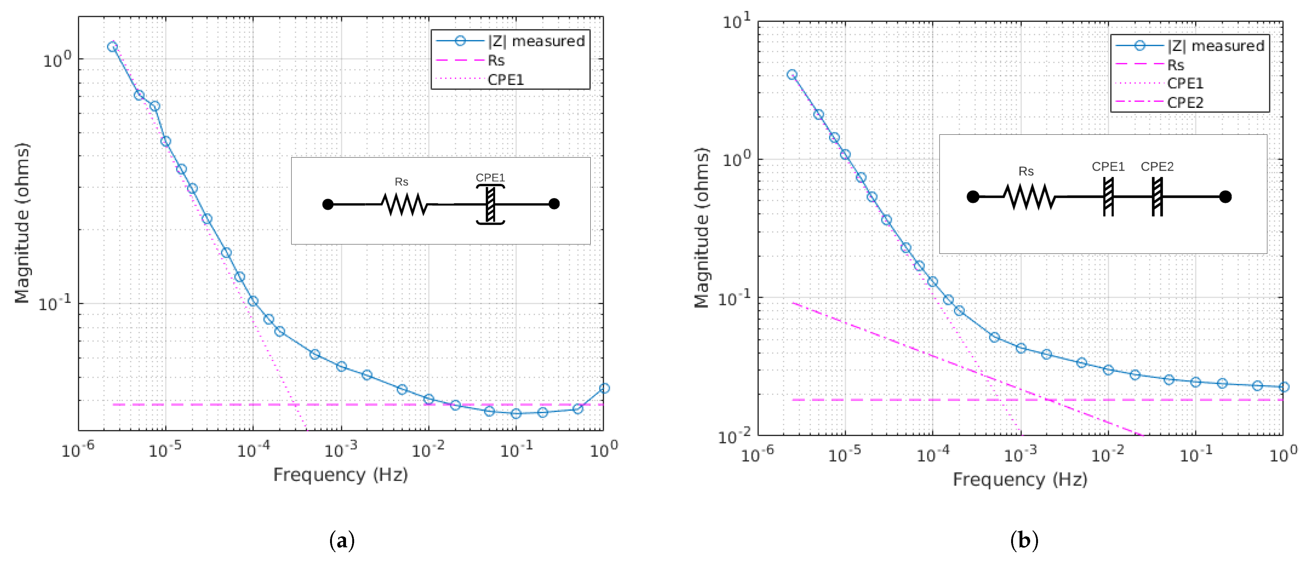
3.2. Conditions for Reliable EIS and ECM Fitting

Rate of charge movement is also crucial in EIS, particularly when carried out at the lowest frequencies. EIS is performed using sinusoidal tones (perturbations) which effectively correspond to the derivative $dV/dI$ of the battery characteristic at various frequencies (rates). This corresponds to the slope of the trace in a voltammogram. Traditional small-signal EIS measurement yields unreliable results, especially below 100 μHz, as described previously [16] and demonstrated by the example in Figure 3.

We suggest that this is because the slope of the voltammogram can vary sharply at sufficiently low rates. Addition of a large “working” square wave current in EIS measurement might shift the current-voltage characteristic away from the quasi-static state described above in Section 3.1. As shown by earlier published work [16], this has the effect of stabilizing impedance values.

Figure 4c shows, for example, that the value of impedance when the battery is at 4.0 V will be very different from the value at 4.1 V, since for a given increment in voltage the increment in current will be very different. The working current pulls the battery away from the small-signal, quasi-static condition, thus smoothing out the effect of the local peaks. The current is no longer “small”, but although the working current is large it reverses often enough for the net charge displacement it produces to remain small. Hence, the battery does not discharge before the measurement is complete, nor do its characteristics become nonlinear.

The implications of charge movement rates for EIS at ELFs are apparent when EIS is performed with and without working currents as described in Section 2.2. As shown in Figure 6a, with no working current (small measurement tones only, with the battery consequently in the quasi-static state as shown in Figure 4), poor quality magnitude and phase impedance plots are obtained. In particular, measured and fitted data do not match well for phase below 20 μHz and impedance magnitude above 100 mHz. An ECM based on two elements (R-CPE) only can be generated (

Table 1. ECM parameter estimation.

ECM	${\mathit{R}}_{\mathit{s}}$	$\mathit{\alpha }$	${\mathit{C}}_{\mathit{F}}$	${\mathit{C}}_2$	${\mathit{\alpha }}_2$	RMSE
bzdcp66 with 10 mA square wave (negligible working current)
R-CPE	38.53	0.7200	2397			0.1456
R-CPE-CPE	36.64	0.7445	3141	747.1	0.2731	0.1439
bzdcp66 with 500 mA square wave (working current)
R-CPE	26.80	0.9053	6160			0.1479
R-CPE-CPE	18.25	0.9913	14,250	155.3	0.2402	0.0296

CPE, constant-phase element; ECM, equivalent-circuit model; RMSE, root mean square error. $R_s$, series resistance ($ohm\times {10}^{-3}$); $C_F$ and $C_2$, fractional capacitances ($F/s^{(1-\alpha )}$) of first (R-CPE model) and second (R-CPE-CPE model) CPEs, with respective slopes denoted by $\alpha$ and ${\alpha }_2$.

), with no improvement in RMSE when a second CPE is added to the model.

Conversely, when the same measurement is made in the presence of a 500 mA square wave (which moves charge at much higher rates as with fast cycling as shown in Figure 5), stable and unambiguous magnitude and phase impedance plots are obtained (Figure 6b). Using these data, a three-element ECM (R-CPE-CPE) with a good fit to the measured data and substantial improvement in RMSE after addition of a second CPE can be generated (Table 1). These results replicate previously reported findings in lithium titanate batteries [16], and demonstrate that EIS at ELFs in an intact battery must be carried out in the presence of currents that would be expected when the battery is in use.

Note the substantial difference in $\alpha$ values between the 10 mA and 500 mA scenarios for the first CPE. With the 10 mA (negligible) square wave, the second CPE cannot be discerned, and the entire region of the Bode plot showing fractional capacitance has to be described using a single CPE with a “compromise” best-fit value of $\alpha \approx 0.7$. In the presence of the 500 mA square wave, two CPEs with more finely tuned and accurate values of $\alpha =0.99$ and $\alpha =0.24$ may be fitted.

The effect of the larger square-wave current begs the question as to what state the cell is in (i.e., is it now in a non–quasi-static state?). On one hand, there are relatively large “working” currents flowing (i.e., in the presence of the 500 mA square wave); on the other, those large currents reverse frequently, so that net charge flow is small over a period of minutes. In answer to this question, we contend that the system should be considered to be in a “pseudo–quasi-static” state, as evidenced by the reversible but asymmetric traces in CV-type plots that continue to show peaks that might correspond to individual electrode processes but that are greatly attenuated when compared with those seen in the presence of very small cycling currents (Figure 5c).

Fitted lines corresponding to the circuit elements in each ECM are shown in Figure 7a,b. Note in particular the impedance for CPE2 in Figure 7b. This element is discernible only through ELF measurement [16] and confirmed here to be visible only when the cell is not fully quasi-static but also not in perfect equilibrium, i.e., in the pseudo–quasi-static state described above. Certainly the data are not obscured by diffusion, but neither are the instantaneous currents small. We are in the region between “small-signal” measurements that typically apply to EIS work (that assumes a linear device), and the “large-signal” regime where nonlinear effects dominate.

We note here that the CPEs in this ECM do not represent physical elements inside the battery. The procedure essentially sees the cell as a “black box”, and uses the measured data to construct an electronic model with fractional capacitance based on as few elements as possible that can reproduce those data. We have demonstrated that a three-element, five-parameter ECM of the type shown here typically models real, measured data with good precision [11]. In terms of how the model relates to the cell’s charging behavior, the resistive part of the ECM reveals itself in the size of the instantaneous vertical jump in voltage on reversal of the current in Figure 5a. The curve following this jump and the roughly constant gradient $dV/dt$ later in each charging period (Figure 5a) correspond to the fractional capacitance effect of the CPEs.

4. Conclusions

These findings support the concept of equivalence of CV and ICA in terms of the information they provide to the experimenter. Both methods have associated rates and, in both cases, rate of charge movement is the key variable that determines what the investigator sees. Low rates of charge movement (with the cell consequently in a quasi-static state) yield detailed peaks corresponding to individual reactions in incremental charge or current plots, while greater rates lead to loss of resolution (as the cell transitions into a pseudo–quasi-static state) and the generation of plots more closely resembling CV as commonly presented in the literature. The current-controlled method with calculation of cumulative charge movement while the cell is in the pseudo–quasi-static state described in this manuscript may offer a practical solution, using basic equipment, to the problem of performing an analysis that might give information analogous to CV on an intact battery without risking destruction of the device under test.

Notwithstanding the difficulties mentioned above of attempting CV on a whole battery, we note here the recent work of Kim et al. [36], who have published CV profiles for four different battery types (including NCA). These tests were carried out at a low scan rate (0.05 mV/s) using commercially available battery testing and environmental control equipment with suitable safety features. The published NCA CV plot shows a hysteresis with three redox peaks corresponding to oxidation at the positive electrode, with corresponding reduction peaks, comparable to the plots shown in Figure 5 of the present manuscript. This would seem to confirm the potential utility of our suggested constant-current method, which does not require specialized and expensive commercial battery testing equipment, and to underline the importance of rate of movement of charge in terms of what the investigator sees.

Near-equilibrium quasi-static conditions are required to reveal electrode activity at different terminal voltages when performing ICA. However, these conditions interfere with small signal impedance measurements, or at least make them susceptible to small changes in equilibrium point, when we attempt EIS at ELFs. Attempts to fit ECMs using EIS data obtained under quasi-static conditions are therefore likely to result in unreliable models. In constrast to previous authors, who have suggested that ECMs with numerous components to represent individual electrochemical processes may be needed to model fractional devices such as batteries [10,24,25], we have shown that a simple ECM consisting of three elements only (R-CPE-CPE) is needed [11,16]. This ECM is discernible only via EIS performed at ELFs, and only when the cell is in the pseudo–quasi-static state (i.e., the conditions required for a CV-type analysis as described in this paper). Under the near-equilibrium quasi-static conditions that are required for ICA, EIS at ELFs is only partially successful in that the second CPE cannot be “seen”, and an R-CPE model, which is not sufficient to fully characterize the cell, only can be generated.

References

1. Atkins, P.W.; De Paula, J. Atkins’ Physical Chemistry, 8th ed.; Oxford University Press: Oxford, UK; New York, NY, USA, 2006. [Google Scholar]
2. Anonymous. Linear Sweep and Cyclic Voltammetry: The Principles. 2013. Available online: https://www.ceb.cam.ac.uk/research/groups/rg-eme/Edu/linear-sweep-and-cyclic-voltametry-the-principles (accessed on 21 May 2025).
3. Marken, F.; Neudeck, A.; Bond, A.M. Cyclic voltammetry. In Electroanalytical Methods: Guide to Experiments and Applications; Scholtz, F., Ed.; Springer: Berlin, Germany; New York, NY, USA, 2002. [Google Scholar]
4. Yu, D.Y.W.; Fietzek, C.; Weydanz, W.; Donoue, K.; Inoue, T.; Kurokawa, H.; Fujitani, S. Study of LiFePO4 by Cyclic Voltammetry. J. Electrochem. Soc. 2007, 154, A253. [Google Scholar] [CrossRef]
5. Kurzweil, P.; Scheuerpflug, W.; Frenzel, B.; Schell, C.; Schottenbauer, J. Differential Capacity as a Tool for SOC and SOH Estimation of Lithium Ion Batteries Using Charge/Discharge Curves, Cyclic Voltammetry, Impedance Spectroscopy, and Heat Events: A Tutorial. Energies 2022, 15, 4520. [Google Scholar] [CrossRef]
6. Ovejas, V.; Cuadras, A. Battery Aging Impedance Spectroscopy and Incremental Capacity Analysis. In Proceedings of the 10th International Workshop on Impedance Spectroscopy (IWIS): Chair of Measurement and Sensor Technology, Chemnitz, Germany, 26–29 September 2017. [Google Scholar]
7. Anseán, D.; García, V.M.; González, M.; Blanco-Viejo, C.; Viera, J.C.; Pulido, Y.F.; Sánchez, L. Lithium-Ion Battery Degradation Indicators Via Incremental Capacity Analysis. IEEE Trans. Ind. Appl. 2019, 55, 2992–3002. [Google Scholar] [CrossRef]
8. Vennam, G.; Sahoo, A.; Ahmed, S. A survey on lithium-ion battery internal and external degradation modeling and state of health estimation. J. Energy Storage 2022, 52, 104720. [Google Scholar] [CrossRef]
9. Zheng, L.; Zhu, J.; Lu, D.D.C.; Wang, G.; He, T. Incremental capacity analysis and differential voltage analysis based state of charge and capacity estimation for lithium-ion batteries. Energy 2018, 150, 759–769. [Google Scholar] [CrossRef]
10. Westerhoff, U.; Kurbach, K.; Lienesch, F.; Kurrat, M. Analysis of Lithium-Ion Battery Models Based on Electrochemical Impedance Spectroscopy. Energy Technol. 2016, 4, 1620–1630. [Google Scholar] [CrossRef]
11. Poihipi, E.; Scott, J.; Dunn, C. Distinguishability of Battery Equivalent-Circuit Models Containing CPEs: Updating the Work of Berthier, Diard, & Michel. J. Electroanal. Chem. 2022, 911, 116201. [Google Scholar] [CrossRef]
12. Talaie, E.; Bonnick, P.; Sun, X.; Pang, Q.; Liang, X.; Nazar, L.F. Methods and Protocols for Electrochemical Energy Storage Materials Research. Chem. Mater. 2017, 29, 90–105. [Google Scholar] [CrossRef]
13. Mauracher, P.; Karden, E. Dynamic modelling of lead/acid batteries using impedance spectroscopy for parameter identification. J. Power Sources 1997, 67, 69–84. [Google Scholar] [CrossRef]
14. Scott, J.; Hasan, R. New Results for Battery Impedance at Very Low Frequencies. IEEE Access 2019, 7, 106925–106930. [Google Scholar] [CrossRef]
15. Hasan, R.; Scott, J. Extending Randles’s Battery Model to Predict Impedance, Charge–Voltage, and Runtime Characteristics. IEEE Access 2020, 8, 85321–85328. [Google Scholar] [CrossRef]
16. Dunn, C.; Scott, J. Achieving Reliable and Repeatable Electrochemical Impedance Spectroscopy of Rechargeable Batteries at Extra-Low Frequencies. IEEE Trans. Instrum. Meas. 2022, 71, 1–8. [Google Scholar] [CrossRef]
17. Kim, T.; Choi, W.; Shin, H.C.; Choi, J.Y.; Kim, J.M.; Park, M.S.; Yoon, W.S. Applications of Voltammetry in Lithium Ion Battery Research. J. Electrochem. Sci. Technol 2020, 11, 14–25. [Google Scholar] [CrossRef]
18. Farrow, V. Characterisation of Rechargeable Batteries: Addressing Fractional Ultralow-Frequency Devices. Master’s Thesis, University of Waikato, Hamilton, New Zealand, 2020. [Google Scholar]
19. Scott, J.; Parker, A. Distortion analysis using SPICE. J. Audio Eng. Soc. 1995, 43, 1029–1040. [Google Scholar]
20. Randles, J.E.B. Kinetics of rapid electrode reactions. Discuss. Faraday Soc. 1947, 1, 11. [Google Scholar] [CrossRef]
21. Lasia, A. Dispersion of Impedances at Solid Electrodes. In Electrochemical Impedance Spectroscopy and Its Applications; Springer: New York, NY, USA, 2014; pp. 177–201. [Google Scholar] [CrossRef]
22. Westerlund, S.; Ekstam, L. Capacitor theory. IEEE Trans. Dielect. Electr. Insul. 1994, 1, 826–839. [Google Scholar] [CrossRef]
23. Jacquelin, J. The Phasance Concept. Curr. Top. Electrochem. 1997, 4, 127–136. [Google Scholar]
24. Choi, W.; Shin, H.C.; Kim, J.M.; Choi, J.Y.; Yoon, W.S. Modeling and Applications of Electrochemical Impedance Spectroscopy (EIS) for Lithium-ion Batteries. J. Electrochem. Sci. Technol. 2020, 11, 1–13. [Google Scholar] [CrossRef]
25. Gao, P.; Zhang, C.; Wen, G. Equivalent circuit model analysis on electrochemical impedance spectroscopy of lithium metal batteries. J. Power Sources 2015, 294, 67–74. [Google Scholar] [CrossRef]
26. Nelder, J.A.; Mead, R. A Simplex Method for Function Minimization. Comput. J. 1965, 7, 308–313. [Google Scholar] [CrossRef]
27. Press, W.H. Numerical Recipes in C: The Art of Scientific Computing, 2nd ed.; Cambridge University Press: Cambridge, UK, 1992. [Google Scholar]
28. Jiang, Y.; Jiang, J.; Zhang, C.; Zhang, W.; Gao, Y.; Guo, Q. Recognition of battery aging variations for LiFePO4 batteries in 2nd use applications combining incremental capacity analysis and statistical approaches. J. Power Sources 2017, 360, 180–188. [Google Scholar] [CrossRef]
29. Kalogiannis, T.; Stroe, D.I.; Nyborg, J.; Nørregaard, K.; Christensen, A.E.; Schaltz, E. Incremental Capacity Analysis of a Lithium-Ion Battery Pack for Different Charging Rates. ECS Trans. 2017, 77, 403–412. [Google Scholar] [CrossRef]
30. Krupp, A.; Ferg, E.; Schuldt, F.; Derendorf, K.; Agert, C. Incremental Capacity Analysis as a State of Health Estimation Method for Lithium-Ion Battery Modules with Series-Connected Cells. Batteries 2020, 7, 2. [Google Scholar] [CrossRef]
31. Maures, M.; Zhang, Y.; Martin, C.; Delétage, J.Y.; Vinassa, J.M.; Briat, O. Impact of temperature on calendar ageing of Lithium-ion battery using incremental capacity analysis. Microelectron. Reliab. 2019, 100–101, 113364. [Google Scholar] [CrossRef]
32. Zhang, Y.C.; Briat, O.; Delétage, J.Y.; Martin, C.; Chadourne, N.; Vinassa, J.M. Efficient state of health estimation of Li-ion battery under several ageing types for aeronautic applications. Microelectron. Reliab. 2018, 88–90, 1231–1235. [Google Scholar] [CrossRef]
33. Schaltz, E.; Stroe, D.I.; Norregaard, K.; Ingvardsen, L.S.; Christensen, A. Incremental Capacity Analysis Applied on Electric Vehicles for Battery State-of-Health Estimation. IEEE Trans. Ind. Appl. 2021, 57, 1810–1817. [Google Scholar] [CrossRef]
34. Plattard, T.; Barnel, N.; Assaud, L.; Franger, S.; Duffault, J.M. Combining a Fatigue Model and an Incremental Capacity Analysis on a Commercial NMC/Graphite Cell under Constant Current Cycling with and without Calendar Aging. Batteries 2019, 5, 36. [Google Scholar] [CrossRef]
35. Huang, M. Incremental Capacity Analysis-Based Impact Study of Diverse Usage Patterns on Lithium-Ion Battery Aging in Electrified Vehicles. Batteries 2019, 5, 59. [Google Scholar] [CrossRef]
36. Kim, N.; Shamim, N.; Crawford, A.; Viswanathan, V.V.; Sivakumar, B.M.; Huang, Q.; Reed, D.; Sprenkle, V.; Choi, D. Comparison of Li-ion battery chemistries under grid duty cycles. J. Power Sources 2022, 546, 231949. [Google Scholar] [CrossRef]
Figure 1. System architecture.
Metrology 05 00031 g001
Figure 2. 3000-s segment of a time domain plot to illustrate the use of a small-signal sinusoidal multitone superimposed on a 1.5 A 1720 μHz square wave “working” current.
Metrology 05 00031 g002
Figure 3. Magnitude and phase impedance curves from extra-low frequency (down to 20 μHz) electrochemical impedance spectroscopy on a 4.0 Ah lithium iron phosphate (LiFePO4) 26700 battery. This example shows results from consecutive measurements on the same cell with (a) a small-signal measurement multitone stimulus only, and (b) the same small signal multitone superimposed on a 1320 μHz 3.0 A square wave. Note the variability between measurements in (a), particularly in phase results and especially at the lowest frequencies. In (b), increasing impedance magnitude and phase changes at very low frequencies with each successive measurement reflect changing impedance characteristics of the battery with ongoing use.
Metrology 05 00031 g003aMetrology 05 00031 g003b
Figure 4. 4.8 Ah lithium NCA cell cycled with a charge/discharge current of 100 mA (C/48). (a) Cycling plot: cell current and voltage versus time. (b) Incremental capacity versus cell voltage (ICA plot). (c) Current versus cell voltage (CV-type plot).
Metrology 05 00031 g004
Figure 5. 4.8 Ah lithium NCA cell cycled with a charge/discharge current of 5 A (approximately 1C): three complete cycles. (a) Cycling plot: cell current and voltage versus time (one of three complete cycles). (b) Incremental capacity versus cell voltage (ICA plot). (c) Current versus cell voltage (CV-type plot).
Metrology 05 00031 g005
Figure 6. Measured (solid lines) and fitted (dashed lines) magnitude (open circles) and phase (open squares) impedance curves: extra-low frequency (down to 2.5 μHz) electrochemical impedance spectroscopy on a 4.8 Ah lithium NCA cell. (a) Measurement multitone superimposed on a negligible (10 mA) square wave current. (b) Measurement multitone superimposed on a 500 mA square wave “working” current.
Metrology 05 00031 g006
Figure 7. Measured impedance magnitude with fitted lines showing discernible equivalent circuit elements: 4.8 Ah lithium NCA cell. (a) Measurement multitone superimposed on a negligible (10 mA) square wave. (b) Measurement multitone superimposed on a 500 mA square wave “working” current.
Metrology 05 00031 g007