
Learning-Based 3D Reconstruction Methods for Non-Collaborative Surfaces—A Metrological Evaluation
 , ,
, ,  and
and 
Abstract
1. Introduction
- (i)
- to report the available learning-based methods for the 3D reconstruction of industrial objects and, in general, non-collaborative surfaces.
- (ii)
- to objectively evaluate the quality of 3D reconstructions generated by NeRF, MVS, MDE, GS, and generative AI methods.
- (iii)
- to provide a clear summary of the advantages and limitations of such methods for 3D metrology tasks.
2. State of the Art
2.1. NeRF
2.1.1. Multi-View Dependent NeRF
2.1.2. Few/Single Shot NeRF
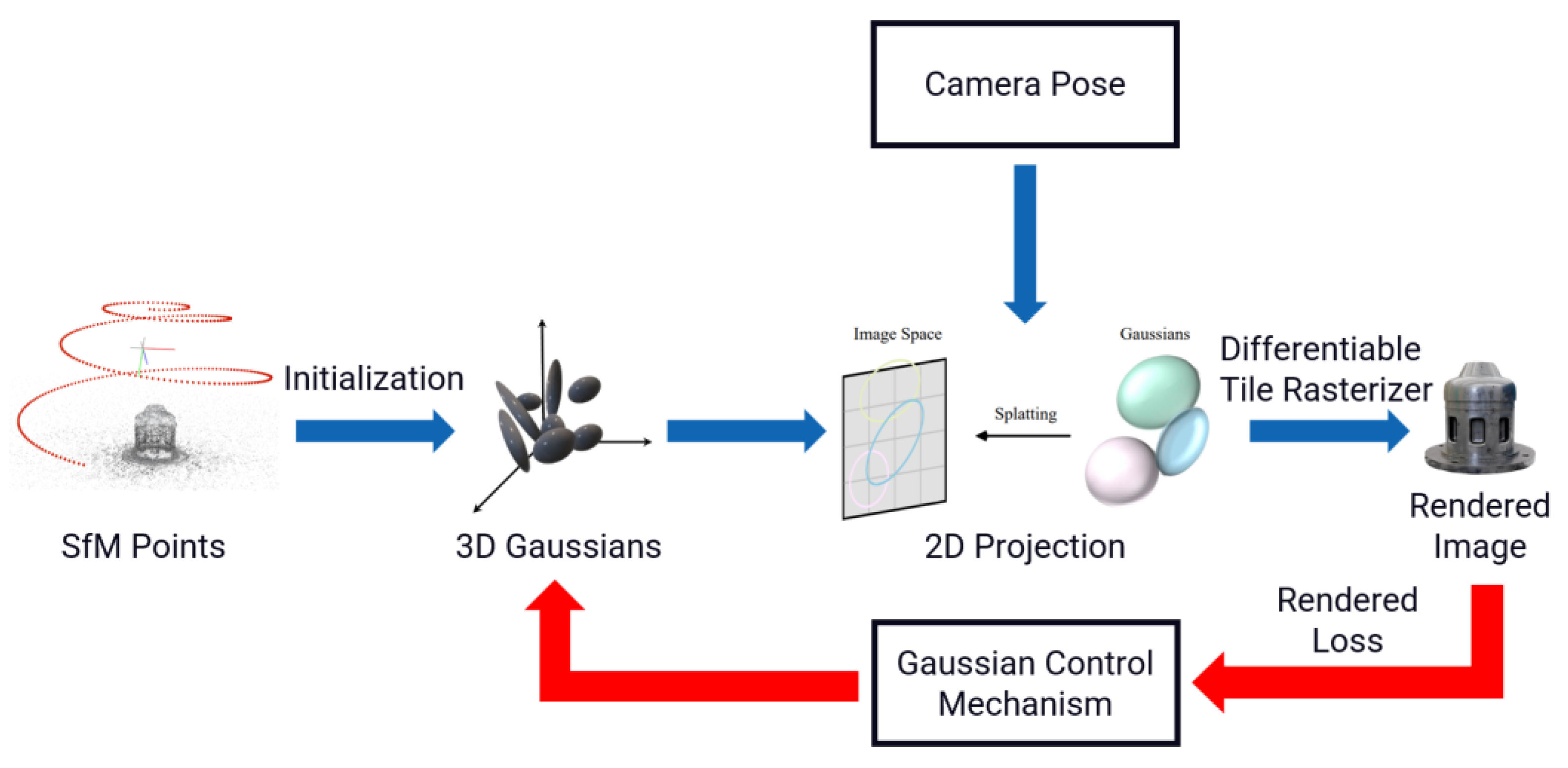
2.2. Gaussian Splatting (GS)
2.3. Learning-Based MVS
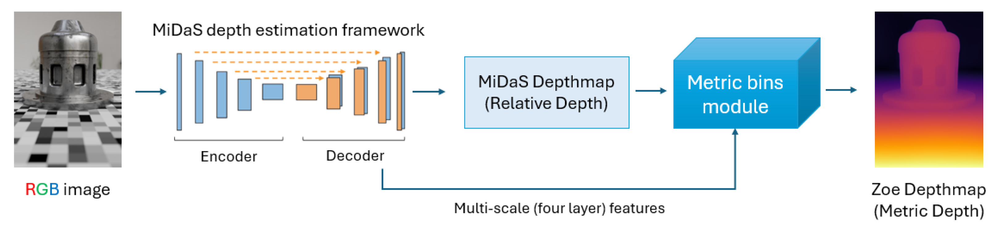
2.4. Monocular Depth Estimation (MDE)
2.5. Generative AI
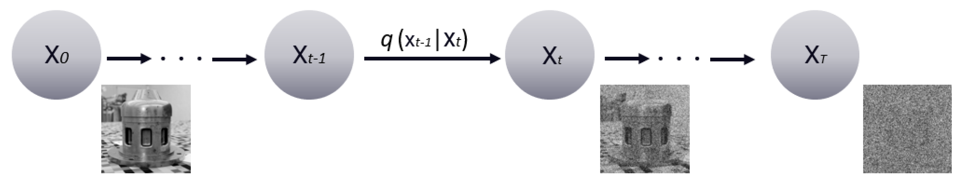
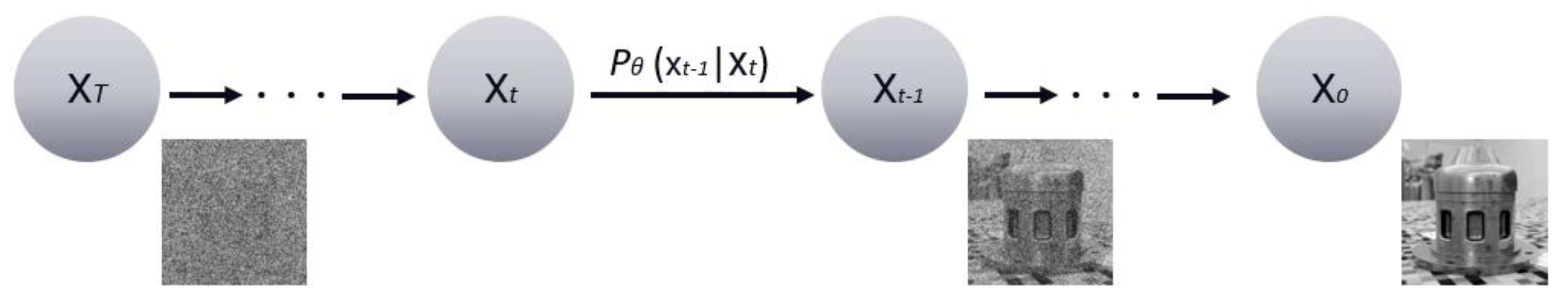
2.5.1. Diffusion Model
2.5.2. Image-to-3D by Diffusion Prior
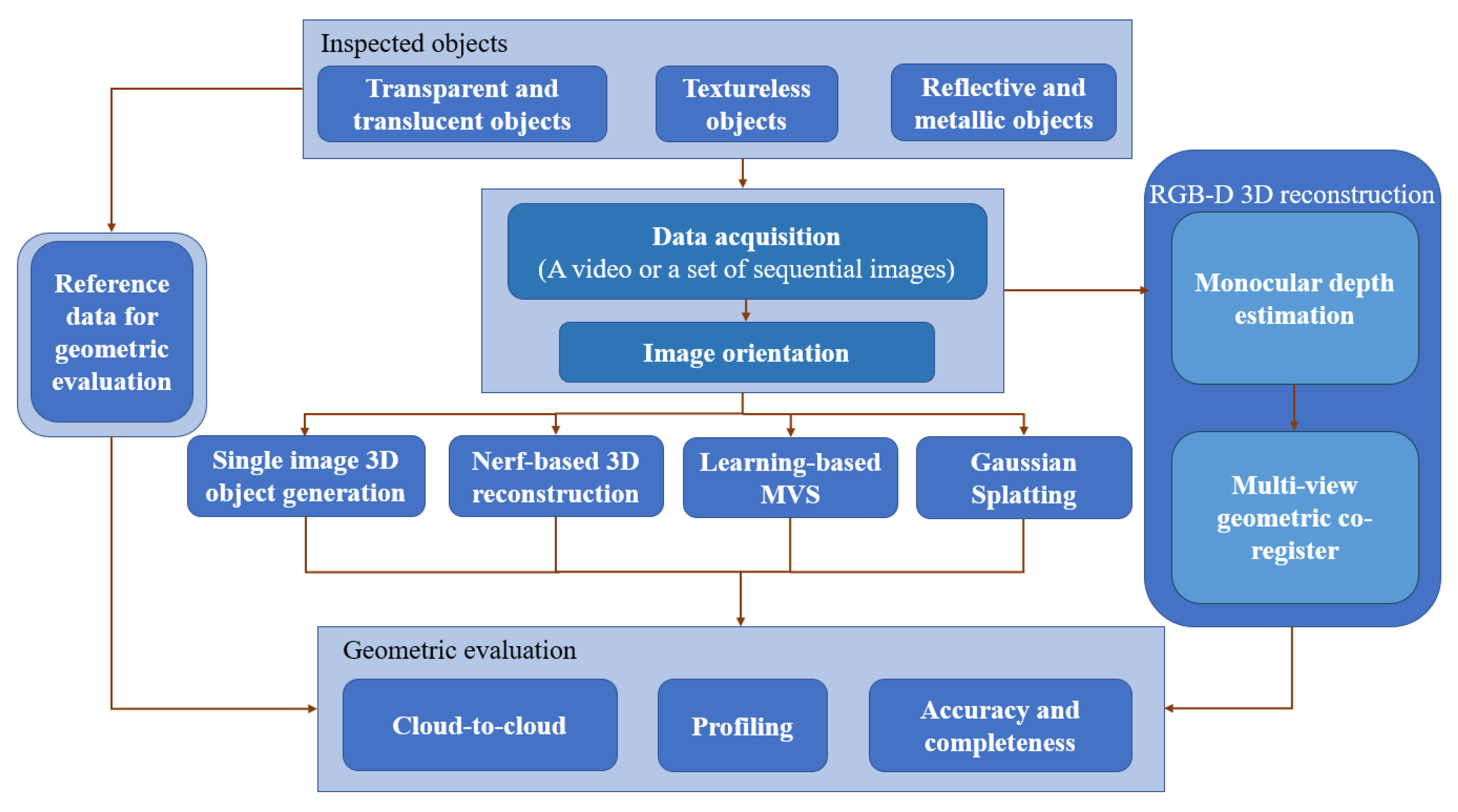
3. Analysis and Evaluation Methodology
3.1. Proposed Assessment Methodology
3.2. Metrics
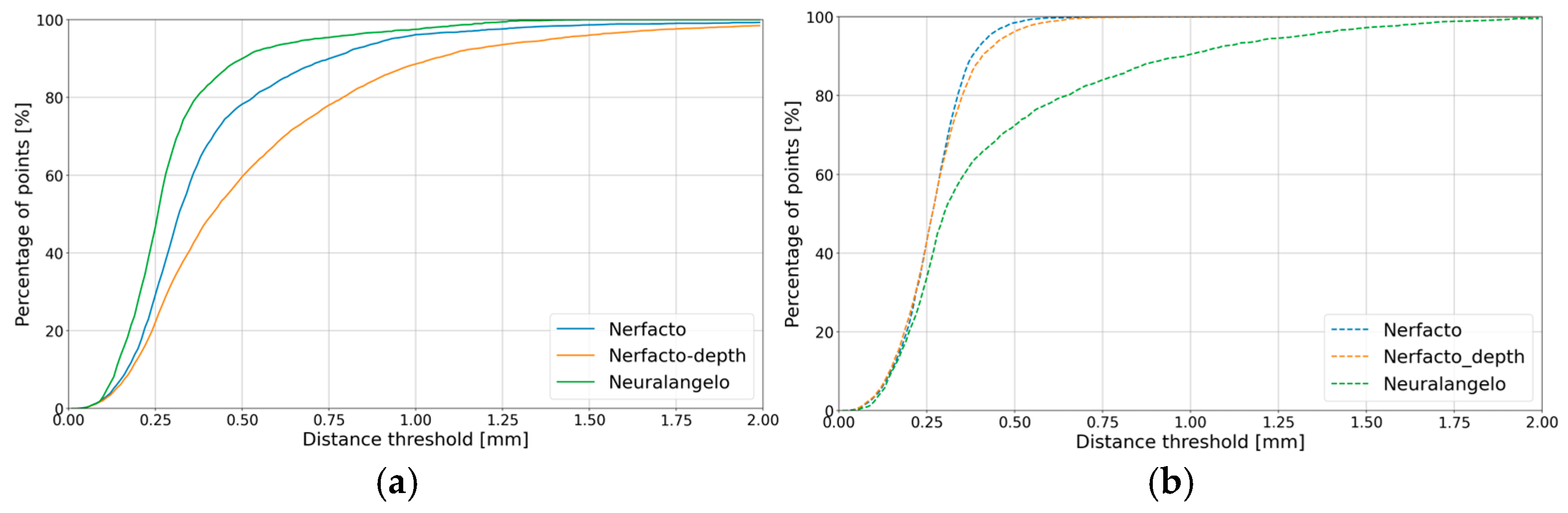
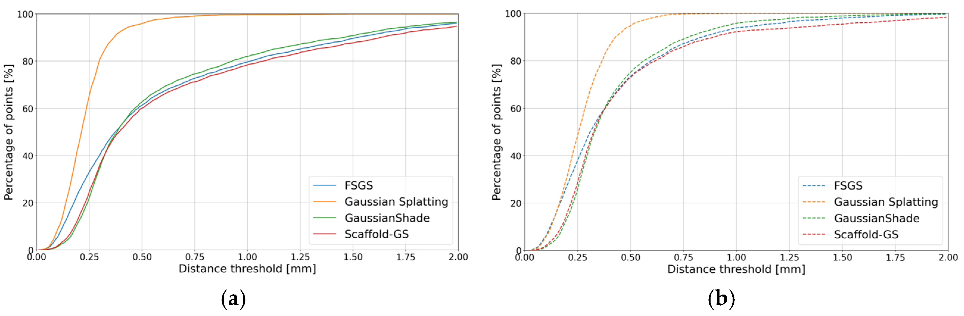
4. Comparison and Analysis
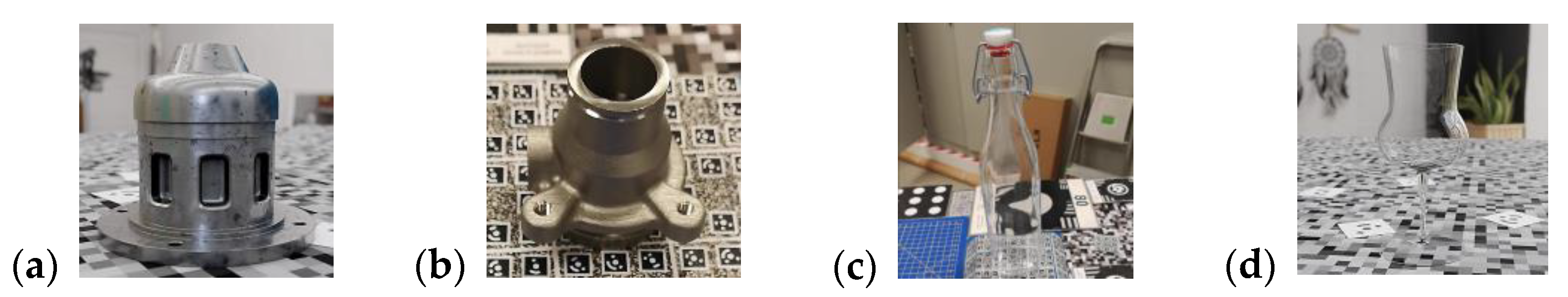
4.1. Testing Objects and Methods
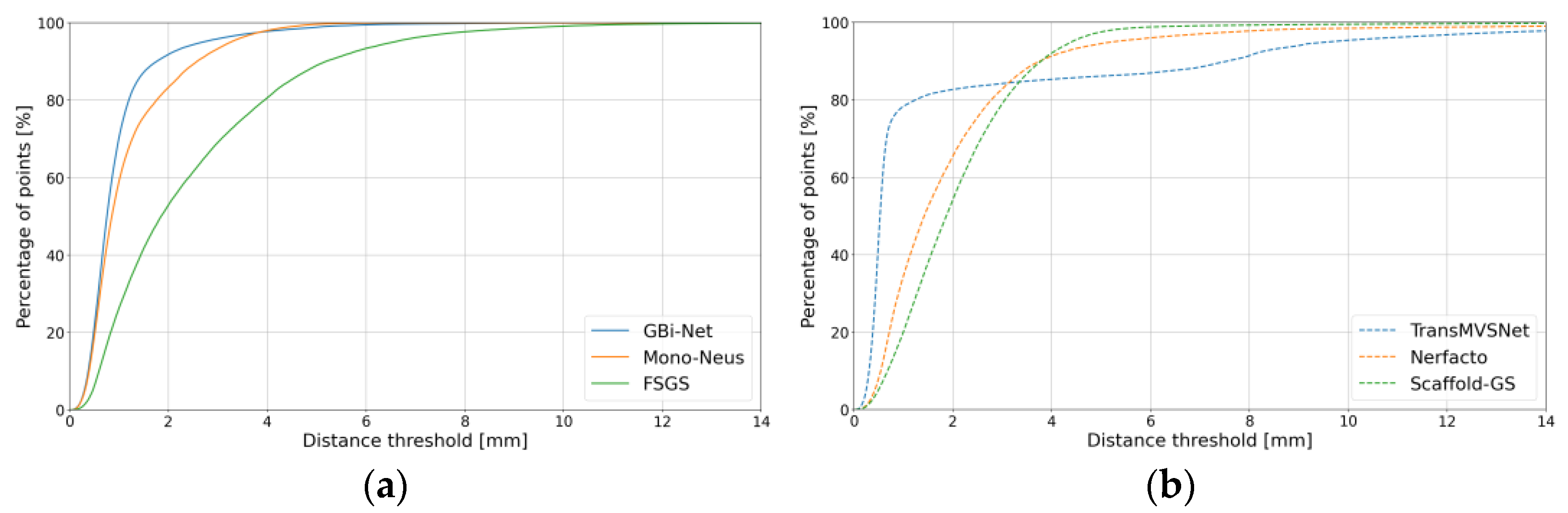
4.2. The 3D Results from Multi-View Image Sequences (NeRF, GS, Learning-Based MVS)
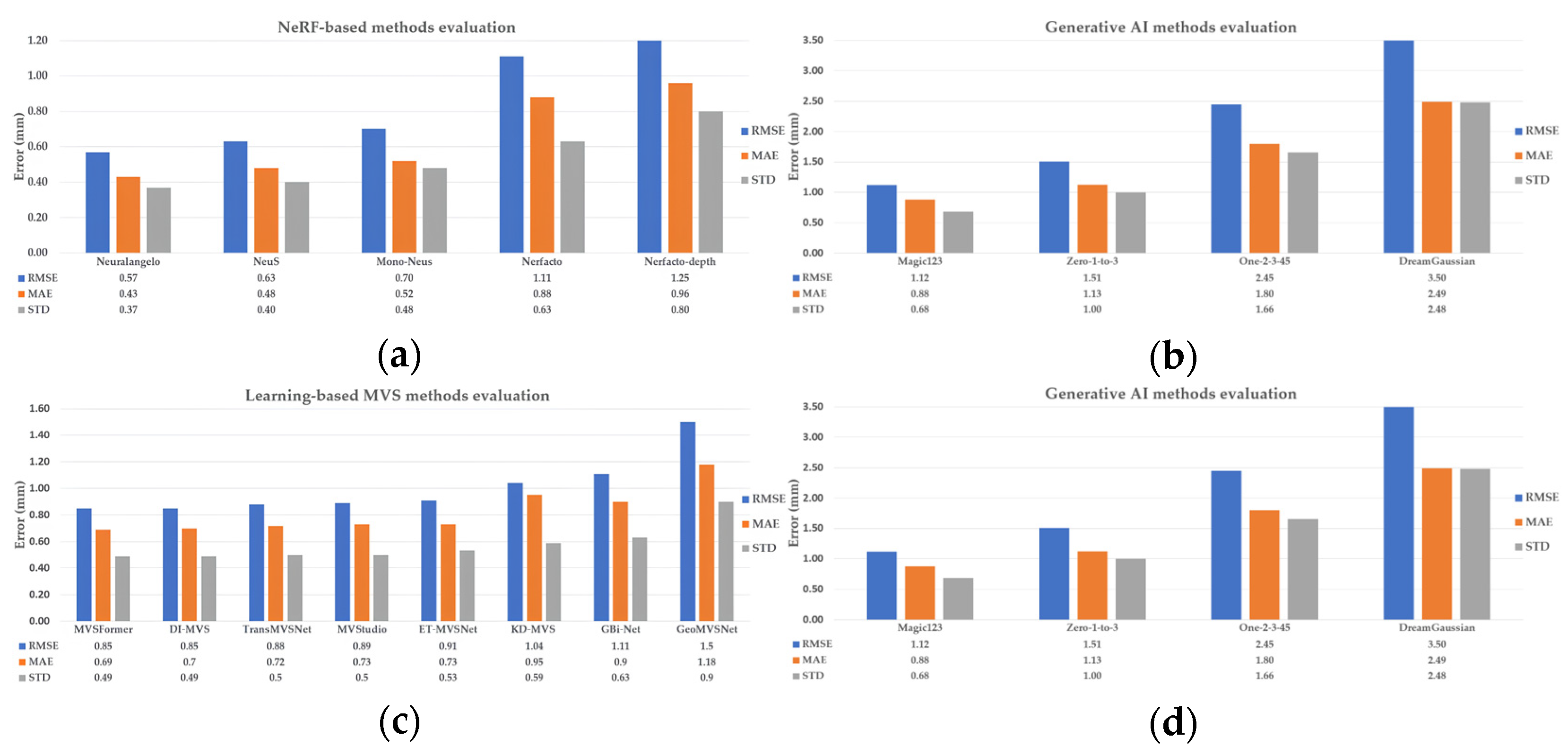
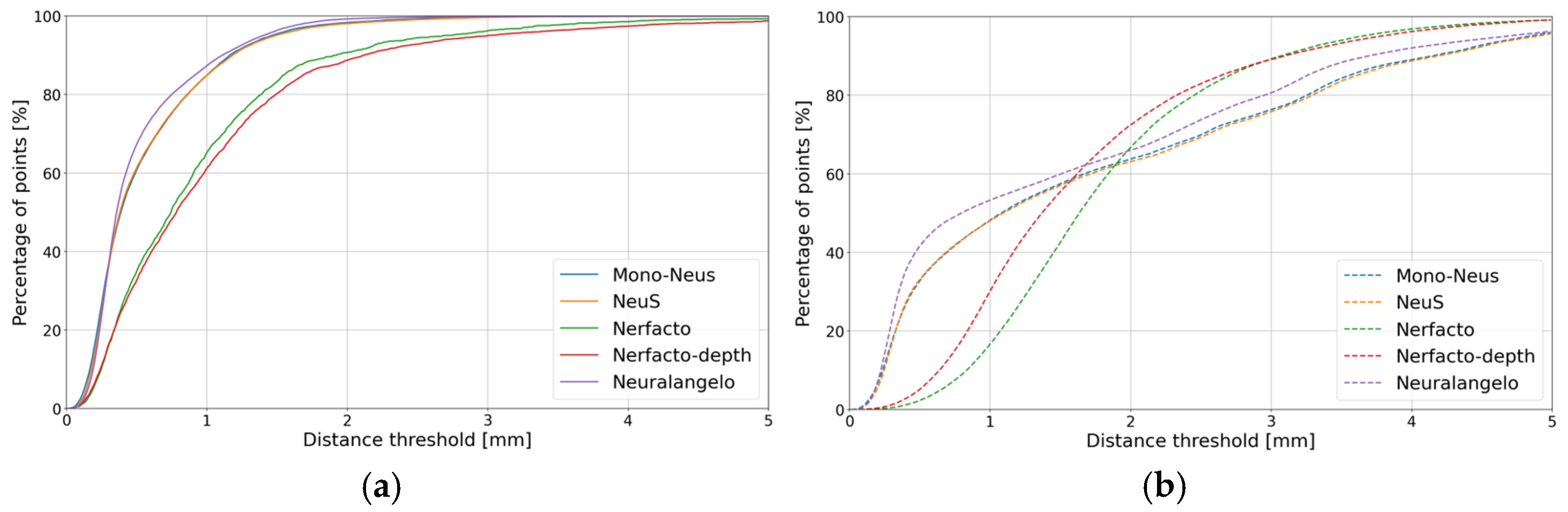
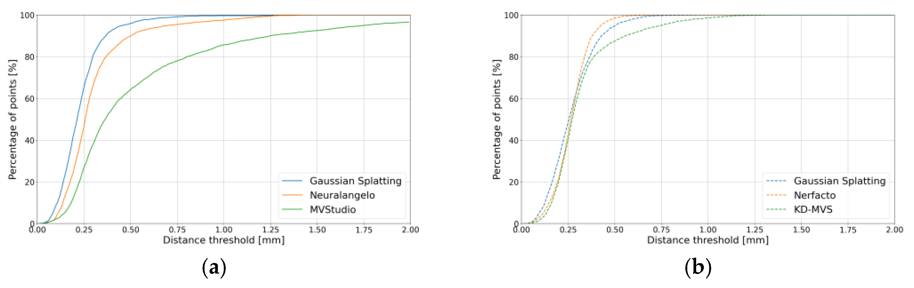
4.2.1. Industrial_A Object
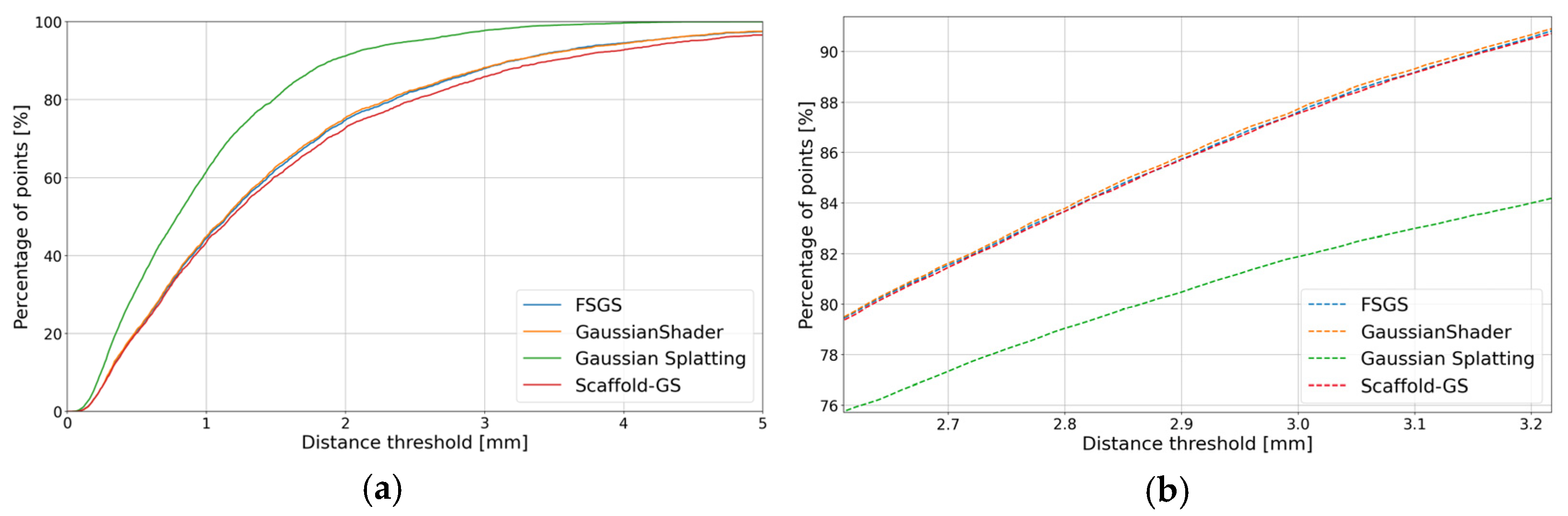
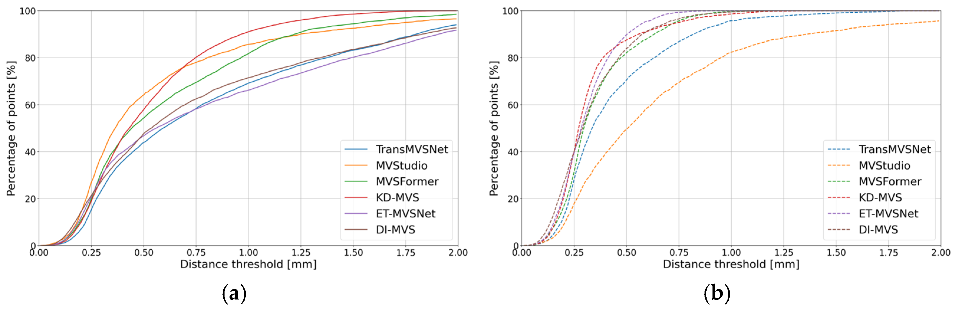
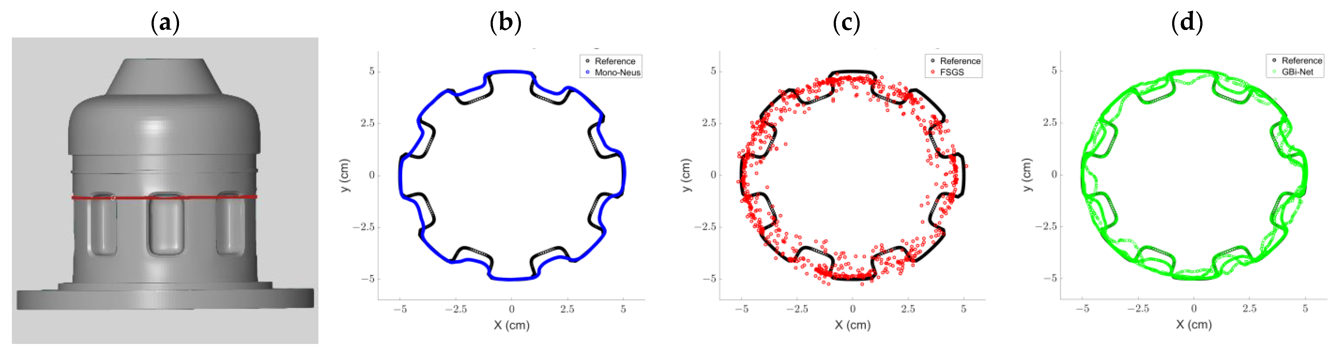
4.2.2. Metallic Object
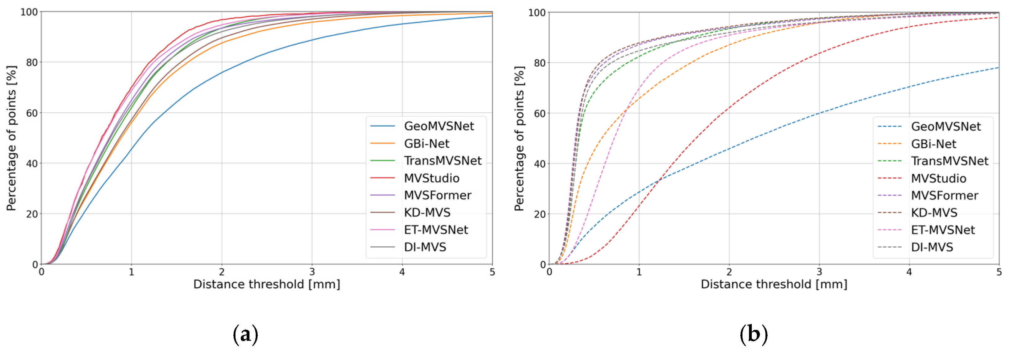
4.2.3. Transparent Object
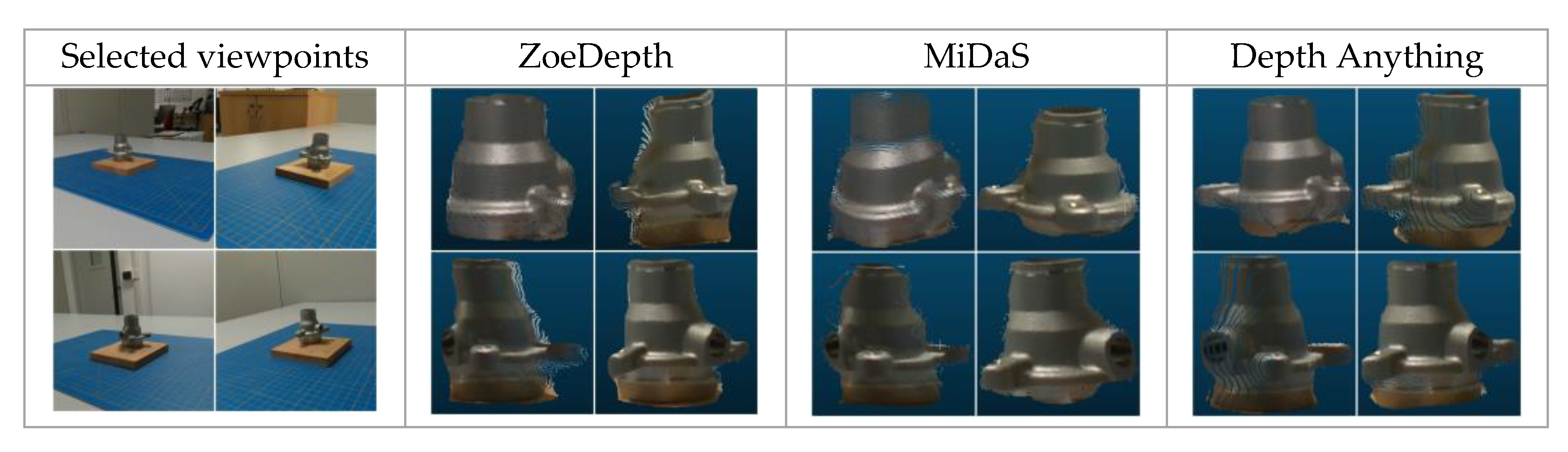
4.3. The 3D Results from Monocular Depth Estimation (MDE)
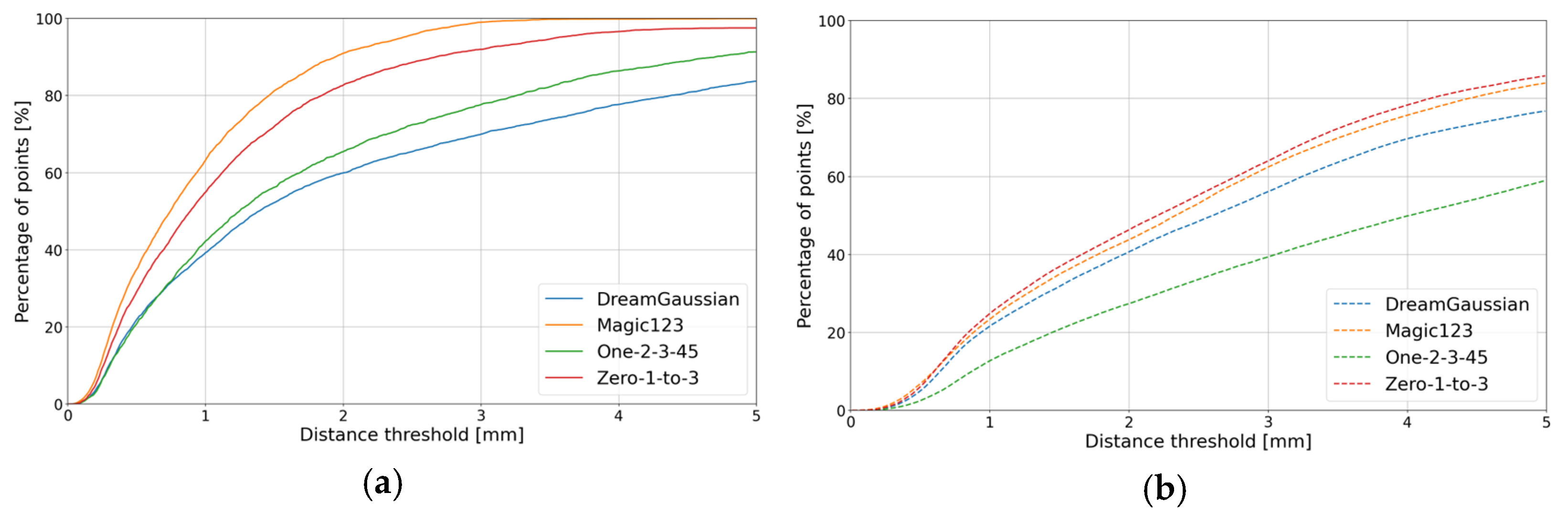
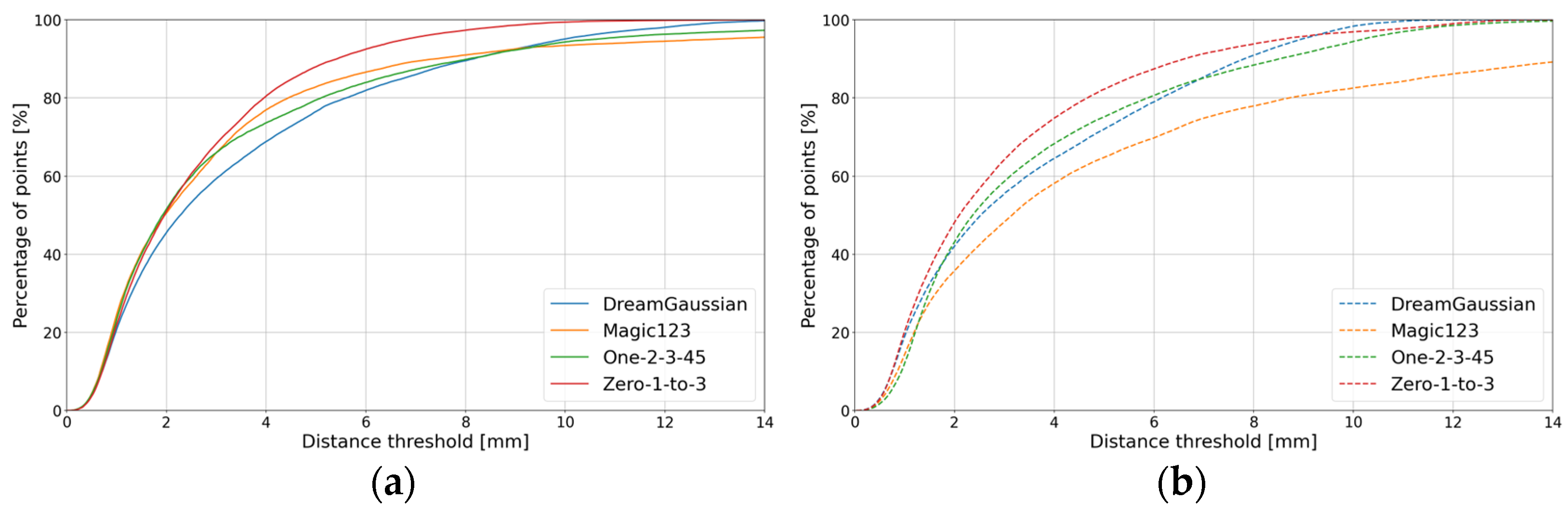
4.4. The 3D Results from Novel View Synthesis (Generative AI)
5. Discussion
6. Conclusions and Future Research Lines
Author Contributions
Funding
Data Availability Statement
Conflicts of Interest
Appendix A
Appendix A.1. Industrial_A Object
Appendix A.2. Synthetic_Metallic Objects


Appendix A.3. Synthetic_Glass Objects

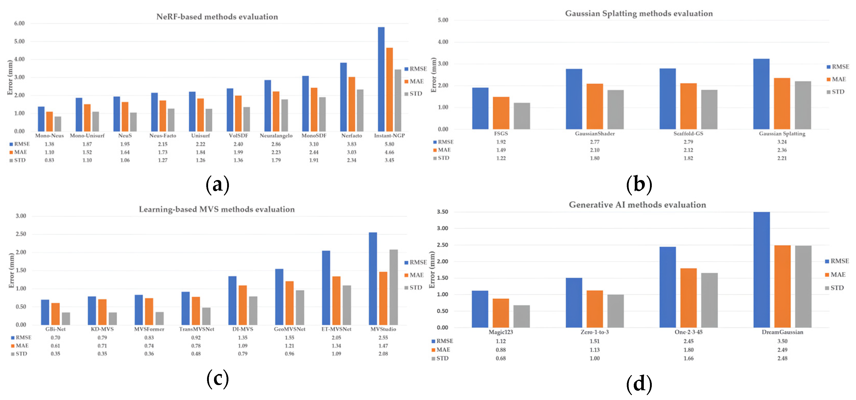
| Method | 3D Geometry | Comparison Result [mm] | Metric [mm] | |||
|---|---|---|---|---|---|---|
| RMSD | MAE | STD | Mean_E | |||
| Nerfacto | 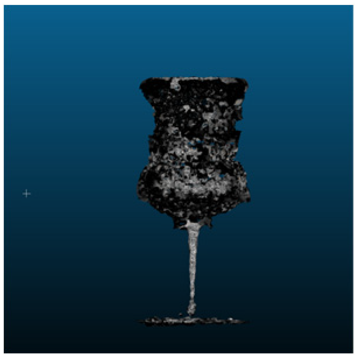 | 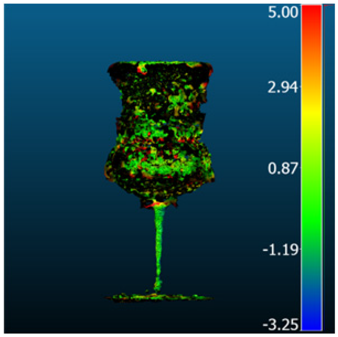 | 3.2 | 2.43 | 2.08 | 1.98 |
| Nerfacto-depth | 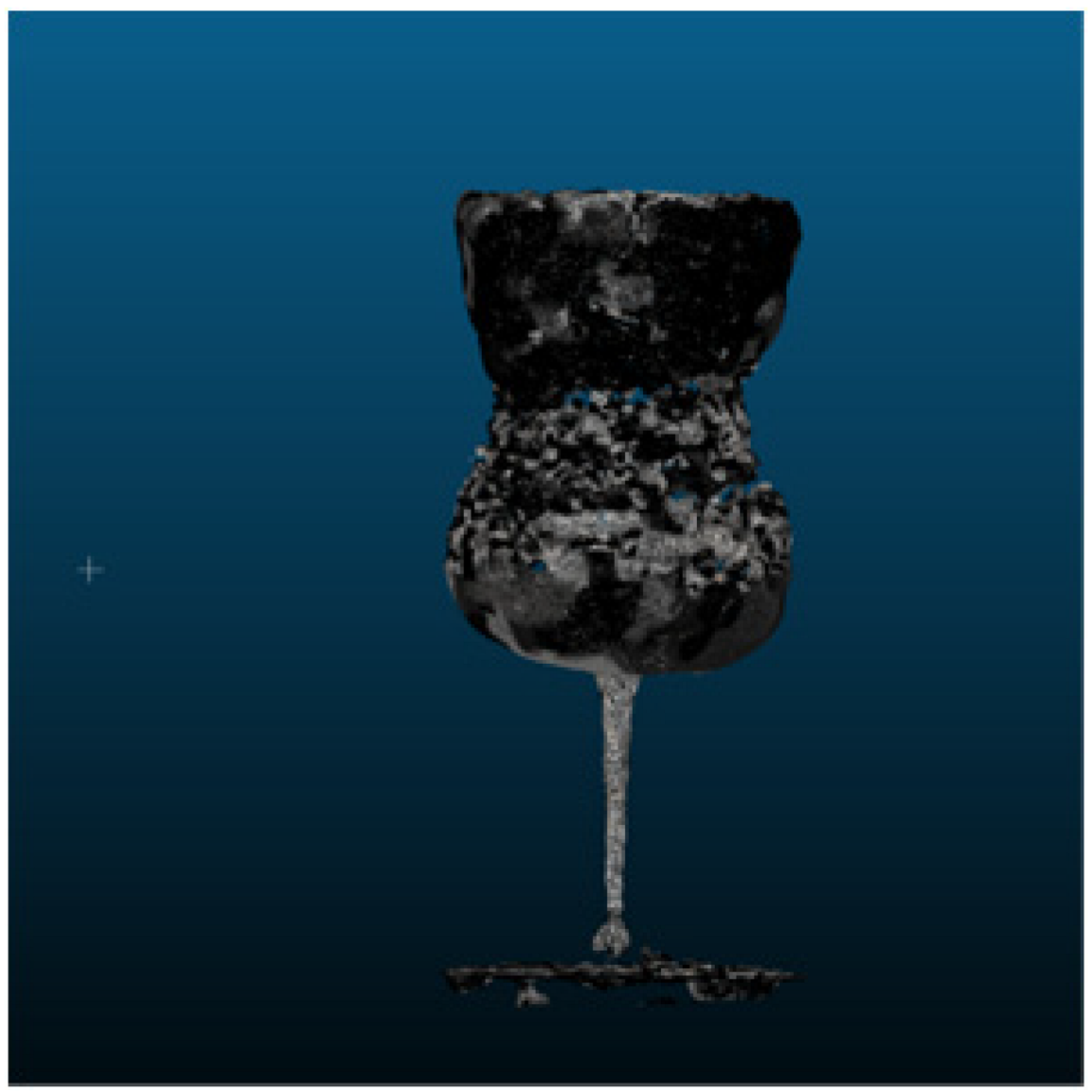 | 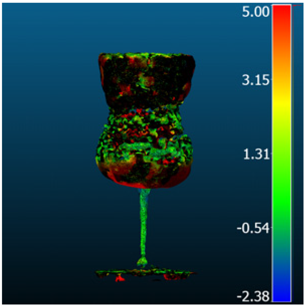 | 5.03 | 3.76 | 3.33 | 3.40 |
| Neuralangelo | 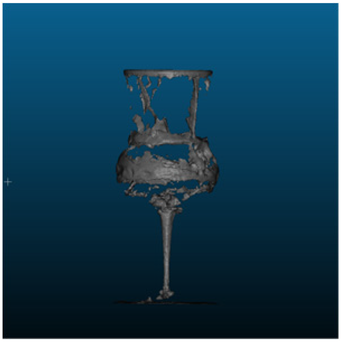 | 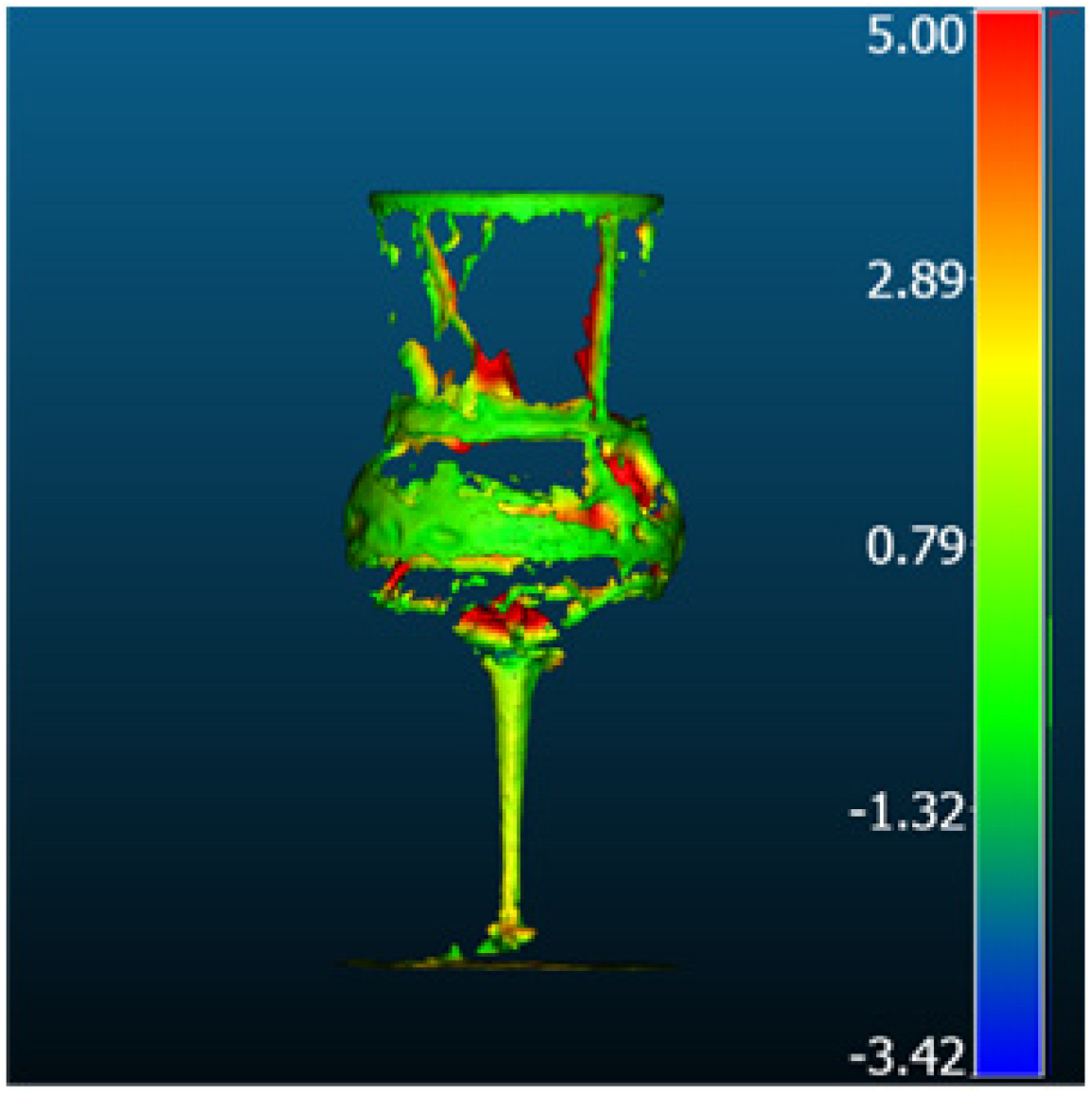 | 2.29 | 1.72 | 1.51 | 1.19 |
| Method | 3D Geometry | Comparison Result [mm] | Metric [mm] | |||
|---|---|---|---|---|---|---|
| RMSD | MAE | STD | Mean_E | |||
| FSGS | 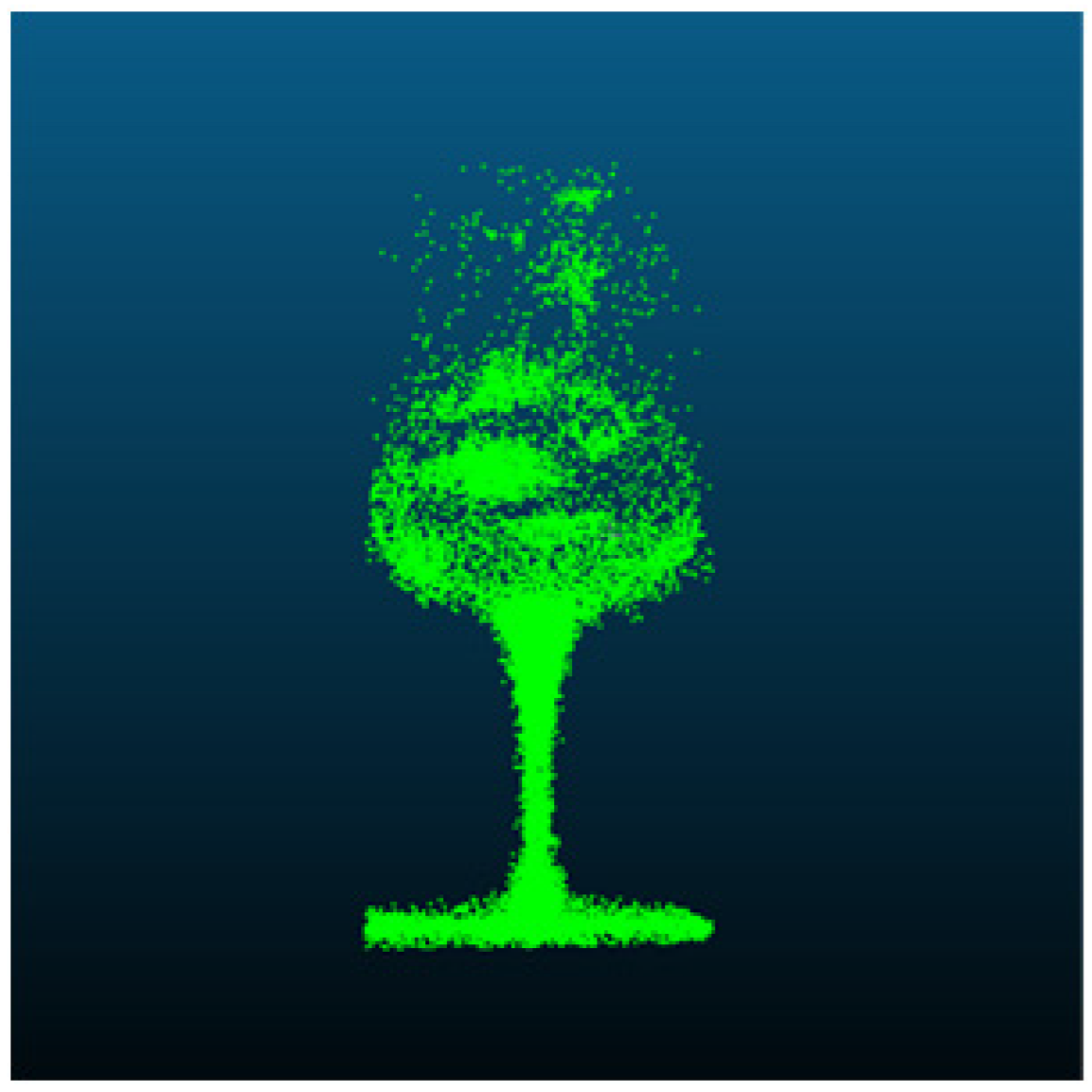 | 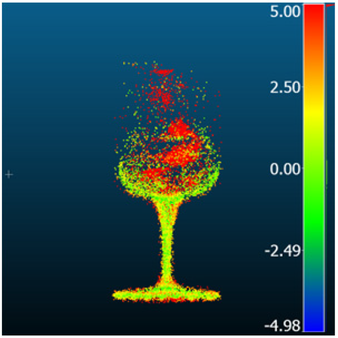 | 5.78 | 3.63 | 4.5 | 2.9 |
| GaussianShader | 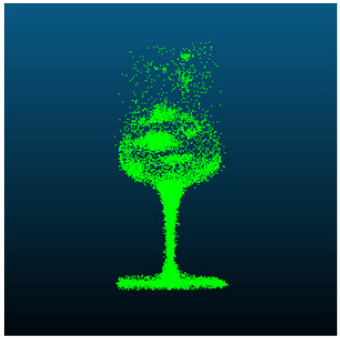 | 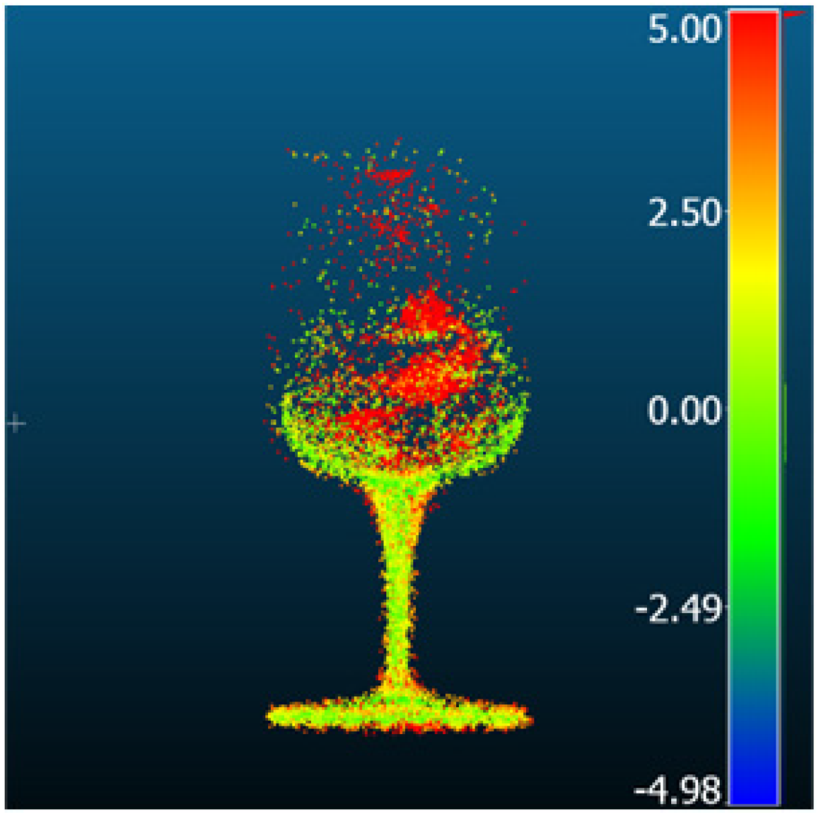 | 5.39 | 3.4 | 4.18 | 2.63 |
| Gaussian Splatting | 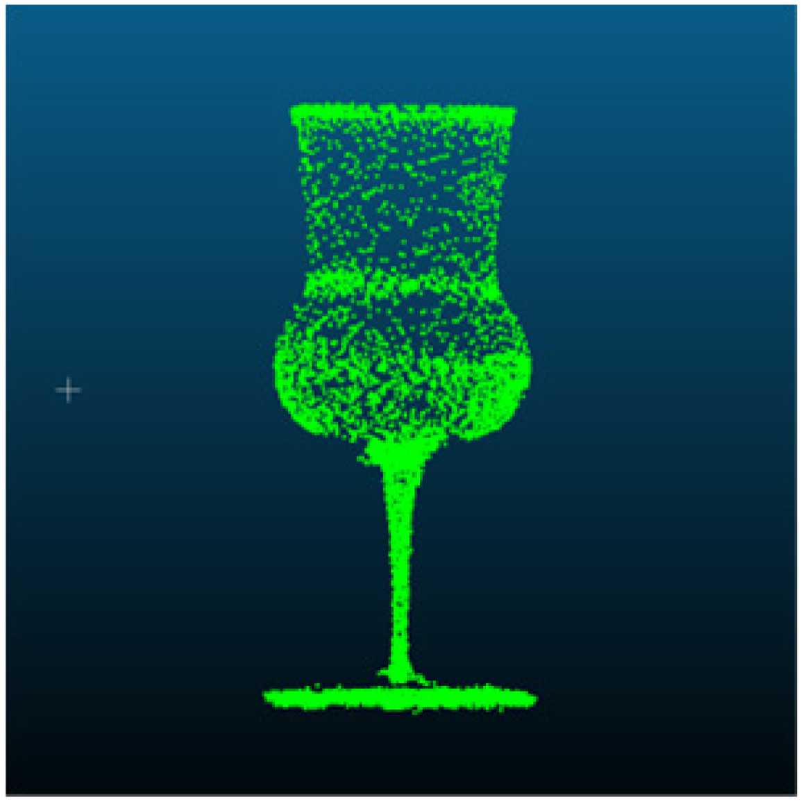 | 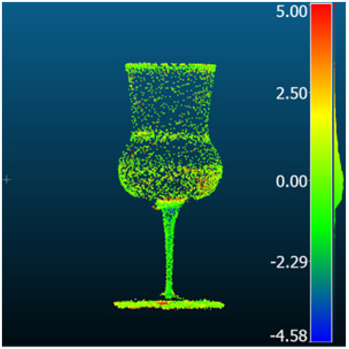 | 1.54 | 1.22 | 0.93 | 0.44 |
| Scaffold-GS | 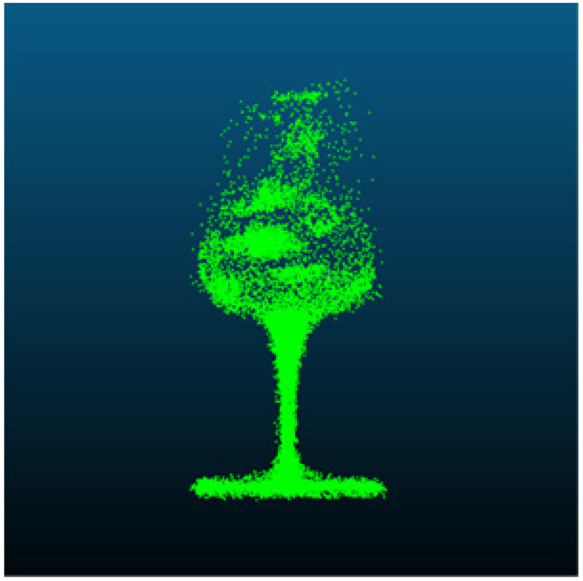 |  | 6.16 | 3.84 | 4.81 | 3.13 |
| Method | 3D Geometry | Comparison Result [mm] | Metric [mm] | |||
|---|---|---|---|---|---|---|
| RMSD | MAE | STD | Mean_E | |||
| ET-MVSNet | 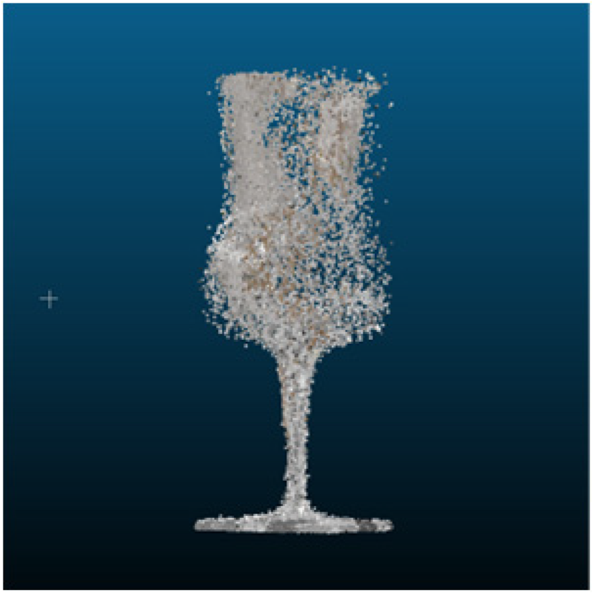 | 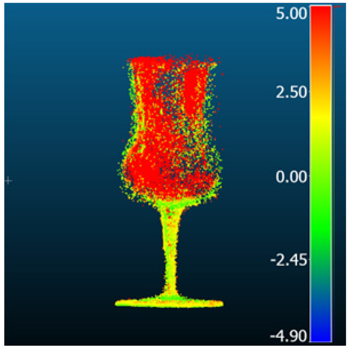 | 9.49 | 6.31 | 7.08 | 5.82 |
| MVStudio |  | 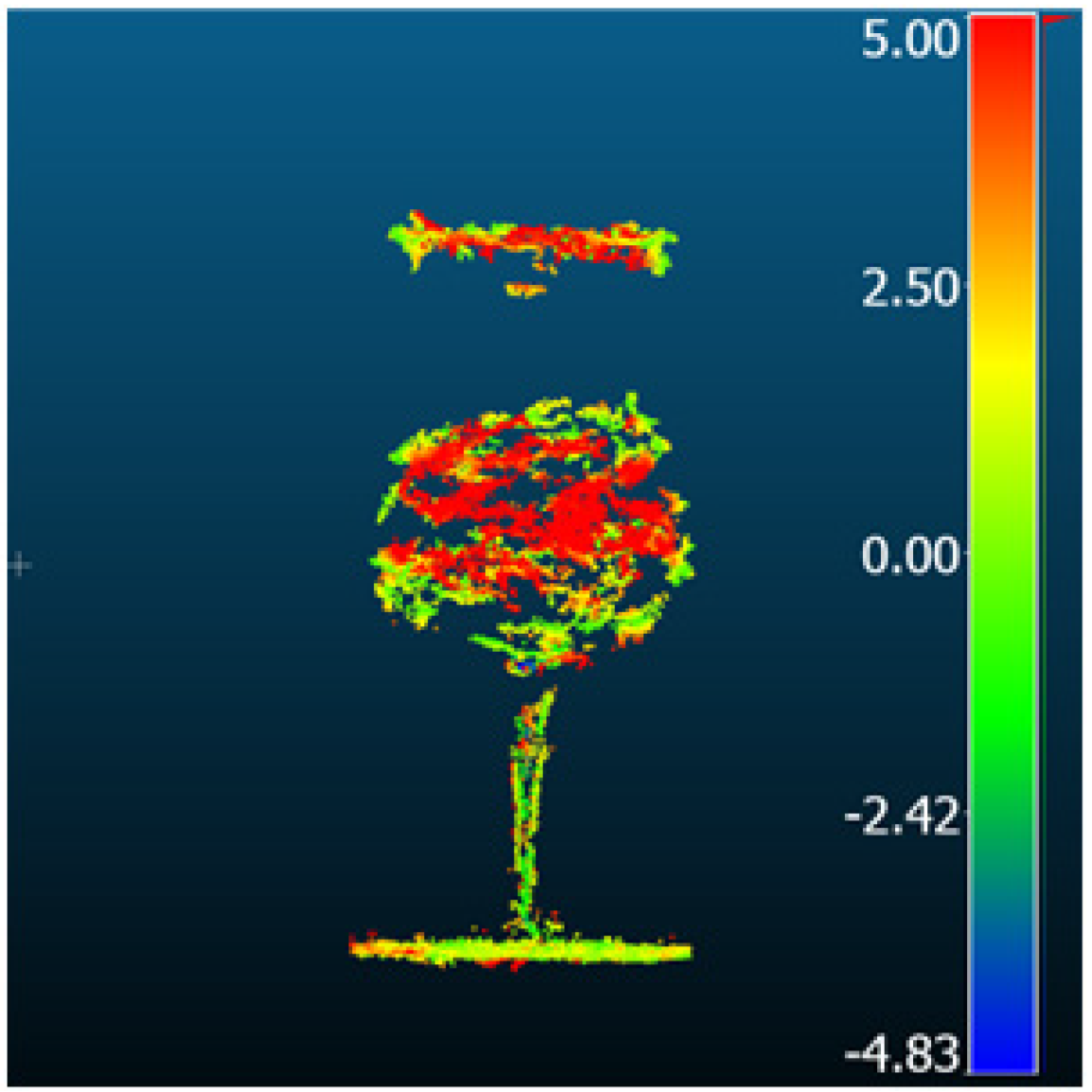 | 3.14 | 1.69 | 1.43 | 0.93 |
| TransMVSNet | 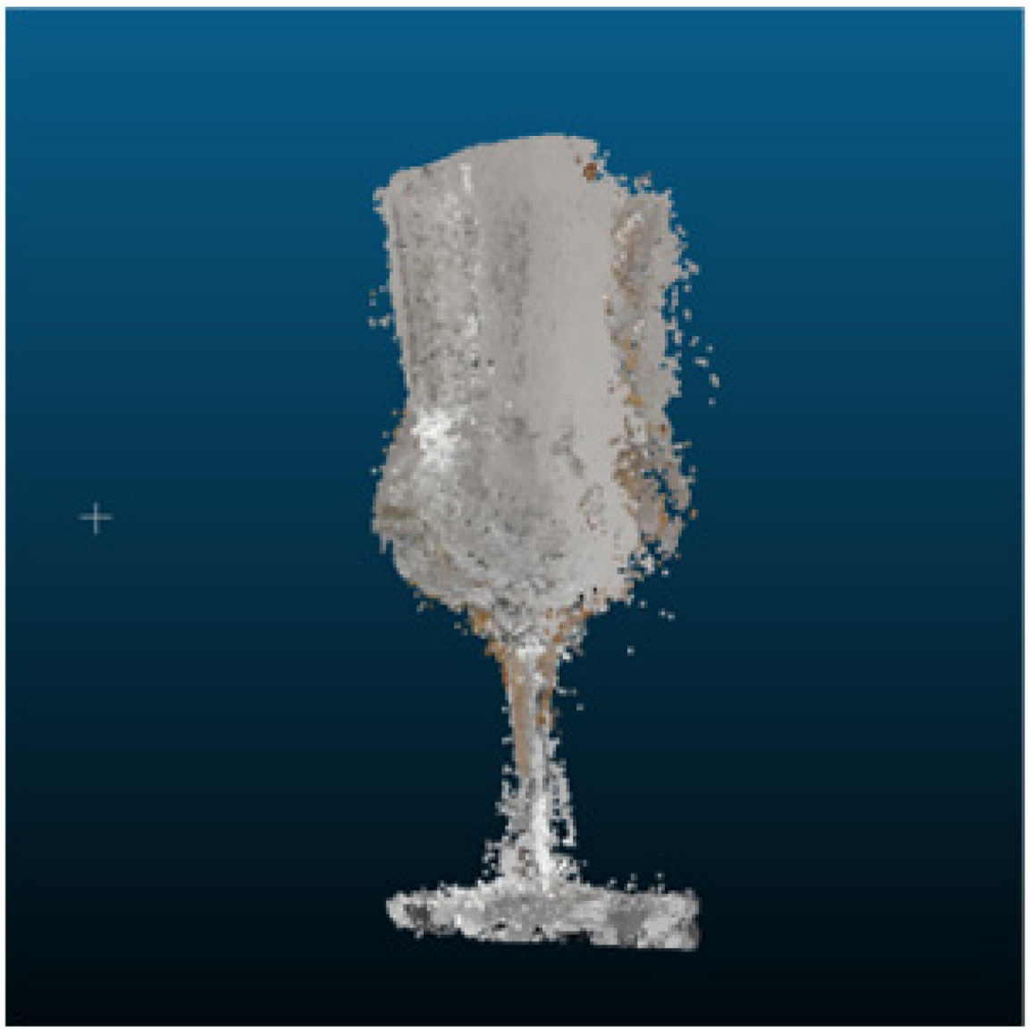 |  | 8.17 | 5.16 | 6.33 | 4.61 |
| DI-MVS |  | 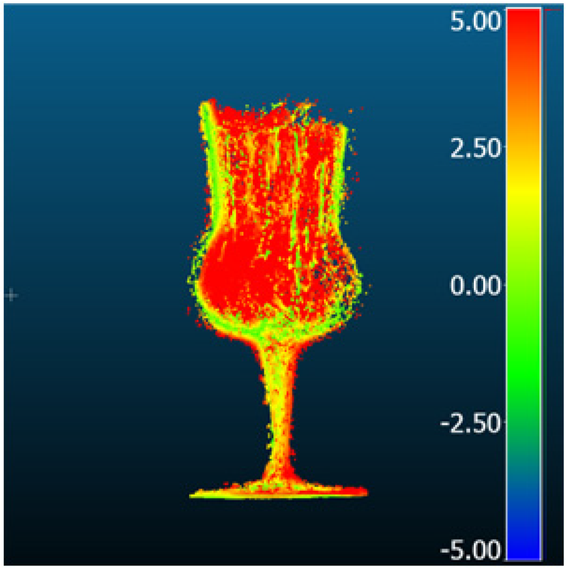 | 6.06 | 3.44 | 4.98 | 2.72 |
| KD-MVS | 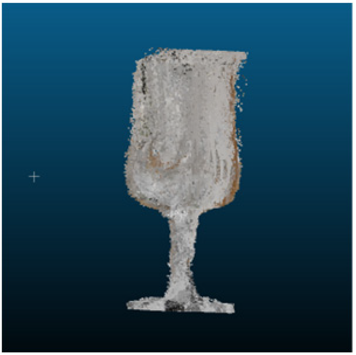 | 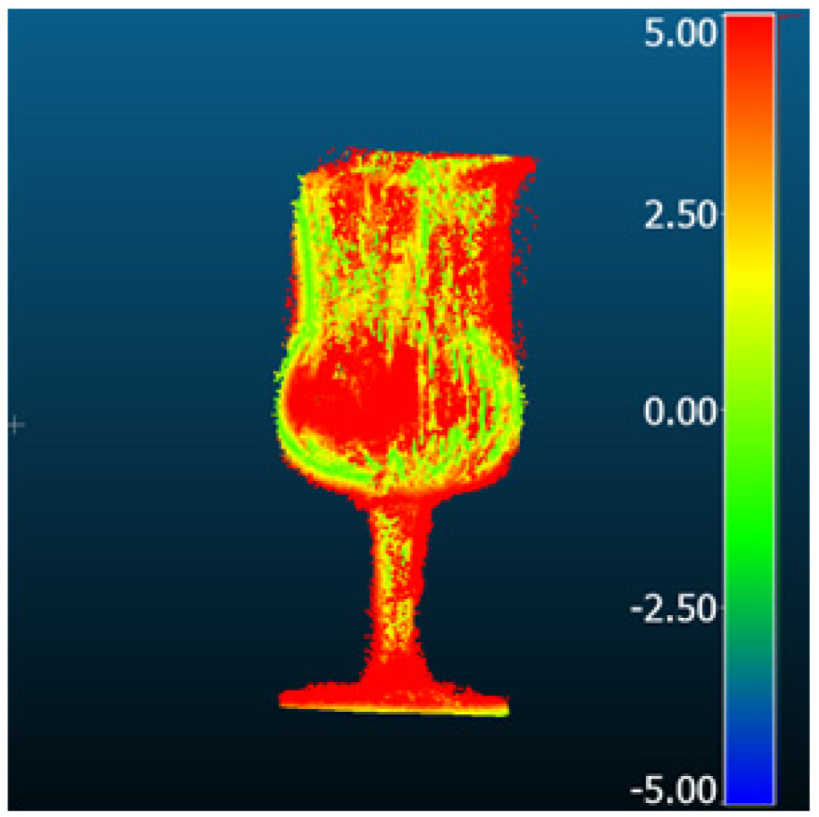 | 3.33 | 2.49 | 2.20 | 1.62 |
| MVSFormer | 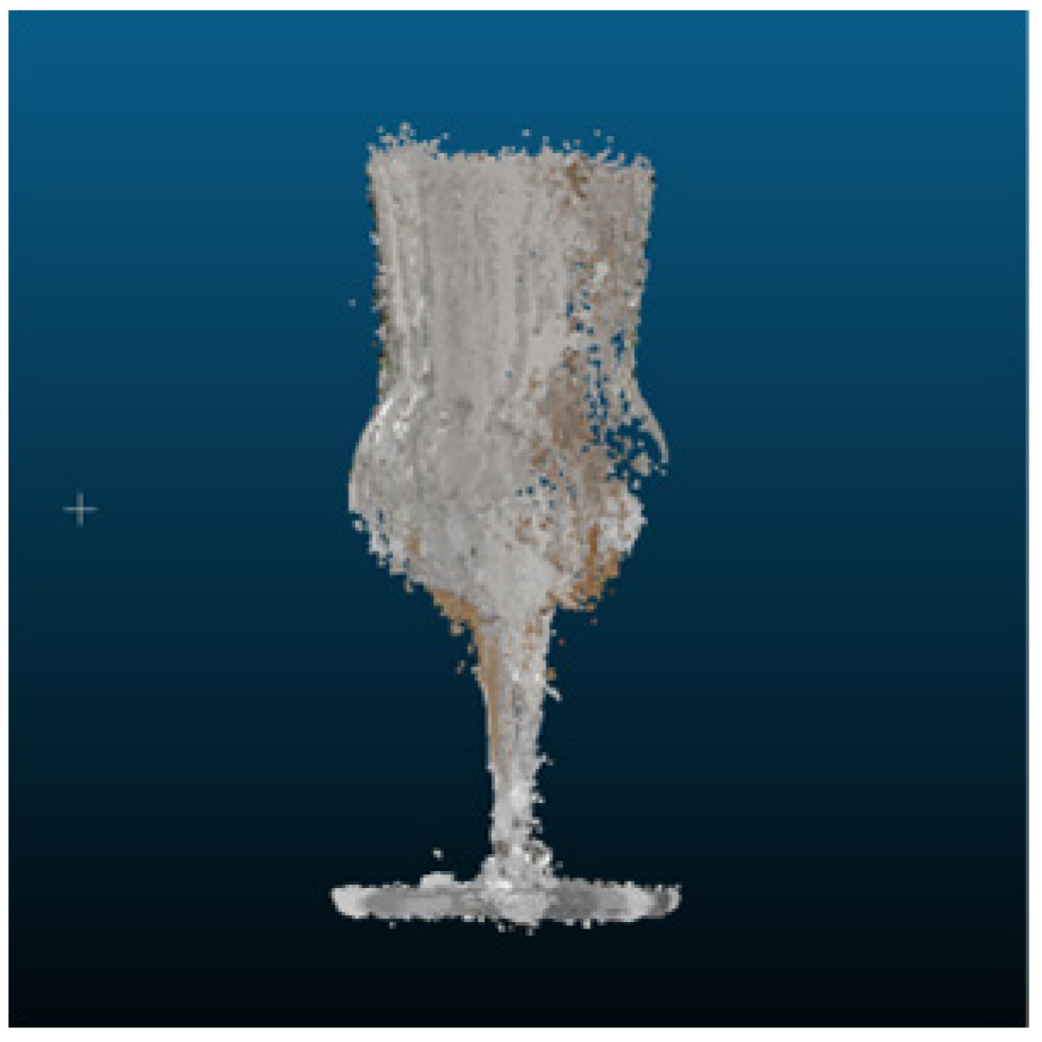 |  | 5.82 | 3.99 | 4.24 | 3.62 |
| Method | 3D Geometry | Comparison Result [mm] | Metric [mm] | |||
|---|---|---|---|---|---|---|
| RMSD | MAE | STD | Mean_E | |||
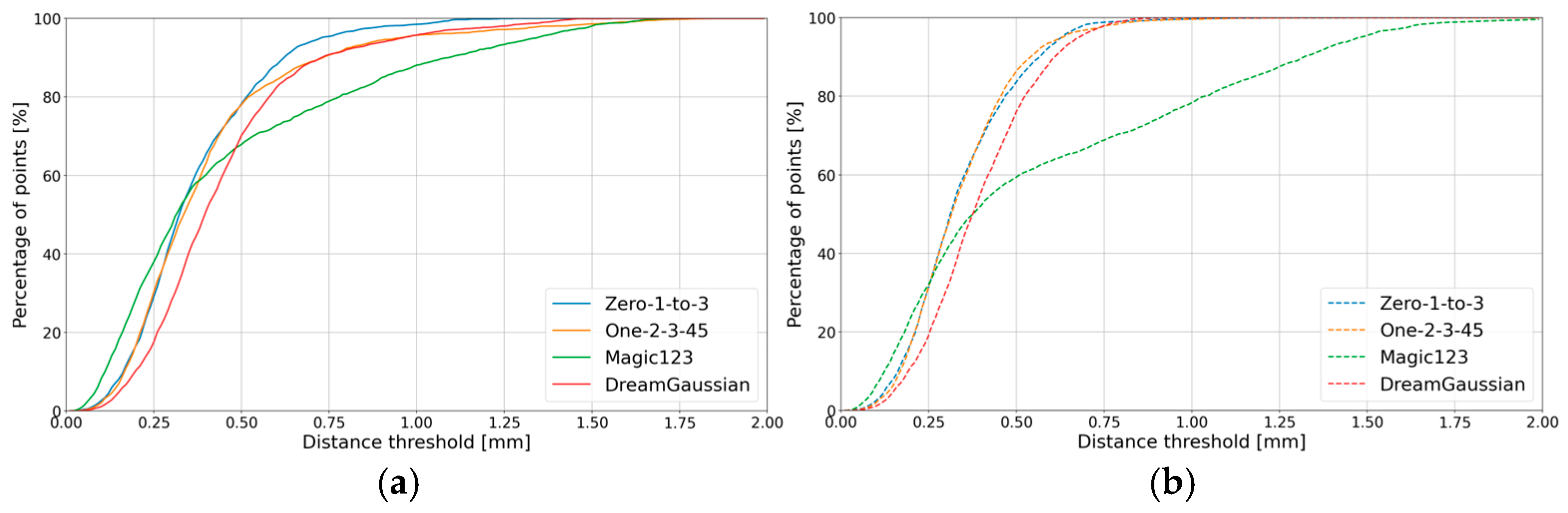
| DreamGaussian |  | 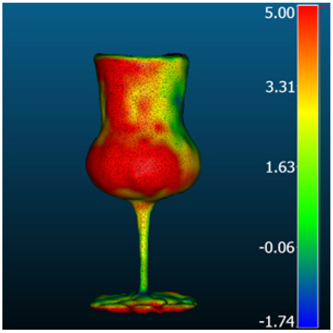 | 6.26 | 4.59 | 4.25 | 4.17 |
| Magic1233 | 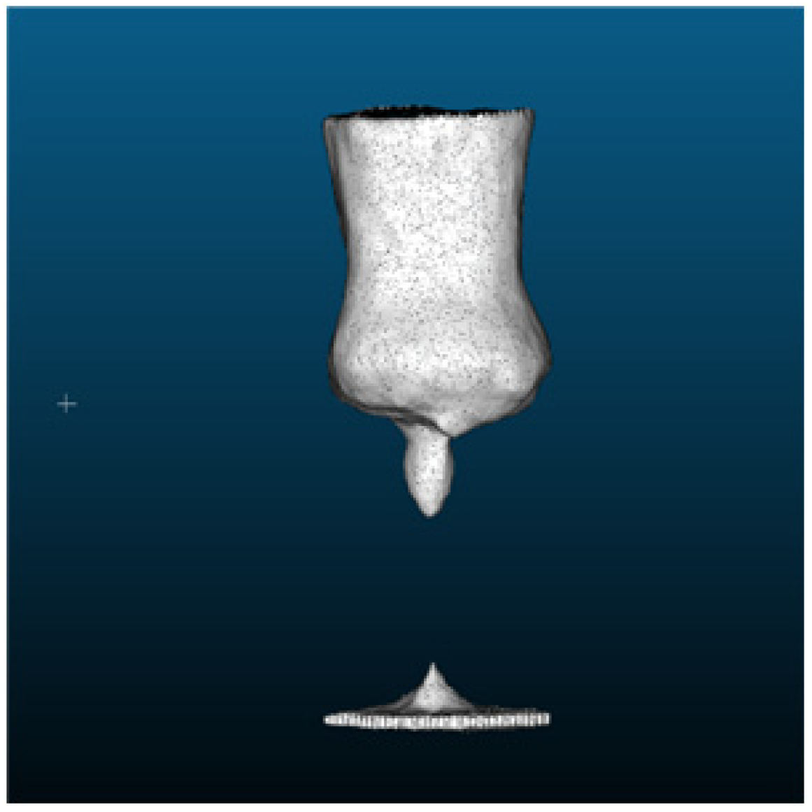 | 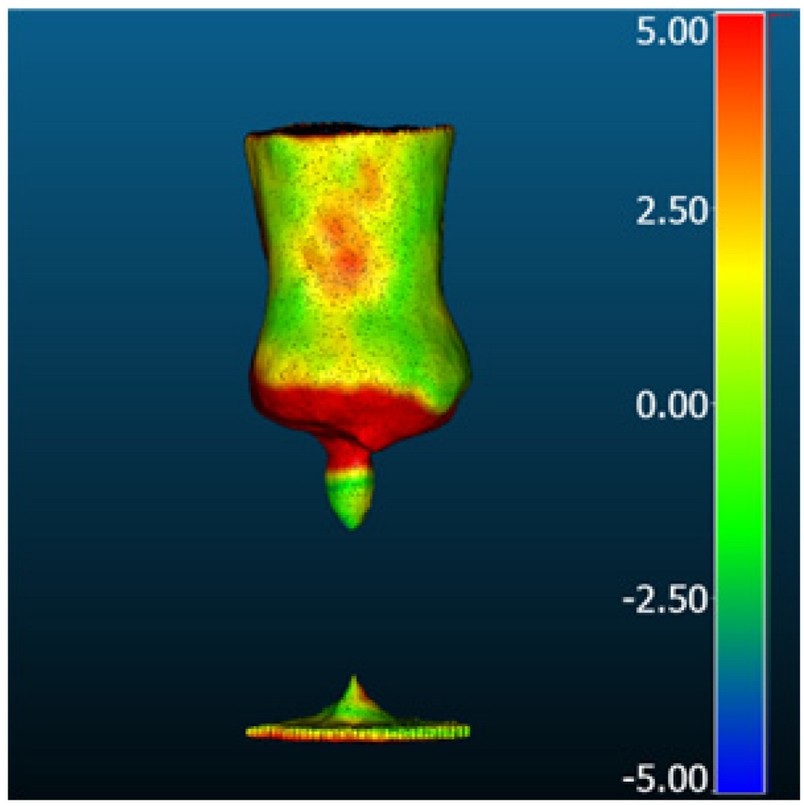 | 4.12 | 3.42 | 2.30 | 3.16 |
| One-2-3-45 |  | 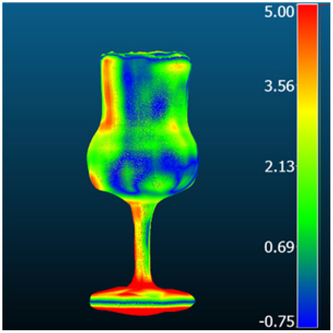 | 3.52 | 2.79 | 2.15 | 2.48 |
| Zero-1-to-3 |  |  | 3.32 | 2.76 | 1.85 | 2.39 |
References
- Li, Q.; Huang, H.; Yu, W.; Jiang, S. Optimized views photogrammetry: Precision analysis and a large-scale case study in qingdao. IEEE J. Sel. Top. Appl. Earth Obs. Remote Sens. 2023, 16, 1144–1159. [Google Scholar]
- Hosseininaveh, A.; Yazdan, R.; Karami, A.; Moradi, M.; Ghorbani, F. A low-cost and portable system for 3D reconstruction of texture-less objects. Int. Arch. Photogramm. Remote Sens. Spat. Inf. Sci. 2015, 40, 327–332. [Google Scholar]
- Ahmadabadian, A.H.; Karami, A.; Yazdan, R. An automatic 3D reconstruction system for texture-less objects. Robot. Auton. Syst. 2019, 117, 29–39. [Google Scholar] [CrossRef]
- Menna, F.; Nocerino, E.; Morabito, D.; Farella, E.M.; Perini, M.; Remondino, F. An open source low-cost automatic system for image-based 3D digitization. Int. Arch. Photogramm. Remote Sens. Spat. Inf. Sci. 2017, 42, 155–162. [Google Scholar]
- Hu, Y.; Wang, S.; Cheng, X.; Xu, C.; Hao, Q. Dynamic deformation measurement of specular surface with deflectometry and speckle digital image correlation. Sensors 2020, 20, 1278. [Google Scholar] [CrossRef]
- Parras-Burgos, D.; Fernández-Pacheco, D.G.; Cavas-Martínez, F.; Nieto, J.; Cañavate, F.J. Initiation to Reverse Engineering by Using Activities Based on Photogrammetry as New Teaching Method in University Technical Studies. In Proceedings of the 13th UAHCI, Orlando, FL, USA, 26 July 2019; Volume 21, pp. 159–176. [Google Scholar]
- Huang, S.; Xu, K.; Li, M.; Wu, M. Improved visual inspection through 3D image reconstruction of defects based on the photometric stereo technique. Sensors 2019, 19, 4970. [Google Scholar] [CrossRef] [PubMed]
- Karami, A.; Menna, F.; Remondino, F. Investigating 3D reconstruction of non-collaborative surfaces through photogrammetry and photometric stereo. Int. Arch. Photogramm. Remote Sens. Spat. Inf. Sci. 2021, 43, 519–526. [Google Scholar] [CrossRef]
- Lu, Z.; Cai, L. Accurate three-dimensional measurement for small objects based on the thin-lens model. Appl. Opt. 2020, 59, 6600–6611. [Google Scholar] [CrossRef]
- Anciukevičius, T.; Xu, Z.; Fisher, M.; Henderson, P.; Bilen, H.; Mitra, N.J.; Guerrero, P. Renderdiffusion: Image diffusion for 3D reconstruction, inpainting and generation. In Proceedings of the IEEE/CVF Conference on Computer Vision and Pattern Recognition, Vancouver, BC, Canada, 17–24 June 2023; pp. 12608–12618. [Google Scholar]
- Hafeez, J.; Lee, J.; Kwon, S.; Ha, S.; Hur, G.; Lee, S. Evaluating feature extraction methods with synthetic noise patterns for image-based modelling of texture-less objects. Remote Sens. 2020, 12, 3886. [Google Scholar] [CrossRef]
- Morelli, L.; Karami, A.; Menna, F.; Remondino, F. Orientation of images with low contrast textures and transparent objects. Int. Arch. Photogramm. Remote Sens. Spat. Inf. Sci 2022, 48, 77–84. [Google Scholar]
- Gao, K.; Gao, Y.; He, H.; Lu, D.; Xu, L.; Li, J. Nerf: Neural radiance field in 3D vision, a comprehensive review. arXiv 2022, arXiv:2210.00379. [Google Scholar]
- Remondino, F.; Karami, A.; Yan, Z.; Mazzacca, G.; Rigon, S.; Qin, R. A critical analysis of nerf-based 3D reconstruction. Remote Sens. 2023, 15, 3585. [Google Scholar]
- Stathopoulou, E.K.; Remondino, F. A survey on conventional and learning-based methods for multi-view stereo. Photogramm. Rec. 2023, 38, 374–407. [Google Scholar]
- Yin, W.; Zhang, C.; Chen, H.; Cai, Z.; Yu, G.; Wang, K.; Chen, X.; Shen, C. Metric3D: Towards zero-shot metric 3D prediction from a single image. In Proceedings of the IEEE/CVF International Conference on Computer Vision, Vancouver, BC, Canada, 1–6 October 2023; pp. 9043–9053. [Google Scholar]
- Yan, Z.; Mazzacca, G.; Rigon, S.; Farella, E.M.; Trybala, P.; Remondino, F. NeRFBK: A holistic dataset for benchmarking NeRF-based 3D reconstruction. ISPRS Int. Arch. Photogramm. Remote Sens. Spat. Inf. Sci. 2023, 48, 219–226. [Google Scholar]
- Cline, H.E.; Dumoulin, C.L.; Hart, H.R., Jr.; Lorensen, W.E.; Ludke, S. 3D reconstruction of the brain from magnetic resonance images using a connectivity algorithm. Magn. Reson. Imaging 1987, 5, 345–352. [Google Scholar]
- Mildnhall, B.; Srinivasan, P.P.; Tancik, M.; Barron, J.T.; Ramamoorthi, R.; Ng, R. Nerf: Representing scenes as neural radiance fields for view synthesis. Commun. ACM 2021, 65, 99–106. [Google Scholar]
- Guo, Y.C.; Kang, D.; Bao, L.; He, Y.; Zhang, S.H. Nerfren: Neural radiance fields with reflections. In Proceedings of the IEEE/CVF Conference on Computer Vision and Pattern Recognition, New Orleans, LA, USA, 17–24 June 2022; pp. 18409–18418. [Google Scholar]
- Ichnowski, J.; Avigal, Y.; Kerr, J.; Goldberg, K. Dex-NeRF: Using a neural radiance field to grasp transparent objects. In Proceedings of the 5th Conference on Robot Learning, Baltimore, MD, USA, 18–24 June 2022; Volume 164, pp. 526–536. [Google Scholar]
- Verbin, D.; Hedman, P.; Mildenhall, B.; Zickler, T.; Barron, J.T.; Srinivasan, P.P. Ref-nerf: Structured view-dependent appearance for neural radiance fields. In Proceedings of the 2022 IEEE/CVF Conference on Computer Vision and Pattern Recognition, New Orleans, LA, USA, 18–24 June 2022; pp. 5481–5490. [Google Scholar]
- Choi, C.; Kim, J.; Kim, Y.M. IBL-NeRF: Image-Based Lighting Formulation of Neural Radiance Fields. arXiv 2022, arXiv:2210.08202. [Google Scholar]
- Yu, Z.; Peng, S.; Niemeyer, M.; Sattler, T.; Geiger, A. Monosdf: Exploring monocular geometric cues for neural implicit surface reconstruction. Proc. NeurIPS 2022, 35, 25018–25032. [Google Scholar]
- Li, Z.; Müller, T.; Evans, A.; Taylor, R.H.; Unberath, M.; Liu, M.Y.; Lin, C.H. Neuralangelo: High-Fidelity Neural Surface Reconstruction. In Proceedings of the IEEE/CVF Conference on Computer Vision and Pattern Recognition, Vancouver, BC, Canada, 17–24 June 2023; pp. 8456–8465. [Google Scholar]
- Müller, T.; Evans, A.; Schied, C.; Keller, A. Instant neural graphics primitives with a multiresolution hash encoding. ACM Trans. Graph. 2022, 41, 1–15. [Google Scholar]
- Deng, K.; Liu, A.; Zhu, J.Y.; Ramanan, D. Depth-supervised nerf: Fewer views and faster training for free. In Proceedings of the IEEE/CVF Conference on Computer Vision and Pattern Recognition, New Orleans, LA, USA, 18–24 June 2022; pp. 12882–12891. [Google Scholar]
- Wang, G.; Chen, Z.; Loy, C.C.; Liu, Z. Sparsenerf: Distilling depth ranking for few-shot novel view synthesis. arXiv 2023, arXiv:2303.16196. [Google Scholar]
- Jain, A.; Tancik, M.; Abbeel, P. Putting nerf on a diet: Semantically consistent few-shot view synthesis. In Proceedings of the IEEE/CVF International Conference on Computer Vision, Montreal, BC, Canada, 11–17 October 2021; pp. 5885–5894. [Google Scholar]
- Niemeyer, M.; Barron, J.T.; Mildenhall, B.; Sajjadi, M.S.; Geiger, A.; Radwan, N. Regnerf: Regularizing neural radiance fields for view synthesis from sparse inputs. In Proceedings of the IEEE/CVF Conference on Computer Vision and Pattern Recognition, New Orleans, LA, USA, 18–24 June 2022; pp. 5480–5490. [Google Scholar]
- Kwak, M.S.; Song, J.; Kim, S. Geconerf: Few-shot neural radiance fields via geometric consistency. arXiv 2023, arXiv:2301.10941. [Google Scholar]
- Roessle, B.; Barron, J.T.; Mildenhall, B.; Srinivasan, P.P.; Nießner, M. Dense depth priors for neural radiance fields from sparse input views. In Proceedings of the IEEE/CVF Conference on Computer Vision and Pattern Recognition, New Orleans, LA, USA, 18–24 June 2022; pp. 12892–12901. [Google Scholar]
- Seo, S.; Han, D.; Chang, Y.; Kwak, N. MixNeRF: Modeling a Ray with Mixture Density for Novel View Synthesis from Sparse Inputs. In Proceedings of the IEEE/CVF Conference on Computer Vision and Pattern Recognition, Vancouver, BC, Canada, 17–24 June 2023; pp. 20659–20668. [Google Scholar]
- Yang, Z.; Yang, H.; Pan, Z.; Zhu, X.; Zhang, L. Real-time photorealistic dynamic scene representation and rendering with 4d gaussian splatting. arXiv 2023, arXiv:2310.10642. [Google Scholar]
- Somraj, N.; Soundararajan, R. ViP-NeRF: Visibility Prior for Sparse Input Neural Radiance Fields. arXiv 2023, arXiv:2305.00041. [Google Scholar]
- Somraj, N.; Karanayil, A.; Soundararajan, R. SimpleNeRF: Regularizing Sparse Input Neural Radiance Fields with Simpler Solutions. In Proceedings of the SIGGRAPH Asia 2023 Conference Papers, Sydney, NSW, Australia, 12–15 December 2023; pp. 1–11. [Google Scholar]
- Yu, A.; Ye, V.; Tancik, M.; Kanazawa, A. pixelnerf: Neural radiance fields from one or few images. In Proceedings of the IEEE/CVF Conference on Computer Vision and Pattern Recognition (CVPR), Nashville, TN, USA, 19–25 June 2021; pp. 4578–4587. [Google Scholar]
- Wynn, J.; Turmukhambetov, D. Diffusionerf: Regularizing neural radiance fields with denoising diffusion models. In Proceedings of the IEEE/CVF Conference on Computer Vision and Pattern Recognition, Vancouver, BC, Canada, 20–25 June 2023; pp. 4180–4189. [Google Scholar]
- Wu, R.; Mildenhall, B.; Henzler, P.; Park, K.; Gao, R.; Watson, D.; Holynski, A. ReconFusion: 3D Reconstruction with Diffusion Priors. arXiv 2023, arXiv:2312.02981. [Google Scholar]
- Cheng, K.; Long, X.; Yin, W.; Wang, J.; Wu, Z.; Ma, Y.; Wang, K.; Chen, X.; Chen, X. UC-NERF: Neural Radiance Field for under-calibrated multi-view cameras. arXiv 2023, arXiv:2311.16945. [Google Scholar]
- Westoby, M.J.; Brasington, J.; Glasser, N.F.; Hambrey, M.J.; Reynolds, J.M. Structure-from-Motion’photogrammetry: A low-cost, effective tool for geoscience applications. Geomorphology 2012, 179, 300–314. [Google Scholar]
- Radford, A.; Kim, J.W.; Hallacy, C.; Ramesh, A.; Goh, G.; Agarwal, S.; Sutskever, I. Learning transferable visual models from natural language supervision. In Proceedings of the International Conference on Machine Learning (PMLR), Virtually, 18–24 April 2021; pp. 8748–8763. [Google Scholar]
- Sofiiuk, K.; Petrov, I.; Barinova, O.; Konushin, A. f-brs: Rethinking backpropagating refinement for interactive segmentation. In Proceedings of the IEEE/CVF Conference on Computer Vision and Pattern Recognition, Seattle, WA, USA, 13–19 June 2020; pp. 8623–8632. [Google Scholar]
- Zwicker, M.; Pfister, H.; Van Baar, J.; Gross, M. EWA volume splatting. In Proceedings of the Visualization, San Diego, CA, USA, 19–24 October 2001; VIS’01. pp. 29–538. [Google Scholar]
- Kerbl, B.; Kopanas, G.; Leimkühler, T.; Drettakis, G. 3D Gaussian Splatting for Real-Time Radiance Field Rendering. ACM Trans. Graph. 2023, 42, 139. [Google Scholar]
- Chen, G.; Wang, W. A Survey on 3D Gaussian Splatting. arXiv 2024, arXiv:2401.03890. [Google Scholar]
- Guédon, A.; Lepetit, V. SuGaR: Surface-Aligned Gaussian Splatting for Efficient 3D Mesh Reconstruction and High-Quality Mesh Rendering. arXiv 2023, arXiv:2311.12775. [Google Scholar]
- Fei, B.; Xu, J.; Zhang, R.; Zhou, Q.; Yang, W.; He, Y. 3D Gaussian as a New Vision Era: A Survey. arXiv 2024, arXiv:2402.07181. [Google Scholar]
- Bottou, L. Large-scale machine learning with stochastic gradient descent. In Proceedings of the COMPSTAT’2010: 19th International Conference on Computational Statistics, Paris, France, 22–27 August 2010; pp. 177–186. [Google Scholar]
- Lee, B.; Lee, H.; Sun, X.; Ali, U.; Park, E. Deblurring 3D Gaussian Splatting. arXiv 2024, arXiv:2401.00834. [Google Scholar]
- Huang, L.; Bai, J.; Guo, J.; Guo, Y. GS++: Error Analyzing and Optimal Gaussian Splatting. arXiv 2024, arXiv:2402.00752. [Google Scholar]
- Feng, Y.; Feng, X.; Shang, Y.; Jiang, Y.; Yu, C.; Zong, Z.; Shao, T.; Wu, H.; Zhou, K.; Jiang, C.; et al. Gaussian Splashing: Dynamic Fluid Synthesis with Gaussian Splatting. arXiv 2024, arXiv:2401.15318. [Google Scholar]
- Fu, Y.; Liu, S.; Kulkarni, A.; Kautz, J.; Efros, A.A.; Wang, X. COLMAP-Free 3D Gaussian Splatting. arXiv 2023, arXiv:2312.07504. [Google Scholar]
- Qin, M.; Li, W.; Zhou, J.; Wang, H.; Pfister, H. LangSplat: 3D Language Gaussian Splatting. arXiv 2023, arXiv:2312.16084. [Google Scholar]
- Li, M.; Liu, S.; Zhou, H. SGS-SLAM: Semantic Gaussian Splatting For Neural Dense SLAM. arXiv 2024, arXiv:2402.03246. [Google Scholar]
- Zuo, X.; Samangouei, P.; Zhou, Y.; Di, Y.; Li, M. FMGS: Foundation Model Embedded 3D Gaussian Splatting for Holistic 3D Scene Understanding. arXiv 2024, arXiv:2401.01970. [Google Scholar]
- Gao, L.; Yang, J.; Zhang, B.T.; Sun, J.M.; Yuan, Y.J.; Fu, H.; Lai, Y.K. Mesh-based Gaussian Splatting for Real-time Large-scale Deformation. arXiv 2024, arXiv:2402.04796. [Google Scholar]
- Cheng, K.; Long, X.; Yang, K.; Yao, Y.; Yin, W.; Ma, Y.; Wang, W.; Chen, X. GaussianPro: 3D Gaussian Splatting with Progressive Propagation. arXiv 2024, arXiv:2402.14650. [Google Scholar]
- Yan, Z.; Low, W.F.; Chen, Y.; Lee, G.H. Multi-Scale 3D Gaussian Splatting for Anti-Aliased Rendering. arXiv 2023, arXiv:2311.17089. [Google Scholar]
- Chung, J.; Oh, J.; Lee, K.M. Depth-regularized optimization for 3D gaussian splatting in few-shot images. arXiv 2023, arXiv:2311.13398. [Google Scholar]
- Xiong, H.; Muttukuru, S.; Upadhyay, R.; Chari, P.; Kadambi, A. SparseGS: Real-Time 360 {\deg} Sparse View Synthesis using Gaussian Splatting. arXiv 2023, arXiv:2312.00206. [Google Scholar]
- Zhu, Z.; Fan, Z.; Jiang, Y.; Wang, Z. FSGS: Real-Time Few-shot View Synthesis using Gaussian Splatting. arXiv 2023, arXiv:2312.00451. [Google Scholar]
- Tang, J.; Ren, J.; Zhou, H.; Liu, Z.; Zeng, G. Dreamgaussian: Generative gaussian splatting for efficient 3D content creation. arXiv 2023, arXiv:2309.16653. [Google Scholar]
- Yan, Z.; Dong, W.; Shao, Y.; Lu, Y.; Haiyang, L.; Liu, J.; Wang, H.; Wang, Z.; Wang, Y.; Remondino, F.; et al. Renderworld: World model with self-supervised 3D label. arXiv 2024, arXiv:2409.11356. [Google Scholar]
- Yan, Z.; Li, L.; Shao, Y.; Chen, S.; Kai, W.; Hwang, J.N.; Zhao, H.; Remondino, F. 3DSceneEditor: Controllable 3D scene editing with gaussian splatting. arXiv 2024, arXiv:2412.01583. [Google Scholar]
- Yi, T.; Fang, J.; Wu, G.; Xie, L.; Zhang, X.; Liu, W.; Wang, X. Gaussiandreamer: Fast generation from text to 3D gaussian splatting with point cloud priors. arXiv 2023, arXiv:2310.08529. [Google Scholar]
- Yang, Z.; Gao, X.; Zhou, W.; Jiao, S.; Zhang, Y.; Jin, X. Deformable 3D gaussians for high-fidelity monocular dynamic scene reconstruction. arXiv 2023, arXiv:2309.13101. [Google Scholar]
- Huang, Y.; Cui, B.; Bai, L.; Guo, Z.; Xu, M.; Ren, H. Endo-4dgs: Distilling depth ranking for endoscopic monocular scene reconstruction with 4d gaussian splatting. arXiv 2024, arXiv:2401.16416. [Google Scholar]
- Wu, G.; Yi, T.; Fang, J.; Xie, L.; Zhang, X.; Wei, W.; Liu, W.; Tian, Q.; Wang, X. 4d gaussian splatting for real-time dynamic scene rendering. arXiv 2023, arXiv:2310.08528. [Google Scholar]
- Moreau, A.; Song, J.; Dhamo, H.; Shaw, R.; Zhou, Y.; Pérez-Pellitero, E. Human Gaussian Splatting: Real-time Rendering of Animatable Avatars. arXiv 2023, arXiv:2311.17113. [Google Scholar]
- Zielonka, W.; Bagautdinov, T.; Saito, S.; Zollhöfer, M.; Thies, J.; Romero, J. Drivable 3D gaussian avatars. arXiv 2023, arXiv:2311.08581. [Google Scholar]
- Qian, Z.; Wang, S.; Mihajlovic, M.; Geiger, A.; Tang, S. 3DGS-Avatar: Animatable Avatars via Deformable 3D Gaussian Splatting. arXiv 2023, arXiv:2312.09228. [Google Scholar]
- Dhamo, H.; Nie, Y.; Moreau, A.; Song, J.; Shaw, R.; Zhou, Y.; Pérez-Pellitero, E. HeadGaS: Real-Time Animatable Head Avatars via 3D Gaussian Splatting. arXiv 2023, arXiv:2312.02902. [Google Scholar]
- Chen, Y.; Wang, L.; Li, Q.; Xiao, H.; Zhang, S.; Yao, H.; Liu, Y. Monogaussianavatar: Monocular gaussian point-based head avatar. arXiv 2023, arXiv:2312.04558. [Google Scholar]
- Liu, Y.; Li, C.; Yang, C.; Yuan, Y. EndoGaussian: Gaussian Splatting for Deformable Surgical Scene Reconstruction. arXiv 2024, arXiv:2401.12561. [Google Scholar]
- Yan, C.; Qu, D.; Wang, D.; Xu, D.; Wang, Z.; Zhao, B.; Li, X. GS-SLAM: Dense Visual SLAM with 3D Gaussian Splatting. arXiv 2023, arXiv:2311.11700. [Google Scholar]
- Yugay, V.; Li, Y.; Gevers, T.; Oswald, M.R. Gaussian-SLAM: Photo-realistic Dense SLAM with Gaussian Splatting. arXiv 2023, arXiv:2312.10070. [Google Scholar]
- Lu, T.; Yu, M.; Xu, L.; Xiangli, Y.; Wang, L.; Lin, D.; Dai, B. Scaffold-GS: Structured 3D Gaussians for View-Adaptive Rendering. arXiv 2023, arXiv:2312.00109. [Google Scholar]
- Jiang, Y.; Tu, J.; Liu, Y.; Gao, X.; Long, X.; Wang, W.; Ma, Y. GaussianShader: 3D Gaussian Splatting with Shading Functions for Reflective Surfaces. arXiv 2023, arXiv:2311.17977. [Google Scholar]
- Tancik, M.; Weber, E.; Ng, E.; Li, R.; Yi, B.; Wang, T.; Kristoffersen, A.; Austin, J.; Salahi, K.; Ahuja, A.; et al. Nerfstudio: A modular framework for neural radiance field development. In Proceedings of the ACM SIGGRAPH 2023 Conference, Los Angeles, CA, USA, 6–10 August 2023; pp. 1–12. [Google Scholar]
- Hisham, M.B.; Yaakob, S.N.; Raof, R.A.A.; Nazren, A.A.; Wafi, N.M. Template matching using sum of squared difference and normalized cross correlation. In Proceedings of the 2015 IEEE Student Conference on Research and Development, Kuala, Malaysia, 13–14 December 2015; pp. 100–104. [Google Scholar]
- Wang, Y.; Luo, K.; Chen, Z.; Ju, L.; Guan, T. DeepFusion: A simple way to improve traditional multi-view stereo methods using deep learning. Knowl. Based Syst. 2021, 221, 106968. [Google Scholar]
- Rong, F.; Xie, D.; Zhu, W.; Shang, H.; Song, L. A survey of multi view stereo. In Proceedings of the 2021 International Conference on Networking Systems of AI, Shanghai, China, 19–20 November 2021; pp. 129–135. [Google Scholar]
- Ji, M.; Gall, J.; Zheng, H.; Liu, Y.; Fang, L. Surfacenet: An end-to-end 3D neural network for multiview stereopsis. In Proceedings of the IEEE International Conference on Computer Vision, Venice, Italy, 22–29 October 2017; pp. 2307–2315. [Google Scholar]
- Yao, Y.; Luo, Z.; Li, S.; Fang, T.; Quan, L. Mvsnet: Depth inference for unstructured multi-view stereo. In Proceedings of the European Conference on Computer Vision, Munich, Germany, 8–14 September 2018; pp. 767–783. [Google Scholar]
- Wei, Z.; Zhu, Q.; Min, C.; Chen, Y.; Wang, G. Aa-rmvsnet: Adaptive aggregation recurrent multi-view stereo network. In Proceedings of the IEEE/CVF International Conference on Computer Vision, Montreal, QC, Canada, 11–17 October 2021; pp. 6187–6196. [Google Scholar]
- Chen, R.; Han, S.; Xu, J.; Su, H. Point-based multi-view stereo network. In Proceedings of the IEEE/CVF International Conference on Computer Vision, Seoul, Republic of Korea, 27 October–2 November 2019; pp. 1538–1547. [Google Scholar]
- Luo, K.; Guan, T.; Ju, L.; Huang, H.; Luo, Y. P-mvsnet: Learning patch-wise matching confidence aggregation for multi-view stereo. In Proceedings of the IEEE/CVF International Conference on Computer Vision, Seoul, Republic of Korea, 27 October–2 November 2019; pp. 10452–10461. [Google Scholar]
- Xue, Y.; Chen, J.; Wan, W.; Huang, Y.; Yu, C.; Li, T.; Bao, J. Mvscrf: Learning multi-view stereo with conditional random fields. In Proceedings of the IEEE/CVF International Conference on Computer Vision, Seoul, Republic of Korea, 27 October–2 November 2019; pp. 4312–4321. [Google Scholar]
- Yang, J.; Mao, W.; Alvarez, J.M.; Liu, M. Cost volume pyramid based depth inference for multi-view stereo. In Proceedings of the IEEE/CVF Conference on Computer Vision and Pattern Recognition, Seattle, WA, USA, 13–19 June 2020; pp. 4877–4886. [Google Scholar]
- Yu, Z.; Gao, S. Fast-mvsnet: Sparse-to-dense multi-view stereo with learned propagation and gauss-newton refinement. In Proceedings of the IEEE/CVF Conference on Computer Vision and Pattern Recognition, Seattle, WA, USA, 13–19 June 2020; pp. 1949–1958. [Google Scholar]
- Cheng, S.; Xu, Z.; Zhu, S.; Li, Z.; Li, L.E.; Ramamoorthi, R.; Su, H. Deep stereo using adaptive thin volume representation with uncertainty awareness. In Proceedings of the IEEE/CVF Conference on Computer Vision and Pattern Recognition, Seattle, WA, USA, 13–19 June 2020; pp. 2524–2534. [Google Scholar]
- Yi, H.; Wei, Z.; Ding, M.; Zhang, R.; Chen, Y.; Wang, G.; Tai, Y.W. Pyramid multi-view stereo net with self-adaptive view aggregation. In Proceedings of the Computer Vision–ECCV 2020: 16th European Conference, Glasgow, UK, 23–28 October 2020; pp. 766–782. [Google Scholar]
- Yan, J.; Wei, Z.; Yi, H.; Ding, M.; Zhang, R.; Chen, Y.; Tai, Y.W. Dense hybrid recurrent multi-view stereo net with dynamic consistency checking. In Proceedings of the European Conference on Computer Vision (ECCV), Glasgow, UK, 23–28 October 2020; pp. 674–689. [Google Scholar]
- Zhang, J.; Li, S.; Luo, Z.; Fang, T.; Yao, Y. Vis-mvsnet: Visibility-aware multi-view stereo network. Int. J. Comput. Vis. 2023, 131, 199–214. [Google Scholar]
- Ma, X.; Gong, Y.; Wang, Q.; Huang, J.; Chen, L.; Yu, F. Epp-mvsnet: Epipolar-assembling based depth prediction for multi-view stereo. In Proceedings of the IEEE/CVF International Conference on Computer Vision, Montreal, QC, Canada, 10–17 October 2021; pp. 5732–5740. [Google Scholar]
- Kar, A.; Häne, C.; Malik, J. Learning a multi-view stereo machine. Adv. Neural Inf. Process. Syst. 2017, 30, 365–376. [Google Scholar]
- Chen, R.; Han, S.; Xu, J.; Su, H. Visibility-aware point-based multi-view stereo network. IEEE Trans. Pattern Anal. Mach. Intell. 2020, 43, 3695–3708. [Google Scholar]
- Wang, Y.; Guan, T.; Chen, Z.; Luo, Y.; Luo, K.; Ju, L. Mesh-guided multi-view stereo with pyramid architecture. In Proceedings of the IEEE/CVF Conference on Computer Vision and Pattern Recognition, Seattle, WA, USA, 13–19 June 2020; pp. 2039–2048. [Google Scholar]
- Wang, F.; Galliani, S.; Vogel, C.; Speciale, P.; Pollefeys, M. Patchmatchnet: Learned multi-view patchmatch stereo. In Proceedings of the IEEE/CVF Conference on Computer Vision and Pattern Recognition, Nashville, TN, USA, 20–25 October 2021; pp. 14194–14203. [Google Scholar]
- Xu, Q.; Tao, W. Multi-scale geometric consistency guided multi-view stereo. In Proceedings of the IEEE/CVF Conference on Computer Vision and Pattern Recognition, Long Beach, CA, USA, 15–20 October 2019; pp. 5483–5492. [Google Scholar]
- Chen, P.H.; Yang, H.C.; Chen, K.W.; Chen, Y.S. MVSNet++: Learning depth-based attention pyramid features for multi-view stereo. IEEE Trans. Image Process. 2020, 29, 7261–7273. [Google Scholar]
- Rich, A.; Stier, N.; Sen, P.; Höllerer, T. 3Dvnet: Multi-view depth prediction and volumetric refinement. In Proceedings of the 2021 International Conference on 3D Vision (3DV), Virtually, 1–3 December 2021; pp. 700–709. [Google Scholar]
- Mi, Z.; Di, C.; Xu, D. Generalized binary search network for highly-efficient multi-view stereo. In Proceedings of the IEEE/CVF Conference on Computer Vision and Pattern Recognition, New Orleans, LA, USA, 18–24 June 2022; pp. 12991–13000. [Google Scholar]
- Wang, X.; Zhu, Z.; Huang, G.; Qin, F.; Ye, Y.; He, Y.; Chi, X.; Wang, X. MVSTER: Epipolar transformer for efficient multi-view stereo. In Proceedings of the European Conference on Computer Vision, Tel Aviv, Israel, 23–27 October 2022; pp. 573–591. [Google Scholar]
- Zhang, Z.; Peng, R.; Hu, Y.; Wang, R. GeoMVSNet: Learning Multi-View Stereo With Geometry Perception. In Proceedings of the IEEE/CVF Conference on Computer Vision and Pattern Recognition, Vancouver, BC, Canada, 17–24 June 2023; pp. 21508–21518. [Google Scholar]
- Eigen, D.; Puhrsch, C.; Fergus, R. Depth map prediction from a single image using a multi-scale deep network. Adv. Neural Inf. Process. Syst. 2014, 27. [Google Scholar]
- Laina, I.; Rupprecht, C.; Belagiannis, V.; Tombari, F.; Navab, N. Deeper depth prediction with fully convolutional residual networks. In Proceedings of the 2016 Fourth international conference on 3D vision (3DV), Stanford, CA, USA, 25–28 October 2016; pp. 239–248. [Google Scholar]
- Yang, G.; Tang, H.; Ding, M.; Sebe, N.; Ricci, E. Transformer-based attention networks for continuous pixel-wise prediction. In Proceedings of the IEEE/CVF International Conference on Computer Vision, Montreal, QC, Canada, 11–17 October 2021; pp. 16269–16279. [Google Scholar]
- Ranftl, R.; Bochkovskiy, A.; Koltun, V. Vision transformers for dense prediction. In Proceedings of the IEEE/CVF International Conference on Computer Vision, Montreal, QC, Canada, 11–17 October 2021; pp. 12179–12188. [Google Scholar]
- Yuan, W.; Gu, X.; Dai, Z.; Zhu, S.; Tan, P. Neural window fully-connected crfs for monocular depth estimation. In Proceedings of the IEEE/CVF Conference on Computer Vision and Pattern Recognition, New Orleans, LA, USA, 18–24 June 2022; pp. 3916–3925. [Google Scholar]
- Shao, S.; Pei, Z.; Wu, X.; Liu, Z.; Chen, W.; Li, Z. IEBins: Iterative elastic bins for monocular depth estimation. Adv. Neural Inf. Process. Syst. 2024, 36, 53025–53037. [Google Scholar]
- Ming, Y.; Meng, X.; Fan, C.; Yu, H. Deep learning for monocular depth estimation: A review. Neurocomputing 2021, 438, 14–33. [Google Scholar]
- Fu, H.; Gong, M.; Wang, C.; Batmanghelich, K.; Tao, D. Deep ordinal regression network for monocular depth estimation. In Proceedings of the IEEE Conference on Computer Vision and Pattern Recognition, Salt Lake City, UT, USA, 18–23 June 2018; pp. 2002–2011. [Google Scholar]
- Facil, J.M.; Ummenhofer, B.; Zhou, H.; Montesano, L.; Brox, T.; Civera, J. CAM-Convs: Camera-aware multi-scale convolutions for single-view depth. In Proceedings of the IEEE/CVF Conference on Computer Vision and Pattern Recognition, Long Beach, CA, USA, 13–19 June 2019; pp. 11826–11835. [Google Scholar]
- Wofk, D.; Ma, F.; Yang, T.J.; Karaman, S.; Sze, V. Fastdepth: Fast monocular depth estimation on embedded systems. In Proceedings of the 2019 International Conference on Robotics and Automation, Montreal, QC, Canada, 15–20 May 2019; pp. 6101–6108. [Google Scholar]
- Zhao, S.; Fu, H.; Gong, M.; Tao, D. Geometry-aware symmetric domain adaptation for monocular depth estimation. In Proceedings of the IEEE/CVF Conference on Computer Vision and Pattern Recognition, Long Beach, CA, USA, 15–20 June 2019; pp. 9788–9798. [Google Scholar]
- Wu, Z.; Wu, X.; Zhang, X.; Wang, S.; Ju, L. Spatial correspondence with generative adversarial network: Learning depth from monocular videos. In Proceedings of the IEEE/CVF International Conference on Computer Vision, Seoul, Republic of Korea, 27 October–2 November 2019; pp. 7494–7504. [Google Scholar]
- Wimbauer, F.; Yang, N.; Von Stumberg, L.; Zeller, N.; Cremers, D. MonoRec: Semi-supervised dense reconstruction in dynamic environments from a single moving camera. In Proceedings of the IEEE/CVF Conference on Computer Vision and Pattern Recognition, Nashville, TN, USA, 20–25 June 2021; pp. 6112–6122. [Google Scholar]
- Zhang, N.; Nex, F.; Vosselman, G.; Kerle, N. Lite-mono: A lightweight cnn and transformer architecture for self-supervised monocular depth estimation. In Proceedings of the IEEE/CVF Conference on Computer Vision and Pattern Recognition, Vancouver, BC, Canada, 17–24 June 2023; pp. 18537–18546. [Google Scholar]
- Bhoi, A. Monocular depth estimation: A survey. arXiv 2019, arXiv:1901.09402. [Google Scholar]
- Garg, R.; Bg, V.K.; Carneiro, G.; Reid, I. Unsupervised cnn for single view depth estimation: Geometry to the rescue. In Proceedings of the Computer Vision–ECCV 2016: 14th European Conference, Amsterdam, The Netherlands, 11–14 October 2016; Part VIII 14. pp. 740–756. [Google Scholar]
- Godard, C.; Mac Aodha, O.; Brostow, G.J. Unsupervised monocular depth estimation with left-right consistency. In Proceedings of the IEEE Conference on Computer Vision and Pattern Recognition, Honolulu, HI, USA, 21–26 June 2017; pp. 270–279. [Google Scholar]
- Zhou, T.; Brown, M.; Snavely, N.; Lowe, D.G. Unsupervised learning of depth and ego-motion from video. In Proceedings of the IEEE Conference on Computer Vision and Pattern Recognition, Honolulu, HI, USA, 21–26 June 2017; pp. 1851–1858. [Google Scholar]
- Flynn, J.; Neulander, I.; Philbin, J.; Snavely, N. Deepstereo: Learning to predict new views from the world’s imagery. In Proceedings of the IEEE Conference on Computer Vision and Pattern Recognition, Las Vegas, NV, USA, 27–30 June 2016; pp. 5515–5524. [Google Scholar]
- Bhat, S.F.; Birkl, R.; Wofk, D.; Wonka, P.; Müller, M. Zoedepth: Zero-shot transfer by combining relative and metric depth. arXiv 2023, arXiv:2302.1228. [Google Scholar]
- Silberman, N.; Hoiem, D.; Kohli, P.; Fergus, R. Indoor segmentation and support inference from RGBd images. In Proceedings of the Computer Vision–ECCV 2012: 12th European Conference on Computer Vision, Florence, Italy, 7–13 October 2012; Volume 12, pp. 746–760. [Google Scholar]
- Menze, M.; Geiger, A. Object scene flow for autonomous vehicles. In Proceedings of the IEEE Conference on Computer Vision and Pattern Recognition, Boston, MA, USA, 7–12 June 2015; pp. 3061–3070. [Google Scholar]
- Ranftl, R.; Lasinger, K.; Hafner, D.; Schindler, K.; Koltun, V. Towards robust monocular depth estimation: Mixing datasets for zero-shot cross-dataset transfer. IEEE Trans. Pattern Anal. Mach. Intell. 2020, 44, 1623–1637. [Google Scholar]
- Birkl, R.; Wofk, D.; Müller, M. MiDaS v3. 1--A Model Zoo for Robust Monocular Relative Depth Estimation. arXiv 2023, arXiv:2307.14460. [Google Scholar]
- Yang, L.; Kang, B.; Huang, Z.; Xu, X.; Feng, J.; Zhao, H. Depth anything: Unleashing the power of large-scale unlabeled data. arXiv 2024, arXiv:2401.10891. [Google Scholar]
- Zhang, L.; Rao, A.; Agrawala, M. Adding conditional control to text-to-image diffusion models. In Proceedings of the IEEE/CVF International Conference on Computer Vision, Paris, France, 1–6 October 2023; pp. 3836–3847. [Google Scholar]
- Gu, S.; Chen, D.; Bao, J.; Wen, F.; Zhang, B.; Chen, D.; Lu, Y.; Guo, B. Vector quantized diffusion model for text-to-image synthesis. In Proceedings of the IEEE/CVF Conference on Computer Vision and Pattern Recognition, New Orleans, LA, USA, 18–24 June 2022; pp. 10696–10706. [Google Scholar]
- Ruiz, N.; Li, Y.; Jampani, V.; Pritch, Y.; Rubinstein, M.; Aberman, K. Dreambooth: Fine tuning text-to-image diffusion models for subject-driven generation. In Proceedings of the IEEE/CVF Conference on Computer Vision and Pattern Recognition, Vancouver, BC, Canada, 17–24 June 2023; pp. 22500–22510. [Google Scholar]
- Xu, Z.; Xing, S.; Sangineto, E.; Sebe, N. SpectralCLIP: Preventing Artifacts in Text-Guided Style Transfer from a Spectral Perspective. In Proceedings of the Winter Conference on Applications of Computer Vision, Waikoloa, HI, USA, 3–8 February 2024; pp. 5121–5130. [Google Scholar]
- Liao, M.; Dong, H.B.; Wang, X.; Yan, Z.; Shao, Y. GM-MoE: Low-Light Enhancement with Gated-Mechanism Mixture-of-Experts. arXiv 2025, arXiv:2503.07417. [Google Scholar]
- Esser, P.; Chiu, J.; Atighehchian, P.; Granskog, J.; Germanidis, A. Structure and content-guided video synthesis with diffusion models. In Proceedings of the IEEE/CVF International Conference on Computer Vision, Paris, France, 1–6 October 2023; pp. 7346–7356. [Google Scholar]
- Blattmann, A.; Rombach, R.; Ling, H.; Dockhorn, T.; Kim, S.W.; Fidler, S.; Kreis, K. Align your latents: High-resolution video synthesis with latent diffusion models. In Proceedings of the IEEE/CVF Conference on Computer Vision and Pattern Recognition, Vancouver, BC, Canada, 17–24 June 2023; pp. 22563–22575. [Google Scholar]
- Khachatryan, L.; Movsisyan, A.; Tadevosyan, V.; Henschel, R.; Wang, Z.; Navasardyan, S.; Shi, H. Text2video-zero: Text-to-image diffusion models are zero-shot video generators. arXiv 2023, arXiv:2303.13439. [Google Scholar]
- Ge, S.; Nah, S.; Liu, G.; Poon, T.; Tao, A.; Catanzaro, B.; Jacobs, D.; Huang, J.-B.; Liu, M.-Y.; Balaji, Y. Preserve your own correlation: A noise prior for video diffusion models. In Proceedings of the IEEE/CVF International Conference on Computer Vision, Paris, France, 4–6 October 2023; pp. 22930–22941. [Google Scholar]
- Luo, Z.; Chen, D.; Zhang, Y.; Huang, Y.; Wang, L.; Shen, Y.; Tan, T. VideoFusion: Decomposed Diffusion Models for High-Quality Video Generation. arXiv 2023, arXiv:2303.08320. [Google Scholar]
- Shao, Y.; Lin, D.; Zeng, F.; Yan, M.; Zhang, M.; Chen, S.; Fan, Y.; Yan, Z.; Wang, H.; Guo, J.; et al. TR-DQ: Time-Rotation Diffusion Quantization. arXiv 2025, arXiv:2503.06564. [Google Scholar]
- Kim, G.; Chun, S.Y. Datid-3D: Diversity-preserved domain adaptation using text-to-image diffusion for 3D generative model. In Proceedings of the IEEE/CVF Conference on Computer Vision and Pattern Recognition, Vancouver, BC, Canada, 17–24 June 2023; pp. 14203–14213. [Google Scholar]
- Ding, L.; Dong, S.; Huang, Z.; Wang, Z.; Zhang, Y.; Gong, K.; Xu, D.; Xue, T. Text-to-3D Generation with Bidirectional Diffusion using both 2D and 3D priors. arXiv 2023, arXiv:2312.04963. [Google Scholar]
- Poole, B.; Jain, A.; Barron, J.T.; Mildenhall, B. Dreamfusion: Text-to-3D using 2d diffusion. arXiv 2022, arXiv:2209.14988. [Google Scholar]
- Fang, C.; Hu, X.; Luo, K.; Tan, P. Ctrl-Room: Controllable Text-to-3D Room Meshes Generation with Layout Constraints. arXiv 2023, arXiv:2310.03602. [Google Scholar]
- Liu, M.; Shi, R.; Chen, L.; Zhang, Z.; Xu, C.; Wei, X.; Chen, H.; Zeng, C.; Gu, J.; Su, H. One-2-3-45++: Fast single image to 3D objects with consistent multi-view generation and 3D diffusion. arXiv 2023, arXiv:2311.07885. [Google Scholar]
- Long, X.; Guo, Y.C.; Lin, C.; Liu, Y.; Dou, Z.; Liu, L.; Ma, Y.; Zhang, S.-H.; Habermann, M.; Theobalt, C.; et al. Wonder3D: Single image to 3D using cross-domain diffusion. arXiv 2023, arXiv:2310.15008. [Google Scholar]
- Qian, G.; Mai, J.; Hamdi, A.; Ren, J.; Siarohin, A.; Li, B.; Ghanem, B. Magic123: One image to high-quality 3D object generation using both 2d and 3D diffusion priors. arXiv 2023, arXiv:2306.17843. [Google Scholar]
- He, L.; Yan, H.; Luo, M.; Luo, K.; Wang, W.; Du, W.; Chen, H.; Yang, H.; Zhang, Y. Iterative reconstruction based on latent diffusion model for sparse data reconstruction. arXiv 2023, arXiv:2307.12070. [Google Scholar]
- Yu, C.; Zhou, Q.; Li, J.; Zhang, Z.; Wang, Z.; Wang, F. Points-to-3D: Bridging the gap between sparse points and shape-controllable text-to-3D generation. In Proceedings of the 31st ACM International Conference on Multimedia, Ottawa, ON, Canada, 29 October–3 November; pp. 6841–6850.
- Liu, M.; Shi, R.; Kuang, K.; Zhu, Y.; Li, X.; Han, S.; Su, H. Openshape: Scaling up 3D shape representation towards open-world understanding. Adv. Neural Inf. Process. Syst. 2024, 36, 44860–44879. [Google Scholar]
- Chang, A.X.; Funkhouser, T.; Guibas, L.; Hanrahan, P.; Huang, Q.; Li, Z.; Savarese, S.; Savva, M.; Song, S.; Su, H.; et al. Shapenet: An information-rich 3D model repository. arXiv 2015, arXiv:1512.03012. [Google Scholar]
- Liu, M.; Sheng, L.; Yang, S.; Shao, J.; Hu, S.M. Morphing and sampling network for dense point cloud completion. In Proceedings of the AAAI Conference on Artificial Intelligence, New York, NY, USA, 7–8 February 2020; Volume 34, pp. 11596–11603. [Google Scholar]
- Liu, M.; Sung, M.; Mech, R.; Su, H. Deepmetahandles: Learning deformation meta-handles of 3D meshes with biharmonic coordinates. In Proceedings of the IEEE/CVF Conference on Computer Vision and Pattern Recognition, Nashville, TN, USA, 20–25 June 2021; pp. 12–21. [Google Scholar]
- Huang, Z.; Stojanov, S.; Thai, A.; Jampani, V.; Rehg, J.M. Planes vs. chairs: Category-guided 3D shape learning without any 3D cues. In Proceedings of the European Conference on Computer Vision, Tel Aviv, Israel, 23–27 October 2022; Springer Nature: Cham, Switzerland, 2022; pp. 727–744. [Google Scholar]
- Xu, J.; Wang, X.; Cheng, W.; Cao, Y.P.; Shan, Y.; Qie, X.; Gao, S. Dream3D: Zero-shot text-to-3D synthesis using 3D shape prior and text-to-image diffusion models. In Proceedings of the IEEE/CVF Conference on Computer Vision and Pattern Recognition, Vancouver, BC, Canada, 17–24 June 2023; pp. 20908–20918. [Google Scholar]
- Vincent, P.; Larochelle, H.; Bengio, Y.; Manzagol, P.A. Extracting and composing robust features with denoising autoencoders. In Proceedings of the 25th International Conference on Machine Learning, Helsinki, Finland, 5–9 July 2008; pp. 1096–1103. [Google Scholar]
- Hyvärinen, A.; Dayan, P. Estimation of non-normalized statistical models by score matching. J. Mach. Learn. Res. 2005, 6, 695–709. [Google Scholar]
- Norris, J.R. Markov Chains; Cambridge University Press: Cambridge, UK, 1998. [Google Scholar]
- Ho, J.; Jain, A.; Abbeel, P. Denoising diffusion probabilistic models. Adv. Neural Inf. Process. Syst. 2020, 33, 6840–6851. [Google Scholar]
- Du, Y.; Mordatch, I. Implicit generation and modeling with energy based models. In Proceedings of the 33rd Conference on Neural Information Processing Systems (NeurIPS): Annual Conference on Neural Information Processing Systems 2020, NeurIPS 2020, Vancouver, BC, Canada, 6–12 December 2020; pp. 3603–3613. [Google Scholar]
- Liu, R.; Wu, R.; Van Hoorick, B.; Tokmakov, P.; Zakharov, S.; Vondrick, C. Zero-1-to-3: Zero-shot one image to 3D object. In Proceedings of the IEEE/CVF International Conference on Computer Vision, Paris, France, 1–6 October 2023; pp. 9298–9309. [Google Scholar]
- Rombach, R.; Blattmann, A.; Lorenz, D.; Esser, P.; Ommer, B. High-resolution image synthesis with latent diffusion models. In Proceedings of the IEEE/CVF Conference on Computer Vision and Pattern Recognition, New Orleans, LA, USA, 18–24 June 2022; pp. 10684–10695. [Google Scholar]
- Shi, Y.; Wang, P.; Ye, J.; Long, M.; Li, K.; Yang, X. Mvdream: Multi-view diffusion for 3D generation. arXiv 2023, arXiv:2308.16512. [Google Scholar]
- Liu, Y.; Lin, C.; Zeng, Z.; Long, X.; Liu, L.; Komura, T.; Wang, W. Syncdreamer: Generating multiview-consistent images from a single-view image. arXiv 2023, arXiv:2309.03453. [Google Scholar]
- Ye, J.; Wang, P.; Li, K.; Shi, Y.; Wang, H. Consistent-1-to-3: Consistent image to 3D view synthesis via geometry-aware diffusion models. arXiv 2023, arXiv:2310.03020. [Google Scholar]
- Shi, R.; Chen, H.; Zhang, Z.; Liu, M.; Xu, C.; Wei, X.; Chen, L.; Zeng, C.; Su, H. Zero123++: A single image to consistent multi-view diffusion base model. arXiv 2023, arXiv:2310.15110. [Google Scholar]
- Wang, P.; Shi, Y. ImageDream: Image-Prompt Multi-view Diffusion for 3D Generation. arXiv 2023, arXiv:2312.02201. [Google Scholar]
- Melas-Kyriazi, L.; Rupprecht, C.; Vedaldi, A. PC2: Projection-Conditioned Point Cloud Diffusion for Single-Image 3D Reconstruction. In Proceedings of the IEEE/CVF Conference on Computer Vision and Pattern Recognition, Vancouver, BC, Canada, 17–24 June 2023; pp. 12923–12932. [Google Scholar]
- Dosovitskiy, A.; Beyer, L.; Kolesnikov, A.; Weissenborn, D.; Zhai, X.; Unterthiner, T.; Dehghani, M.; Minderer, M.; Heigold, G.; Gelly, S.; et al. An image is worth 16x16 words: Transformers for image recognition at scale. arXiv 2020, arXiv:2010.11929. [Google Scholar]
- Reizenstein, J.; Shapovalov, R.; Henzler, P.; Sbordone, L.; Labatut, P.; Novotny, D. Common objects in 3D: Large-scale learning and evaluation of real-life 3D category reconstruction. In Proceedings of the IEEE/CVF International Conference on Computer Vision, Montreal, QC, Canada, 11–17 October 2021; pp. 10901–10911. [Google Scholar]
- Shao, Y.; Liang, S.; Ling, Z.; Yan, M.; Liu, H.; Chen, S.; Yan, Z.; Zhang, C.; Qin, H.; Magno, M.; et al. GWQ: Gradient-Aware Weight Quantization for Large Language Models. arXiv 2024, arXiv:2411.00850. [Google Scholar]
- Shao, Y.; Xu, Y.; Long, X.; Chen, S.; Yan, Z.; Yang, Y.; Liu, H.; Wang, Y.; Tang, H.; Lei, Z. AccidentBlip: Agent of Accident Warning based on MA-former. arXiv 2024, arXiv:2404.12149. [Google Scholar]
- Shao, Y.; Yan, M.; Liu, Y.; Chen, S.; Chen, W.; Long, X.; Yan, Z.; Li, L.; Zhang, C.; Sebe, N.; et al. In-Context Meta LoRA Generation. arXiv 2025, arXiv:2501.17635. [Google Scholar]
- Liu, T.; Hu, Y.; Wu, W.; Wang, Y.; Xu, K.; Yin, Q. Dap: Domain-aware prompt learning for vision-and-language navigation. arXiv 2023, arXiv:2311.17812. [Google Scholar]
- Yu, Z.; Dou, Z.; Long, X.; Lin, C.; Li, Z.; Liu, Y.; Wang, W. Surf-D: High-Quality Surface Generation for Arbitrary Topologies using Diffusion Models. arXiv 2023, arXiv:2311.17050. [Google Scholar]
- Chen, Y.; Pan, Y.; Li, Y.; Yao, T.; Mei, T. Control3D: Towards controllable text-to-3D generation. In Proceedings of the 31st ACM International Conference on Multimedia, Ottawa, ON, Canada, 29 October–3 November 2023; pp. 1148–1156. [Google Scholar]
- Mercier, A.; Nakhli, R.; Reddy, M.; Yasarla, R.; Cai, H.; Porikli, F.; Berger, G. HexaGen3D: StableDiffusion is just one step away from Fast and Diverse Text-to-3D Generation. arXiv 2024, arXiv:2401.07727. [Google Scholar]
- Jiang, Z.; Lu, G.; Liang, X.; Zhu, J.; Zhang, W.; Chang, X.; Xu, H. 3D-togo: Towards text-guided cross-category 3D object generation. In Proceedings of the AAAI Conference on Artificial Intelligence, Washington, DC, USA, 7–14 February 2023; Volume 37, pp. 1051–1059. [Google Scholar]
- Li, W.; Chen, R.; Chen, X.; Tan, P. Sweetdreamer: Aligning geometric priors in 2d diffusion for consistent text-to-3D. arXiv 2023, arXiv:2310.02596. [Google Scholar]
- Park, J.; Kwon, G.; Ye, J.C. ED-NeRF: Efficient Text-Guided Editing of 3D Scene using Latent Space NeRF. arXiv 2023, arXiv:2310.02712. [Google Scholar]
- Yang, H.; Chen, Y.; Pan, Y.; Yao, T.; Chen, Z.; Mei, T. 3Dstyle-diffusion: Pursuing fine-grained text-driven 3D stylization with 2d diffusion models. In Proceedings of the 31st ACM International Conference on Multimedia, Ottawa, ON, Canada, 29 October–3 November 2023; pp. 6860–6868. [Google Scholar]
- Yu, Y.; Zhu, S.; Qin, H.; Li, H. BoostDream: Efficient Refining for High-Quality Text-to-3D Generation from Multi-View Diffusion. arXiv 2024, arXiv:2401.16764. [Google Scholar]
- Chen, Z.; Wang, F.; Liu, H. Text-to-3D using gaussian splatting. arXiv 2023, arXiv:2309.16585. [Google Scholar]
- Li, X.; Wang, H.; Tseng, K.K. GaussianDiffusion: 3D Gaussian Splatting for Denoising Diffusion Probabilistic Models with Structured Noise. arXiv 2023, arXiv:2311.11221. [Google Scholar]
- Vilesov, A.; Chari, P.; Kadambi, A. Cg3D: Compositional generation for text-to-3D via gaussian splatting. arXiv 2023, arXiv:2311.17907. [Google Scholar]
- Schoenberger, J.L. Robust Methods for Accurate and Efficient 3D Modeling from Unstructured Imagery. Ph.D. Thesis, ETH Zurich, Zürich, Switzerland, 2018. [Google Scholar]
- Besl, P.J.; McKay, N.D. Method for registration of 3-D shapes. In Sensor Fusion IV: Control Paradigms and Data Structures; SPIE: Bellingham, WA, USA, 1992; Volume 1611, pp. 586–606. [Google Scholar]
- Knapitsch, A.; Park, J.; Zhou, Q.Y.; Koltun, V. Tanks and temples: Benchmarking large-scale scene reconstruction. ACM Trans. Graph. 2017, 36, 1–13. [Google Scholar]
- Nocerino, E.; Stathopoulou, E.K.; Rigon, S.; Remondino, F. Surface reconstruction assessment in photogrammetric applications. Sensors 2020, 20, 5863. [Google Scholar] [CrossRef]
- Yu, Z.; Chen, A.; Antic, B.; Peng, S.P.; Bhattacharyya, A.; Niemeyer, M.; Tang, S.; Sattler, T.; Geiger, A. SDFStudio: A Unified Framework for Surface Reconstruction. 2022. Available online: https://github.com/autonomousvision/sdfstudio (accessed on 25 June 2023).
- Wang, P.; Liu, L.; Liu, Y.; Theobalt, C.; Komura, T.; Wang, W. Neus: Learning neural implicit surfaces by volume rendering for multi-view reconstruction. arXiv 2021, arXiv:2106.10689. [Google Scholar]
- Oechsle, M.; Peng, S.; Geiger, A. Unisurf: Unifying neural implicit surfaces and radiance fields for multi-view reconstruction. In Proceedings of the IEEE/CVF International Conference on Computer Vision, Montreal, QC, Canada, 11–17 October 2021; pp. 5589–5599. [Google Scholar]
- Yariv, L.; Gu, J.; Kasten, Y.; Lipman, Y. Volume rendering of neural implicit surfaces. Adv. Neural Inf. Process. Syst. 2021, 34, 4805–4815. [Google Scholar]
- Jiang, J.; Cao, M.; Yi, J.; Li, C. DI-MVS: Learning Efficient Multi-View Stereo With Depth-Aware Iterations. In Proceedings of the ICASSP 2024-2024 IEEE International Conference on Acoustics, Speech and Signal Processing, Seoul, Republic of Korea, 14–19 April 2024; pp. 3180–3184. [Google Scholar]
- Liu, T.; Ye, X.; Zhao, W.; Pan, Z.; Shi, M.; Cao, Z. When epipolar constraint meets non-local operators in multi-view stereo. In Proceedings of the IEEE/CVF International Conference on Computer Vision, Paris, France, 4–6 October 2023; pp. 18088–18097. [Google Scholar]
- Ding, Y.; Zhu, Q.; Liu, X.; Yuan, W.; Zhang, H.; Zhang, C. Kd-mvs: Knowledge distillation based self-supervised learning for multi-view stereo. In European Conference on Computer Vision; Springer Nature: Cham, Switzerland, 2022; pp. 630–646. [Google Scholar]
- Cao, C.; Ren, X.; Fu, Y. MVSFormer: Multi-View Stereo by Learning Robust Image Features and Temperature-based Depth. arXiv 2022, arXiv:2208.02541. [Google Scholar]
- Nan, L. 2018. Available online: https://github.com/LiangliangNan/MVStudio?tab=readme-ov-file (accessed on 1 November 2023).
- Ding, Y.; Yuan, W.; Zhu, Q.; Zhang, H.; Liu, X.; Wang, Y.; Liu, X. Transmvsnet: Global context-aware multi-view stereo network with transformers. In Proceedings of the IEEE/CVF Conference on Computer Vision and Pattern Recognition, New Orleans, LA, USA, 18–24 June 2022; pp. 8585–8594. [Google Scholar]
- Zhou, Q.Y.; Park, J.; Koltun, V. Open3D: A modern library for 3D data processing. arXiv 2018, arXiv:1801.09847. [Google Scholar]
- Li, Z.; Yeh, Y.Y.; Chandraker, M. Through the looking glass: Neural 3D reconstruction of transparent shapes. In Proceedings of the IEEE/CVF Conference on Computer Vision and Pattern Recognition, Seattle, WA, USA, 13–19 June 2020; pp. 1262–1271. [Google Scholar]
- Liu, Y.; Wang, P.; Lin, C.; Long, X.; Wang, J.; Liu, L.; Kumora, T.; Wang, W. Nero: Neural geometry and brdf reconstruction of reflective objects from multiview images. ACM Trans. Graph. 2023, 42, 1–22. [Google Scholar]
- Deng, C.; Jiang, C.; Qi, C.R.; Yan, X.; Zhou, Y.; Guibas, L.; Anguelov, D. Nerdi: Single-view nerf synthesis with language-guided diffusion as general image priors. In Proceedings of the IEEE/CVF Conference on Computer Vision and Pattern Recognition, Vancouver, BC, Canada, 17–24 June 2023; pp. 20637–20647. [Google Scholar]
- Gu, J.; Trevithick, A.; Lin, K.E.; Susskind, J.M.; Theobalt, C.; Liu, L.; Ramamoorthi, R. Nerfdiff: Single-image view synthesis with nerf-guided distillation from 3D-aware diffusion. In Proceedings of the International Conference on Machine Learning, Honolulu, HI, USA, 23–29 July 2023; pp. 11808–11826. [Google Scholar]
- Song, L.; Li, Z.; Gong, X.; Chen, L.; Chen, Z.; Xu, Y.; Yuan, J. Harnessing low-frequency neural fields for few-shot view synthesis. arXiv 2023, arXiv:2303.08370. [Google Scholar]
- Parameshwara, C.M.; Hari, G.; Fermüller, C.; Sanket, N.J.; Aloimonos, Y. Diffposenet: Direct differentiable camera pose estimation. In Proceedings of the IEEE/CVF Conference on Computer Vision and Pattern Recognition, New Orleans, LA, USA, 18–24 June 2022; pp. 6845–6854. [Google Scholar]
- Wang, Z.; Wu, S.; Xie, W.; Chen, M.; Prisacariu, V.A. NeRF--: Neural radiance fields without known camera parameters. arXiv 2021, arXiv:2102.07064. [Google Scholar]
- Bian, W.; Wang, Z.; Li, K.; Bian, J.W.; Prisacariu, V.A. Nope-nerf: Optimising neural radiance field with no pose prior. In Proceedings of the IEEE/CVF Conference on Computer Vision and Pattern Recognition, Vancouver, BC, Canada, 17–24 June 2023; pp. 4160–4169. [Google Scholar]
- Wang, S.; Leroy, V.; Cabon, Y.; Chidlovskii, B.; Revaud, J. DUSt3R: Geometric 3D Vision Made Easy. arXiv 2023, arXiv:2312.14132. [Google Scholar]
- Ma, Z.; Teed, Z.; Deng, J. Multiview stereo with cascaded epipolar raft. In Proceedings of the European Conference on Computer Vision, Tel Aviv-Yafo, Israel, 23–27 October 2022; Springer Nature: Cham, Switzerland, 2022; pp. 734–750. [Google Scholar]
- Stereopsis, R.M. Accurate, dense, and robust multiview stereopsis. IEEE Trans. Pattern Anal. Mach. Intell. 2010, 32, 1362–1376. [Google Scholar]
- Chen, X.; Zhang, H.; Yu, Z.; Opipari, A.; Chadwicke Jenkins, O. Clearpose: Large-scale transparent object dataset and benchmark. In Proceedings of the Computer Vision—ECCV 2022, Tel Aviv-Yafo, Israel, 23–27 October 2022; pp. 381–396. [Google Scholar]
- Wizadwongsa, S.; Phongthawee, P.; Yenphraphai, J.; Suwajanakorn, S. Nex: Real-time view synthesis with neural basis expansion. In Proceedings of the IEEE/CVF Conference on Computer Vision and Pattern Recognition, Nashville, TN, USA, 20–25 June 2021; pp. 8534–8543. [Google Scholar]
- Sun, T.; Zhang, G.; Yang, W.; Xue, J.H.; Wang, G. TROSD: A new RBG-d dataset for transparent and reflective object segmentation in practice. IEEE Trans. Circuits Syst. Video Technol. 2023, 33, 5721–5733. [Google Scholar]
- Chen, G.; Han, K.; Wong, K.Y.K. Tom-net: Learning transparent object matting from a single image. In Proceedings of the IEEE Conference on Computer Vision and Pattern Recognition, Salt Lake City, UT, USA, 18–23 June 2018; pp. 9233–9241. [Google Scholar]
- De Roovere, P.; Moonen, S.; Michiels, N.; Wyffels, F. Dataset of industrial metal objects. arXiv 2022, arXiv:2208.04052. [Google Scholar]


| Industrial_A | Synthetic Metallic | Synthetic Glass | |
|---|---|---|---|
 |  |  | |
| Numb. images, resolution | 290 images 1280 × 720 px | 300 images 1080 × 1920 px | 300 images 1080 × 1920 px |
| Ground truth (GT) | Triangulation-based laser scanner | Synthetic data | Synthetic data |
| Characteristics | Texture-less/small and complex | Texture-less/complex/reflective | Transparent/highly refractive |
| NeRF (Section 4.2) | ||||||||||||||
|---|---|---|---|---|---|---|---|---|---|---|---|---|---|---|
| Instant-NGP [26] | Mono-Neus [192] | MonoSDF [24] | Mono-Unisurf [192] | Nerfacto [80] | ||||||||||
| Neuralangelo [25] | NeuS [193] | Nerfacto (w/depth) [80] | Nerfacto (w/o depth) [80] | Unisurf [194] | VolSDF [195] | |||||||||
| Gaussian Splatting (Section 4.2) | ||||||||||||||
| FSGS [62] | GaussianShader [79] | Gaussian Splatting [45] | Scaffold-GS [78] | |||||||||||
| Learning-based MVS (Section 4.2) | ||||||||||||||
| DI-MVS [196] | ET-MVSNet [197] | GBi-Net [104] | GeoMVSNet [106] | |||||||||||
| KD-MVS [198] | MVSFormer [199] | MVStudio [200] | TransMVSNet [201] | |||||||||||
| MDE (Section 4.3) | ||||||||||||||
| ZoeDepth [126] | MiDaS [130] | Depth Anything [131] | ||||||||||||
| Generative AI (Section 4.4) | ||||||||||||||
| One-2-3-45 [147] | DreamGaussian [63] | Magic123 [149] | Zero-1-to-3 [163] | |||||||||||
| NeRF | Learning-Based MVS | Gaussian Splatting | ||
|---|---|---|---|---|
| 3D geometry | 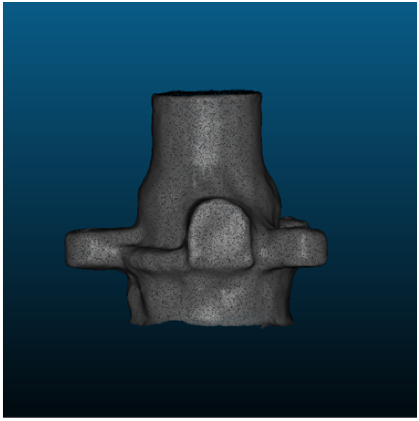 |  |  | |
| Comparison result [mm] | 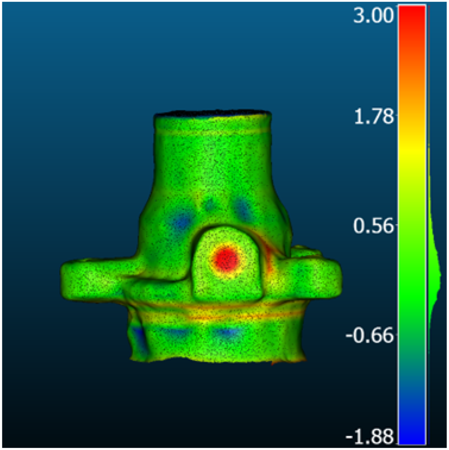 | 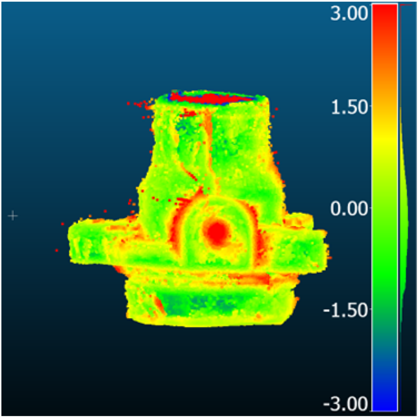 | 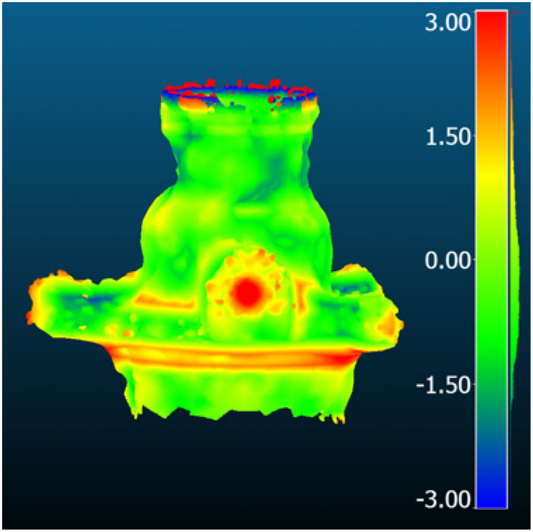 | |
| Method | Neuralangelo | MVSFormer | Gaussian Splatting | |
| Metric [mm] | RMSD | 0.57 | 0.85 | 1.11 |
| MAE | 0.43 | 0.69 | 0.89 | |
| STD | 0.37 | 0.49 | 0.66 | |
| Mean_E | 0.13 | −0.19 | 0.14 | |
| Learning-Based MVS | NeRF | Gaussian Splatting | ||
|---|---|---|---|---|
| 3D geometry | 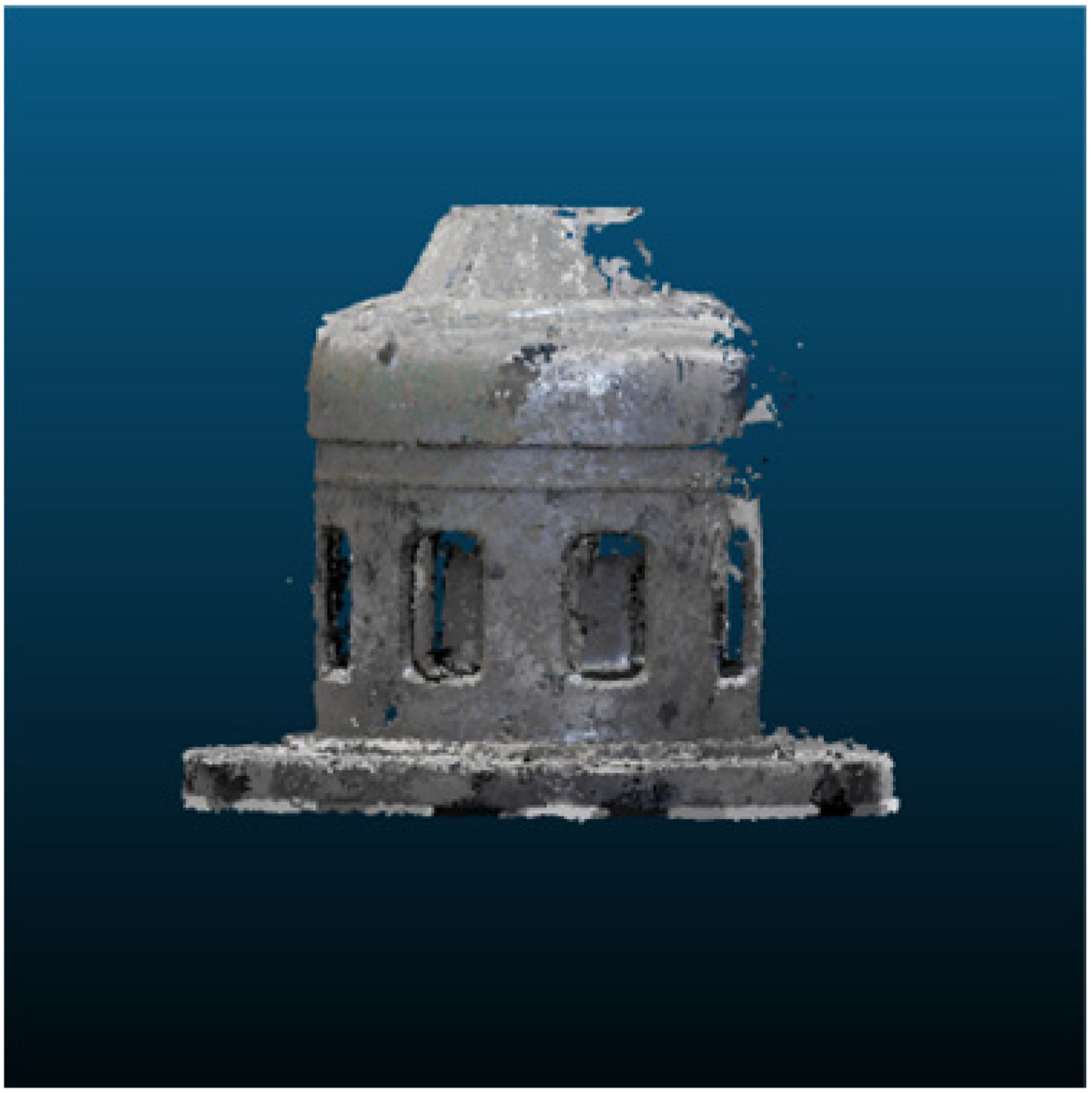 | 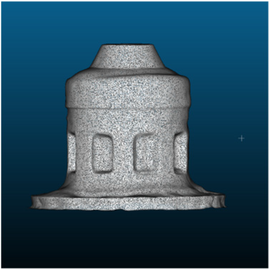 |  | |
| Comparison result [mm] | 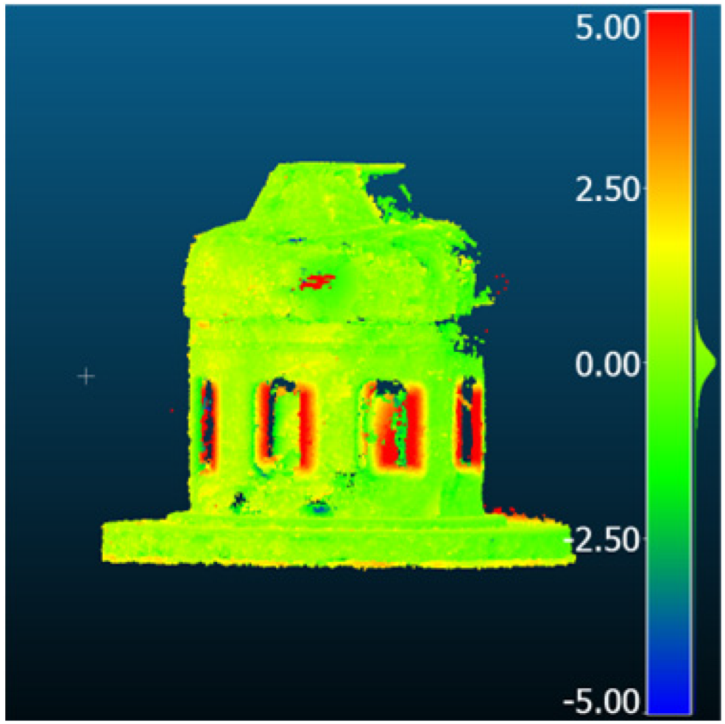 | 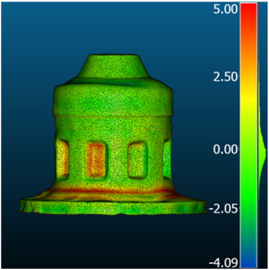 |  | |
| Method | GBi-Net | Mono-Neus | FSGS | |
| Metric [mm] | RMSD | 0.70 | 1.38 | 1.92 |
| MAE | 0.61 | 1.10 | 1.49 | |
| STD | 0.35 | 0.83 | 1.22 | |
| Mean_E | 0.00 | 0.32 | −0.41 | |
| Gaussian Splatting | NeRF | Learning-Based MVS | ||
|---|---|---|---|---|
| 3D geometry |  |  |  | |
| Comparison result [mm] |  |  | 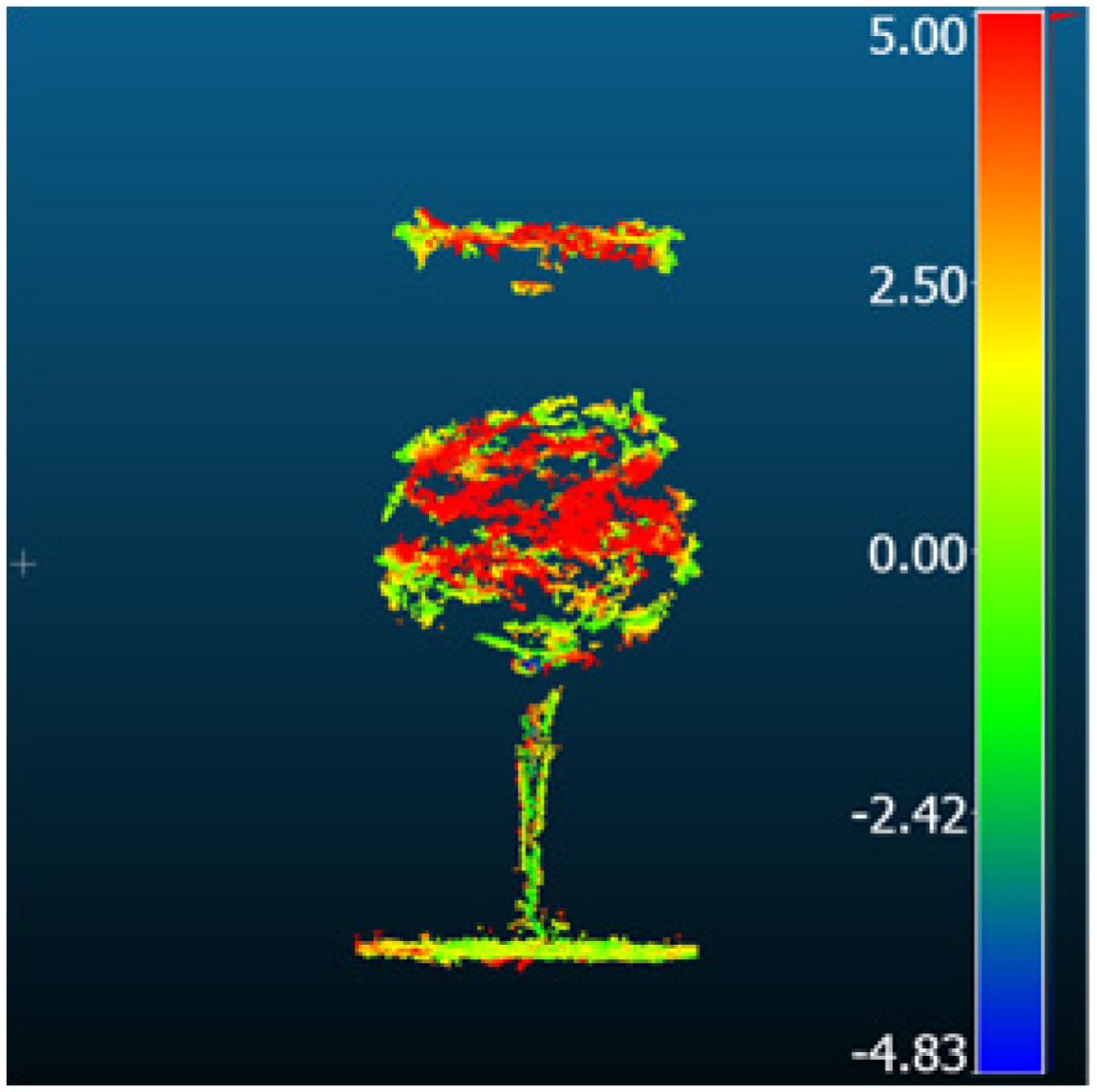 | |
| Method | Gaussian Splatting | Neuralangelo | MVStudio | |
| Metric [mm] | RMSD | 1.54 | 2.29 | 3.14 |
| MAE | 1.22 | 1.72 | 1.69 | |
| STD | 0.93 | 1.51 | 1.43 | |
| Mean_E | 0.44 | 1.19 | 0.93 | |
| Method | ZoeDepth | MiDaS | Depth Anything | ||||||
|---|---|---|---|---|---|---|---|---|---|
| Metric [mm] | RMSD | MAE | STD | RMSD | MAE | STD | RMSD | MAE | STD |
| View_01 | 1.67 | 1.22 | 1.14 | 0.89 | 0.68 | 0.58 | 1.95 | 1.30 | 1.44 |
| View_02 | 1.41 | 1.09 | 0.90 | 1.46 | 1.12 | 0.94 | 1.67 | 1.22 | 1.14 |
| View_03 | 1.19 | 1.01 | 0.86 | 2.08 | 1.56 | 1.38 | 1.28 | 0.99 | 0.82 |
| View_04 | 1.35 | 1.11 | 0.76 | 1.77 | 1.16 | 1.32 | 1.17 | 0.88 | 0.77 |
| Average | 1.41 | 1.11 | 0.92 | 1.55 | 1.13 | 1.06 | 1.52 | 1.10 | 1.04 |
| Standard deviation | 0.20 | 0.09 | 0.16 | 0.51 | 0.36 | 0.37 | 0.36 | 0.20 | 0.31 |
| Method | ZoeDepth | MiDaS | Depth Anything | ||||||
|---|---|---|---|---|---|---|---|---|---|
| Metric [mm] | RMSD | MAE | STD | Metric [mm] | RMSD | MAE | STD | Metric [mm] | RMSD |
| View_01 | 3.95 | 2.80 | 2.79 | View_01 | 3.95 | 2.80 | 2.79 | View_01 | 3.95 |
| View_02 | 3.71 | 2.72 | 2.52 | View_02 | 3.71 | 2.72 | 2.52 | View_02 | 3.71 |
| View_03 | 3.08 | 2.28 | 2.07 | View_03 | 3.08 | 2.28 | 2.07 | View_03 | 3.08 |
| View_04 | 4.22 | 2.62 | 3.31 | View_04 | 4.22 | 2.62 | 3.31 | View_04 | 4.22 |
| Average | 3.74 | 2.61 | 2.67 | Average | 3.74 | 2.61 | 2.67 | Average | 3.74 |
| Standard deviation | 0.49 | 0.23 | 0.52 | Standard deviation | 0.49 | 0.23 | 0.52 | Standard deviation | 0.49 |
| Object | Industrial_A | Sythetic_Metallic | Sythetic_Glass | |
|---|---|---|---|---|
| Best Method | Magic123 | Zero-1-to-3 | Zero-1-to-3 | |
| 3D geometry | 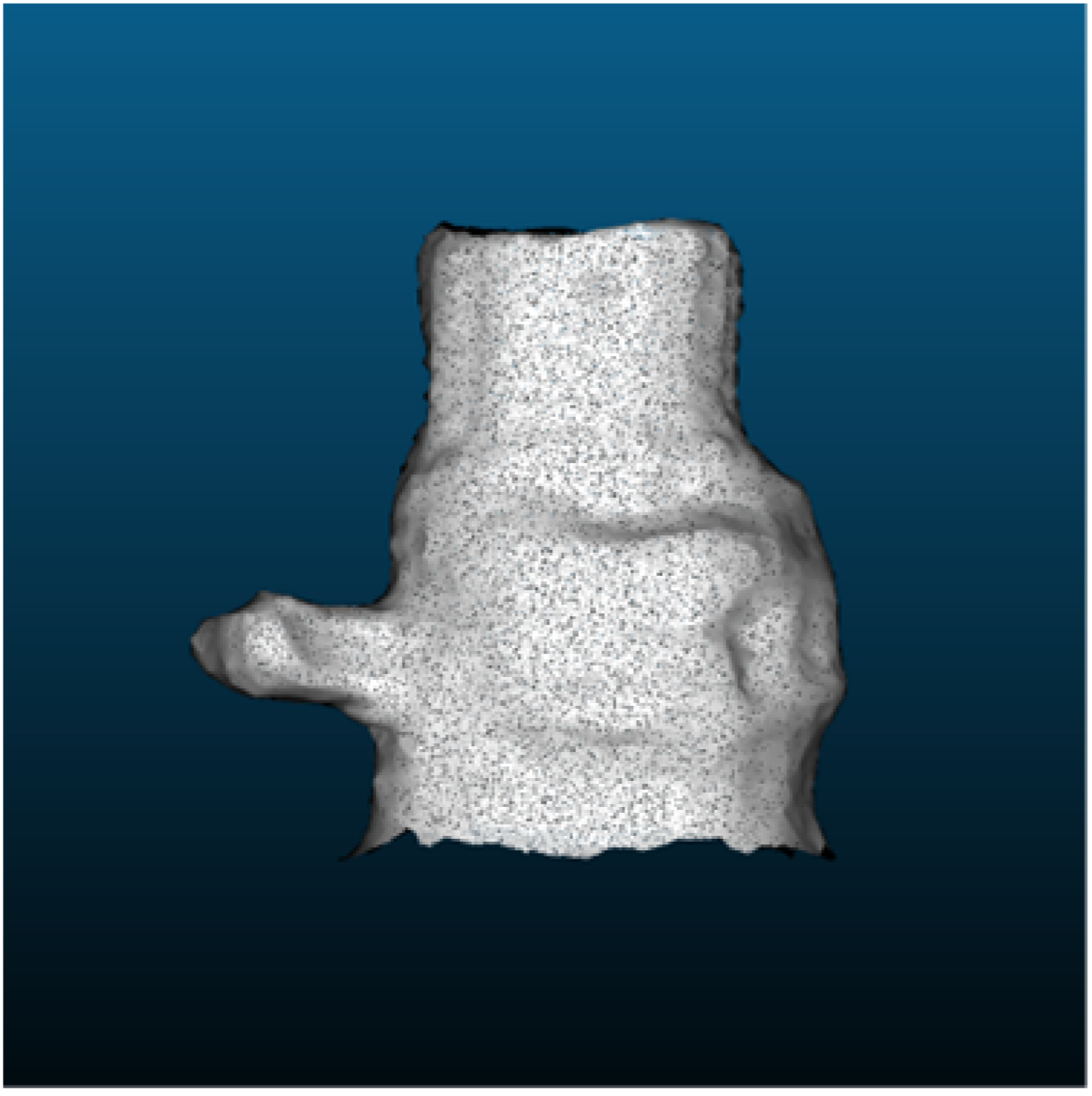 | 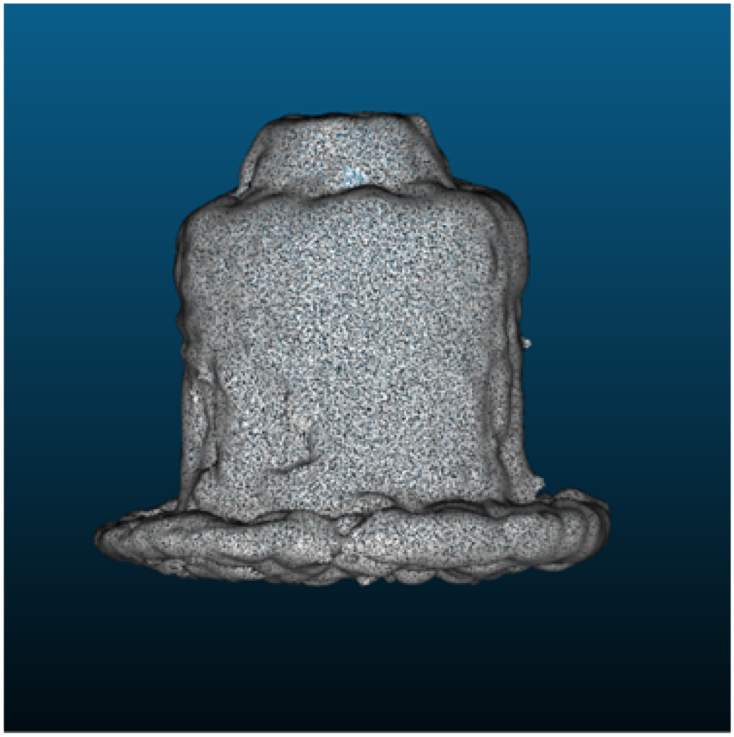 | 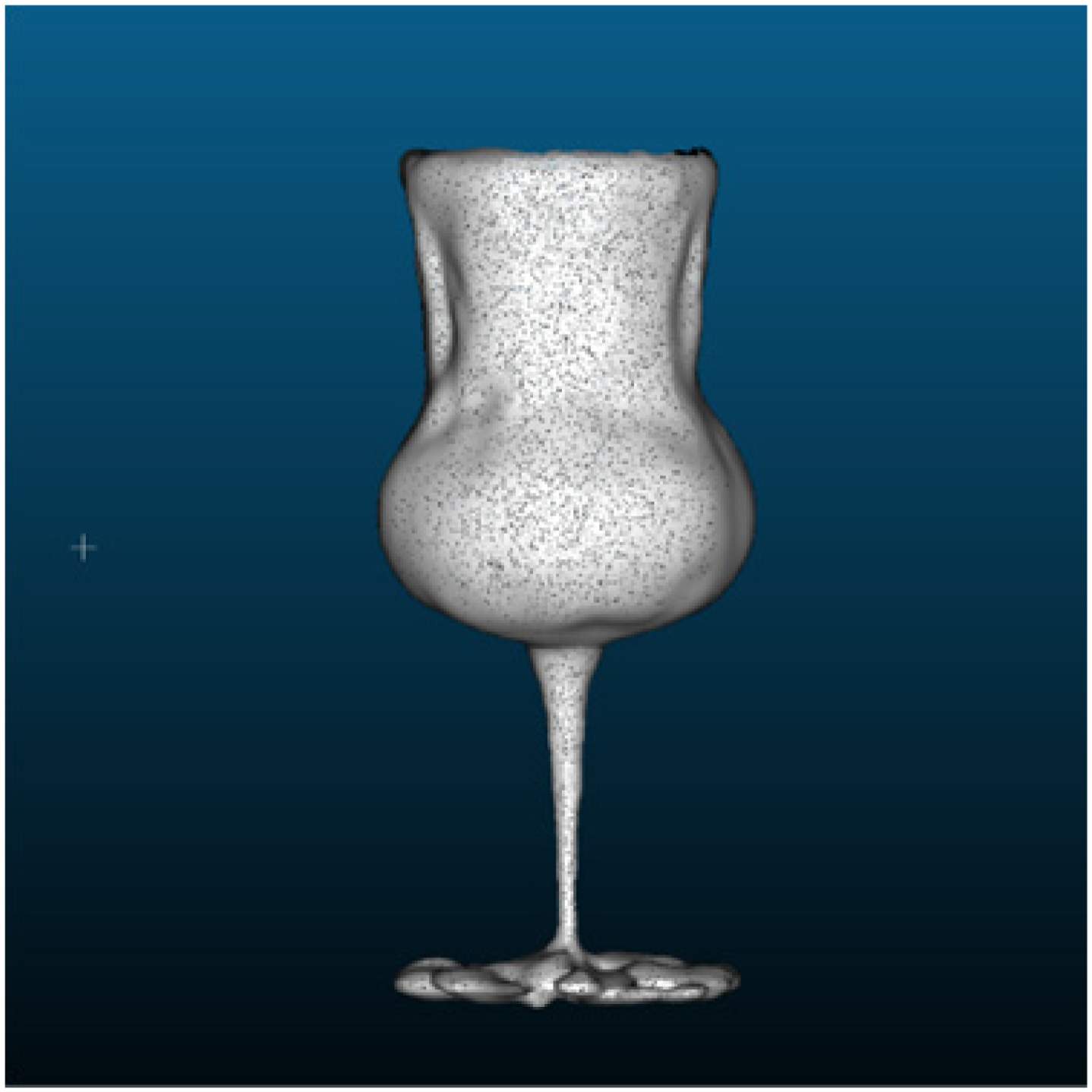 | |
| Comparison result [mm] | 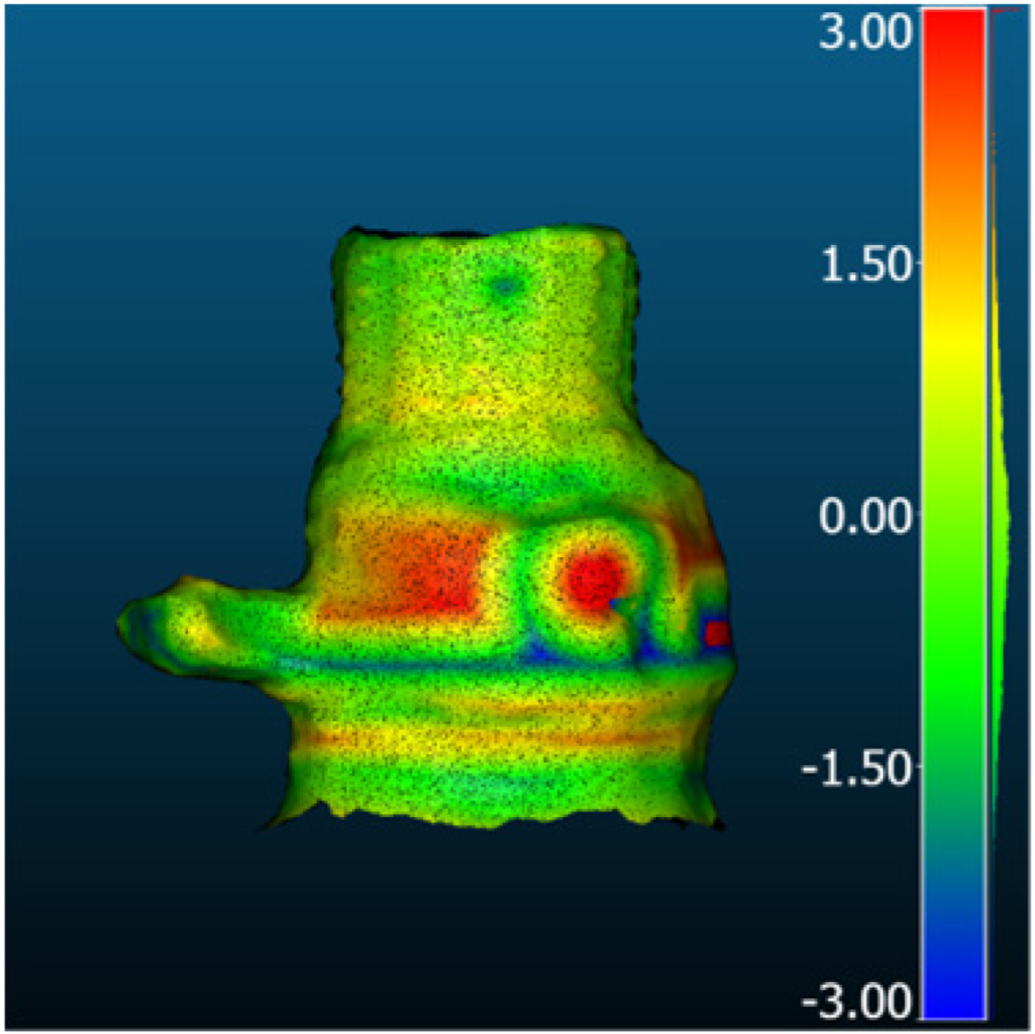 | 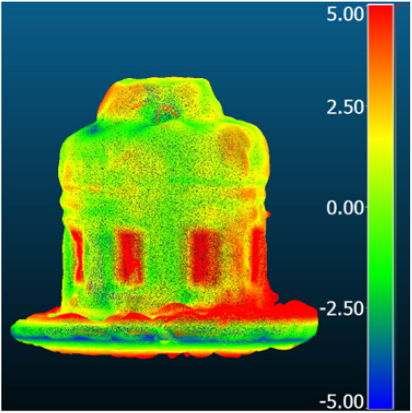 | 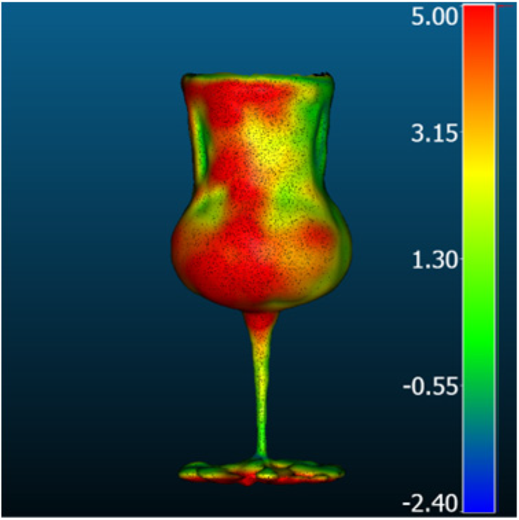 | |
| Metric [mm] | RMSD | 1.12 | 3.08 | 3.32 |
| MAE | 0.88 | 2.46 | 2.76 | |
| STD | 0.68 | 1.84 | 1.85 | |
| Mean_E | −0.04 | 1.26 | 2.39 | |
| Method | Synthetic Metallic | Industrial_A | Synthetic_Glass | |
|---|---|---|---|---|
| NeRF | Instant-NGP |  |  | |
| Mono-Neus | | | | |
| MonoSDF | | | | |
| Mono-Unisurf | | | | |
| Nerfacto(w/depth) | - | | | |
| Nerfacto(w/o depth) | | | | |
| Neuralangelo | | | | |
| NeuS | | | | |
| Neus-Facto | | | | |
| Unisurf | | | | |
| VolSDF | | | | |
| Gaussian Splatting | FSGS | | | |
| GaussianShader | | | | |
| Gaussian Splatting | | | | |
| Scaffold-GS | | | | |
| MVS | DI-MVS | | | |
| ET-MVSNet | | | | |
| GBi-Net | | | | |
| GeoMVSNet | | | | |
| KD-MVS | | | | |
| MVSFormer | | | | |
| MVStudio | | | | |
| TransMVSNet | | | | |
| MDE | Depth Anything | | | |
| MiDaS | | | | |
| ZoeDepth | | | | |
| Generative AI | One-2-3-45 | | | |
| DreamGaussian | | | | |
| Magic123 | | | | |
| Zero-1-to-3 | | | | |
Disclaimer/Publisher’s Note: The statements, opinions and data contained in all publications are solely those of the individual author(s) and contributor(s) and not of MDPI and/or the editor(s). MDPI and/or the editor(s) disclaim responsibility for any injury to people or property resulting from any ideas, methods, instructions or products referred to in the content. |
© 2025 by the authors. Licensee MDPI, Basel, Switzerland. This article is an open access article distributed under the terms and conditions of the Creative Commons Attribution (CC BY) license (https://creativecommons.org/licenses/by/4.0/).
Share and Cite
Yan, Z.; Padkan, N.; Trybała, P.; Farella, E.M.; Remondino, F. Learning-Based 3D Reconstruction Methods for Non-Collaborative Surfaces—A Metrological Evaluation. Metrology 2025, 5, 20. https://doi.org/10.3390/metrology5020020
Yan Z, Padkan N, Trybała P, Farella EM, Remondino F. Learning-Based 3D Reconstruction Methods for Non-Collaborative Surfaces—A Metrological Evaluation. Metrology. 2025; 5(2):20. https://doi.org/10.3390/metrology5020020
Chicago/Turabian StyleYan, Ziyang, Nazanin Padkan, Paweł Trybała, Elisa Mariarosaria Farella, and Fabio Remondino. 2025. "Learning-Based 3D Reconstruction Methods for Non-Collaborative Surfaces—A Metrological Evaluation" Metrology 5, no. 2: 20. https://doi.org/10.3390/metrology5020020
APA StyleYan, Z., Padkan, N., Trybała, P., Farella, E. M., & Remondino, F. (2025). Learning-Based 3D Reconstruction Methods for Non-Collaborative Surfaces—A Metrological Evaluation. Metrology, 5(2), 20. https://doi.org/10.3390/metrology5020020