Accuracy and Repeatability of Rolling Stock Current Distortion Tests for Interference to Signalling

Abstract

The testing of rolling stock for the assessment of disturbance in signalling circuits is considered with a focus on the measurement process and the selection of operating conditions. The definition of interference limits is briefly reviewed, but they are considered an external input. The spectral behavior of acquired signals and the evaluation of repeatability are instead discussed with the help of three different real test cases, considering correspondence between similar operating points and differences as rolling stock operation evolves during a test run. Repeatability evaluated as standard deviation is in the order of 3% to 5% in the harmonic and audio frequency range for the different systems, slightly lower for AC railways; above about 10–15 kHz it increases to 30%. Uncorrelated components (with much lower amplitudes) may show much higher dispersion.

1. Introduction

New and revamped locomotives must undergo a process of certification and one safety-related point is the demonstration by testing of compliance with a range of signaling systems in use in the country in which the locomotive will operate [1,2].

The tests must be exhaustive, covering normal and exceptional operating conditions (OCs): locomotive distortion changes with OCs (traction, cruising, coasting, braking) and the operating point, OP (e.g., the intensity of effort) [3].

The track couples disturbance onto track circuits (TCs) and the return current distribution may vary due to many factors: connections and the arrangement of the return circuit (the number of conductors, transversal bonding, the use of impedance bonds, etc.), rail and track longitudinal impedance, the relative position of the locomotive and traction power station (TPS), soil conditions, and the track-to-earth leakage that modifies the line frequency response (LFR) [4,5,6,7,8,9]. In other words, the transfer function (TF) between the locomotive return current I_l,c through its axles and the track quantities (e.g., rail currents I_r1, I_r2, or rail-to-rail voltage V_r12) is affected by such parameters. This coupling is called “cold path”, to distinguish it from the “hot path” of the TPS current flowing to the locomotive along the catenary (I_l,h). Also, this TF is subject to variability caused by TPS impedance, locomotive–TPS distance, the geometry of conductors, and track parameters [4,5]. I_l,h can be measured more easily than I_l,c, so that, under worst-case assumptions for parameters, configurations, and the number of trains, it can be related to signaling disturbance. This is the approach commonly adopted by administrations to decide the limits to apply to rolling stock (RS).

The assessment of RS distortion against limits is subject to variability, not only in terms of changing RS OCs and the multiple sources onboard, but also because of the overlapping of relevant transients (such as pantograph bounces and inrush phenomena) that require special modeling [10].

The work reviews in Section 2 the main characteristics of signalling circuits and rolling stock, and their interaction, to better understand and discuss test results along with the procedures commented on in Section 3. Several cases of DC and AC rolling stock are analyzed in Section 4, analyzing the variability of measured results, including line impedance and position.

2. Rolling Stock Signaling Interaction

2.1. Rolling Stock

RS consists of a locomotive with coaches or multiple units (known as EMUs) and represents the source of disturbance, caused by traction and auxiliary converters, interfaced by the front-end converter, which for DC systems is a DC/DC buck converter (also known as a chopper) and for AC systems this is a four-quadrant converter (4QC). The return current leaving the axles couples with the affected TC conductively, in differential mode [11,12], whereas the return current in principle flows out the axles symmetrically along the track (two running rails in electric parallel) in both directions. A certain deal of asymmetry exists in the rail–wheel contact resistances, in the coupling between rails of the same and adjacent tracks, and in distributed earthing terms, that transforms the common-mode return current into differential-mode rail current [13]—common transformation values are not larger than 0.1 [11] and this is a first important assumption when fixing safety margins and limits.

Depending on modulation and loading in both cases, lateral components are also present with variable height; whereas for AC vehicles they are at multiples (odd or even) of the fundamental [14], for DC rolling stock there is no clear pattern and various inter-modulation patterns may arise [2].

There is a great variety and variability of distortion patterns [15] and transients (pantograph bounce, wheel slip, overvoltages) [10,16,17], for which the set of tested OCs should be extensive, to comprehend all relevant scenarios plausibly. It is nevertheless important to understand also the variability in supposedly uniform (or identical) OCs. Two such points are discussed in Section 4 based on real measurements.

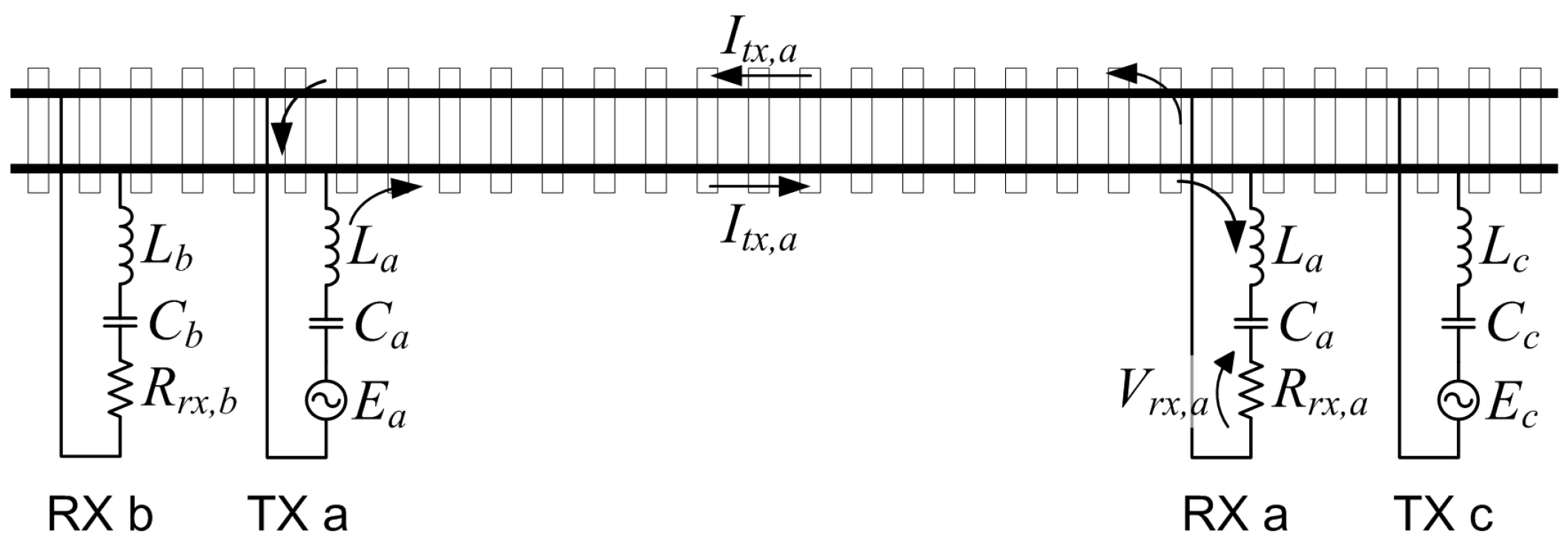
2.2. Signaling Circuits

TCs use a modulated signal sent from a transmitter (TX) to one or two receivers (RX) over the track [11,12]. Track occupation is sensed by measuring the RX signal strength—the occupied status is detected when rails are shunted by the low-resistance axles of the entering RS and the RX signal drops below a threshold (see Figure 1). Operating frequency intervals range from some tens of Hz, for power frequency TCs, up to tens of kHz for audio-frequency (AF) TCs, with rare exceptions.

TX signals are nowadays always coded and modulated (using mostly Frequency Shift Keying, FSK, with a span of some hundreds of Hz, B_RX), making them more robust against disturbance, in particular transients. Limits are, however, specified mainly in amplitude vs. frequency assuming a steady disturbance, although the CLC/TS 50238-2 [18] indicates also a more accurate assessment based on a filter bank approach.

TCs are set up during commissioning to operate with a track voltage intensity that provides the desired flowing current I_tx and signal-to-noise ratio at RX under a range of conditions:

• Poor rolling stock axle resistance (set to 0.25–0.5 Ω values);
• Leaking track causing drainage of RX signal, de facto hiding the shunting axle resistance (normal conductance values can be as low as 1–10 mS/km [19], but commonly applied worst cases can be as high as 0.1–0.5 S/km).

2.3. Line Frequency Response

LFR has been extensively studied [20,21,22], including sensitivity to geometrical and electrical parameters [23]. For what regards this work, it is reminded that:

• Different line sections can show different frequency responses (shifted resonances of different amplitude);
• Anti-resonances are particularly important, as they amplify current components and depend on train position, so they are variable during a test run [24];
• In particular, positioning RS in front of the TPS maximizes current emissions, as line length is minimized, but amplification due to anti-resonances is missed.

2.4. Emission Limit Masks

Limits may be specified for a single frequency (namely a narrow frequency band around the operating frequency of a given TC) or as a whole curve spanning over an extended frequency interval (e.g., covering all possible TC installations of an entire country [25]).

Suitable limits are defined considering all factors discussed in the Introduction that cause TF variability; such limits may be deterministic (mostly) or statistic (so, allowing exceedance if occurring rarely). In the following, limits are considered exact and measurement errors and uncertainty are evaluated forgetting about the underlying margins and assumptions.

3. Testing Methods

The selection of the railway line configuration and rolling stock OCs, which take place first, is followed by the identification of the methods for the measurement, recording, and post-processing of signals. It is worth remembering that at this point the TC is not part of the assessment process, given that its behavior is synthesized in the limit mask with all assumptions, on line configurations, and transfer functions.

3.1. Railway Line and Rolling Stock Operating Conditions

A general attitude by administrations is always using the same line and implicitly comparing the behavior of different rolling stock items over time. In reality, a more solid technical justification would be preferable:

• Either the test line is very simple, so as to reproduce a clear distribution of the return current (such as a single-track straight line with current flowing back in one direction only);
• Or it is a long line reproducing many relevant cases of resonances and anti-resonances, of close proximity to the TPS, etc., with possible issues of mixed traffic.

In general, intense acceleration and braking are applied, but this does not ensure that spectral components at all frequencies would be maximal, only the overall current intensity is maximum; selected OPs could then be added to this aim.

Regarding how measurement results are then processed and used, a common attitude imposed by administrations is using the maximum envelope of measured spectra, in an attempt to provide an additional margin leading to an undisputable worst case. The component’s maxima of course do not occur all at the same time and may belong to different OCs and OPs; in addition, the resulting envelope spectra have a poorer resolution and do not resemble those visible on instruments during tests, compromising physical significance, as a matter of fact. Carefully controlling OCs and OPs ensures that the repeatability of results is not compromised. The use of max-hold envelopes in fact cannot be used as a blanket to hide poor similarity between otherwise identical OCs and OPs.

Repeatability and similarity are in fact an index of the good quality of measurements to be variously processed. Repeatability can be made to correspond to data dispersion, taking repeated measurements under OCs and Ops that are assumed to be the same; that means considering short intervals of adjacent time records or across controlled similar test runs. Similarity instead is a more subjective judgment that is necessary when a purely numeric measure of difference (dispersion) is ineffective, due, e.g., to slight parametric changes in the curves (as caused by different line conditions or driving style) [24,26].

3.2. Measurement and Analysis of Pantograph Current

Accurate measurement and analysis of pantograph current are essential for evaluating the electromagnetic interference (EMI) generated by rolling stock and its potential impact on railway signaling circuits. Two primary analytical methods are employed: Short-Time Fourier Transform (STFT) and Filter-Based Techniques [27,28]. These methods complement each other by offering different perspectives on time–frequency analysis and spectral selectivity, thus contributing to a more comprehensive assessment of interference patterns. This section explores the operational principles, advantages, and limitations of both approaches, emphasizing their complementary roles in achieving accurate and repeatable interference evaluations.

3.2.1. Short-Time Fourier Transform (STFT) Method

The spectrum of disturbance should be evaluated with a frequency resolution δf ≤ B_RX, where BRX represents the bandwidth of the track circuit signal. Using smaller frequency bins allows for rms summation to cover the entire BRX, ensuring detailed spectral analysis, whereas larger bins result in an irreversible loss of necessary resolution. When analyzing data with the Short-Time Fourier Transform (STFT) method, selecting a large δf of tens of Hz (or even up to a hundred) provides a shorter time window T = 1/δf. This approach enhances time resolution, enabling the accurate tracking of the rapidly changing operating points (OPs) of rolling stock. Single FFT spectra obtained for each time window can be composed during post-processing using statistical methods such as max-hold or averaging, thus enabling robust worst-case scenario evaluations.

STFT is particularly effective for observing non-stationary disturbances such as pantograph bounces, inrush currents, and traction harmonics. By segmenting the disturbance signal into short, overlapping windows and applying FFT to each segment, STFT captures the temporal evolution of spectral components, providing a dynamic representation of frequency variations over time. This time–frequency mapping is valuable for correlating spectral changes with the specific operating conditions (OCs) of rolling stock, such as acceleration, cruising, coasting, and braking.

One of the key advantages of STFT is its ability to provide a comprehensive time–frequency representation, allowing for the continuous monitoring of spectral variations corresponding to dynamic OCs. By adjusting the window length, it is possible to balance time and frequency resolution, enabling the detailed tracking of rapidly changing interference patterns. Moreover, the segmented FFT spectra can be combined using various statistical measures, including max-hold, which captures the peak disturbance levels observed across multiple windows, ensuring robust worst-case evaluations.

However, STFT has inherent limitations due to its fixed time–frequency resolution, which is determined by the window length. This fixed resolution imposes a trade-off: shorter windows enhance time resolution but reduce frequency resolution, whereas longer windows improve frequency resolution at the expense of time resolution. This constraint limits the accuracy of narrowband interference isolation, particularly in densely packed spectral environments where precise frequency discrimination is required. Other significant limitations are spectral leakage and smearing, which occur when frequency components change rapidly within a window, resulting in inaccurate spectral representations. Consequently, although STFT provides valuable time–frequency mapping, its fixed resolution and spectral leakage restrict its effectiveness in detailed interference assessments, particularly for high-frequency and narrowband disturbances. Section 4 of this paper utilizes the STFT technique to evaluate the EMI generated by rolling stock under various OCs.

3.2.2. Filter-Based Techniques

Filter-based techniques address some of the limitations of STFT by employing frequency-selective filters that accurately simulate the band-pass characteristics of track circuits. These filters are carefully designed to match the center frequencies, bandwidths, and phase responses of the signaling systems being tested, ensuring a realistic representation of how track circuits respond to both steady-state and transient disturbances. Unlike STFT, filter-based methods maintain a consistent frequency resolution over time, enabling the precise analysis of narrowband interference and dynamic transient events. This makes them particularly suitable for compliance verification against regulatory limits in railway EMI testing.

Three primary types of filters are used in this context: Butterworth, Chebyshev, and Bessel filters. Butterworth filters exhibit a maximally flat frequency response in the passband without ripples, ensuring consistent amplitude characteristics. They are well-suited to broad-spectrum harmonic analysis where minimal amplitude distortion is critical. However, their moderate selectivity and non-linear phase response introduce temporal distortion in transient analysis. Chebyshev filters provide steeper roll-off rates than Butterworth filters, enhancing selectivity for narrowband interference isolation. This is particularly advantageous when adjacent spectral components are densely packed. However, the improved selectivity comes at the cost of ripples in the passband (Type I) or stopband (Type II), which can affect repeatability at high frequencies. Additionally, their non-linear phase characteristics may distort transient signals, limiting their application in time-domain analysis [29].

Bessel filters, on the other hand, are characterized by a maximally linear phase response, preserving the waveform shape of transient signals without introducing phase distortion. This attribute makes them particularly effective for time domain analysis of transient disturbances, such as pantograph bounces and supply transients. However, Bessel filters have a slower roll-off compared to Butterworth and Chebyshev filters, leading to reduced selectivity and higher variability in environments with densely packed spectral components. Despite these limitations, filter-based techniques offer superior frequency selectivity and transient analysis, accurately emulating the operational characteristics of track circuits. They are particularly effective in assessing narrowband disturbances and transient events, providing a more detailed and reliable evaluation of EMI impact on railway signaling systems [29].

3.2.3. Comparative Analysis of STFT and Filter-Based Techniques

While STFT and filter-based techniques offer unique advantages, their limitations necessitate a comparative analysis to determine the most effective approach for different interference scenarios. STFT excels in providing a dynamic time–frequency representation, enabling the continuous monitoring of spectral components as they evolve over time. This capability is particularly useful for correlating frequency variations with changing OCs and OPs. However, its fixed resolution and susceptibility to spectral leakage limit its effectiveness in high-frequency interference analysis. In contrast, filter-based techniques offer superior frequency selectivity and transient analysis due to their consistent frequency resolution and selective filtering capabilities. They provide a more accurate simulation of track circuit behavior, making them indispensable for compliance verification against regulatory limits.

Despite their individual strengths, neither method alone provides a complete solution for interference evaluation. Therefore, a hybrid approach that combines STFT and filter-based techniques is recommended. By leveraging STFT’s dynamic time-frequency mapping with the precise selectivity of filters, this integrated approach maximizes accuracy and repeatability, particularly in transient signal analysis and high-frequency interference evaluation. This hybrid method not only enhances the reliability of interference assessments but also offers a more comprehensive representation of EMI patterns, facilitating better compliance with railway safety standards [18,25].

4. Test Cases

Three different test cases were analyzed, differing in terms of RS and supply system (

Table 1. Summary of test cases and an indication of repeatability among different runs with the same OPs and different OCs expressed as standard deviation vs. mean ratio σ/μ in percentage terms.

System	OCs	N° of Test Runs	σ/μ.	Note
3 kV	ACC	4	3–5%	Correlated components carefully selected
	BRK	4	4–7%
25 kV	ACC	4	2–3%
	BRK	4	2–3%
15 kV	ACC	5	1–3%
	BRK	3	1–3%	Above 15 kHz increase to 30%

). The evaluation of repeatability was achieved by calculating a sample’s standard deviation σ and mean μ among the various runs performed at the same OP for different OCs.

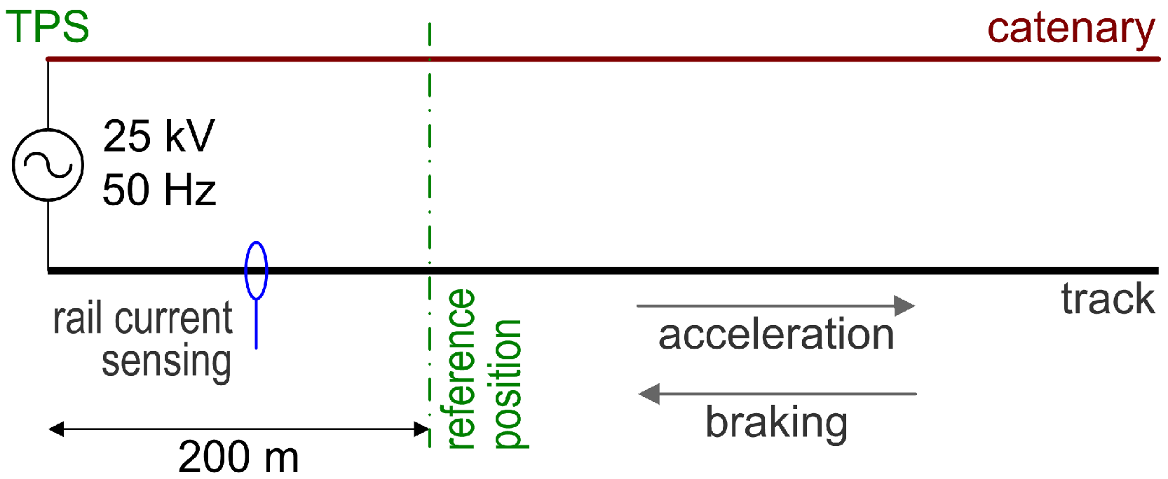
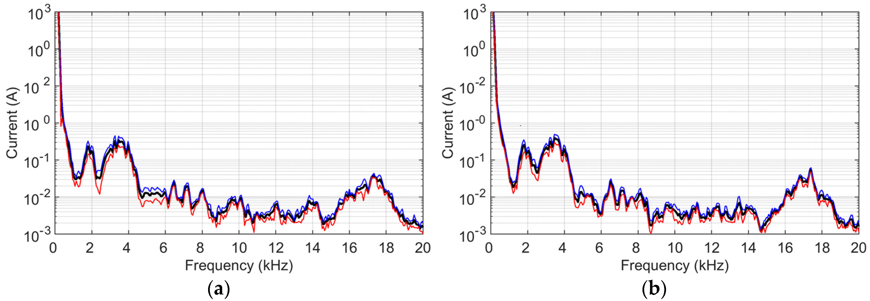
4.1. Single Track 25 kV 50 Hz

A light commuter train with four cars was tested under a 1 × 25 kV 50 Hz supply. The test track was supplied at one end by the Depot TPS and the train was departing from (ACC) or braking to (BRK) a specific reference point, leaving a distance of about 200 m from the TPS according to the test setup shown in Figure 2. The track was arranged by removing cross-bonding connections with the adjacent track, resulting in a single-track configuration. Rail currents were measured in this short section knowing that track leakage was negligible thanks to the short length. The reason for measuring rail current rather than onboard pantograph current was the concomitant test of induction on the wayside cables at the same location and the general difficulty of communication with personnel onboard.

The measurement setup was composed of two LEM Rogowski coils R3030 and RR3030 installed on the two running rails and connected to a HP 35670A 16-bit FFT analyzer in the two available input channels. The Rogowski coils were set in 300 A scale with a sensitivity of 10 mV per A. The analyzer had 800 bins of frequency resolution, thus the measurements were performed by setting the maximum frequency to 25.6 kHz, reaching a resolution of 32 Hz. The measurement chain guaranteed a sensitivity of 1 mA and an uncertainty of ±1% of the measured value up to 20 kHz. The instrumentation used was all calibrated and calibration data were considered for the evaluation of measurement results. Due to the direct measurement in the frequency domain spectrum by the spectrum analyzer, the analysis of measurement variability in the short time over subsequent records could not be performed.

Figure 3 shows the pantograph current spectra measured in acceleration and braking conditions and using the same OPs. Variability was calculated by collecting three test runs, both in ACC and BRK, and the σ/μ ratio ranges between 1% and 3% for all components. It is noted that the frequency resolution being limited by the available instrument’s 800 frequency bins helps to smooth the curves.

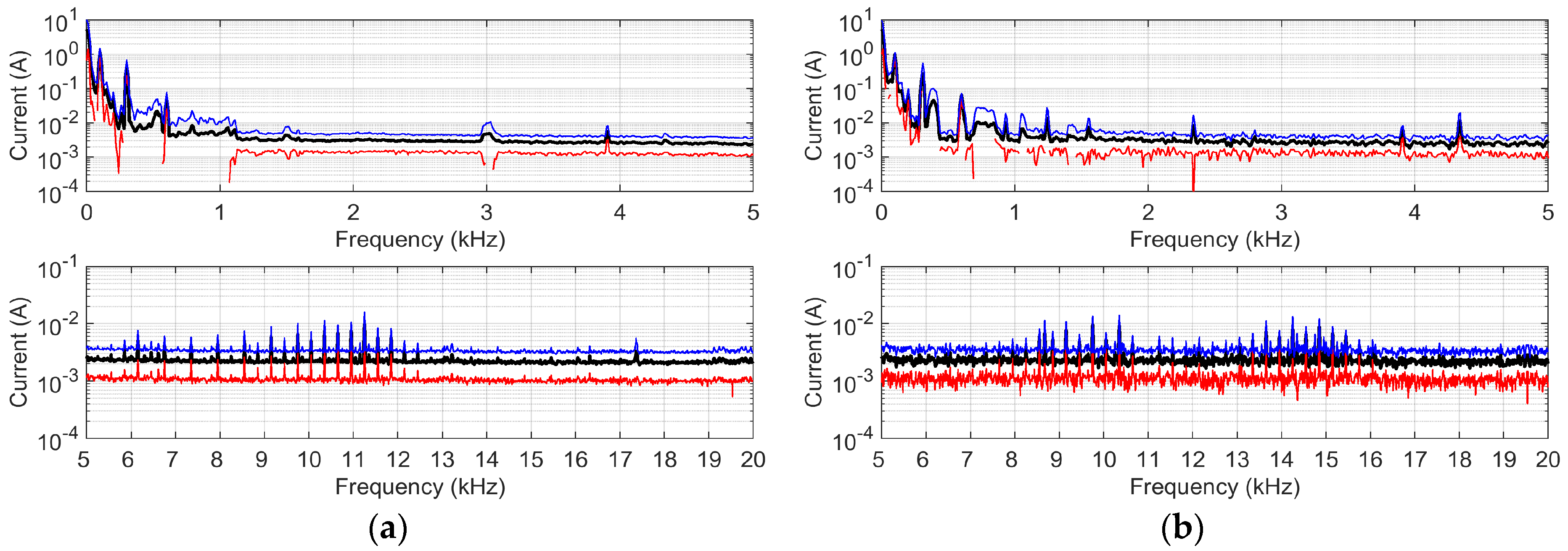
4.2. A 3 kV DC Locomotive on a Real Line

A 3 kV DC 3.5 MW locomotive was tested over about 100 km in Italy, enabling the recording of a wide range of testing conditions (traction, cruising, and braking), but missing an accurate definition of infrastructure conditions met during locomotive runs. Measurements were carried out using a Rogowski LEM R3030 located near the main circuit breaker installed on the busbar inside the vehicle and a Picoscope mod. 4424 (12 bit), sampling at about 200 kHz. The Rogowski probe settings used were a scale set to 30 A or 300 A depending on the oscillation of the vehicle input LC filter that causes some outliers at the lower frequencies. The output sensitivity of the probe was set to 10 mV/A and the picoscope input range to ±2 V. Considerations regarding the measurement uncertainty of the measurement chain are reported in [30]. The instrumentation used was all calibrated and the calibration data were used during the measurements.

Figure 4 shows the pantograph current spectra measured in acceleration and braking conditions and using the same OPs; DC traction current harmonics are more variable compared to AC, as no fundamental is available, except for the known TPS harmonics. The analysis was performed then only for those components clearly correlated with RS emissions. Variability over the four runs was 3–5%, whereas values > 30% may characterize uncorrelated components. A correlation analysis of I_p and V_p (not recorded), would have helped to isolate RS emissions using methodology already shown in the existing research [3,29]. Pantograph voltage is, however, rarely measured, if not strictly necessary, due to safety issues associated with connecting to a high-voltage circuit. During recordings many out-of-scale measurements were observed due to onboard filter oscillations [16], making captured waveforms asymmetrical and causing spectrum leakage. Tapering windows may be used with moderate spectral leakage, but not when the low-frequency oscillation is much larger than the components subject to analysis, and such records must be discarded.

4.3. 15 kV AC Locomotive on Real Line

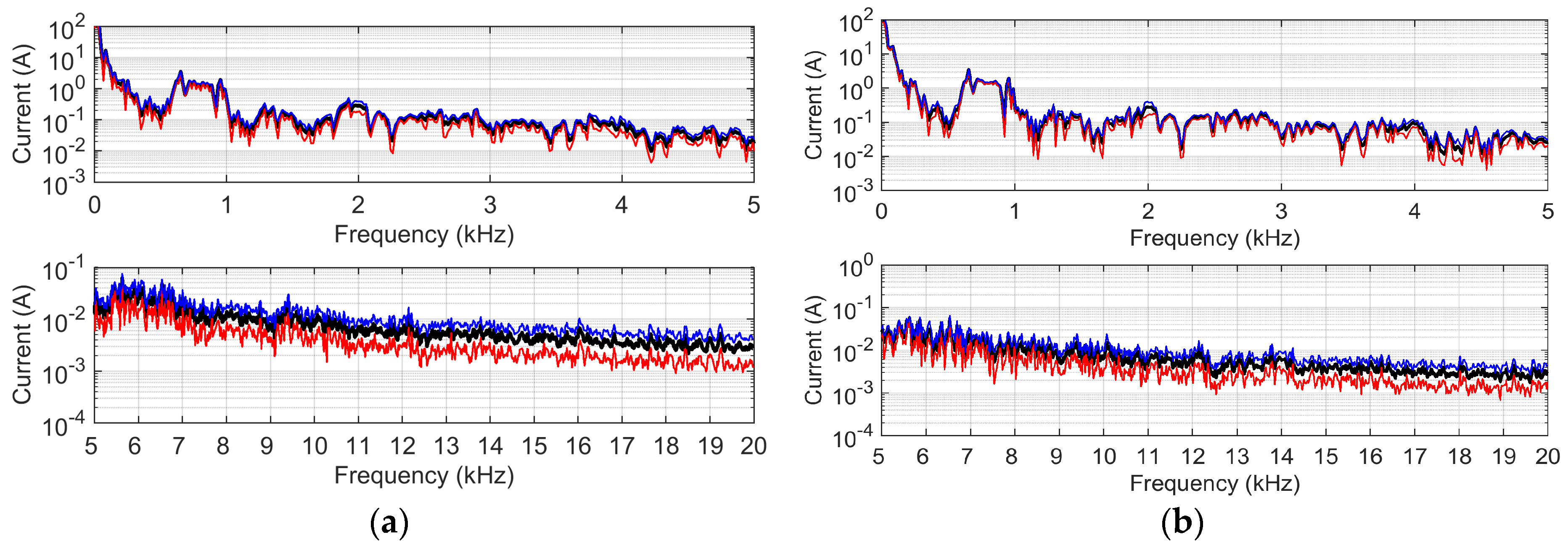
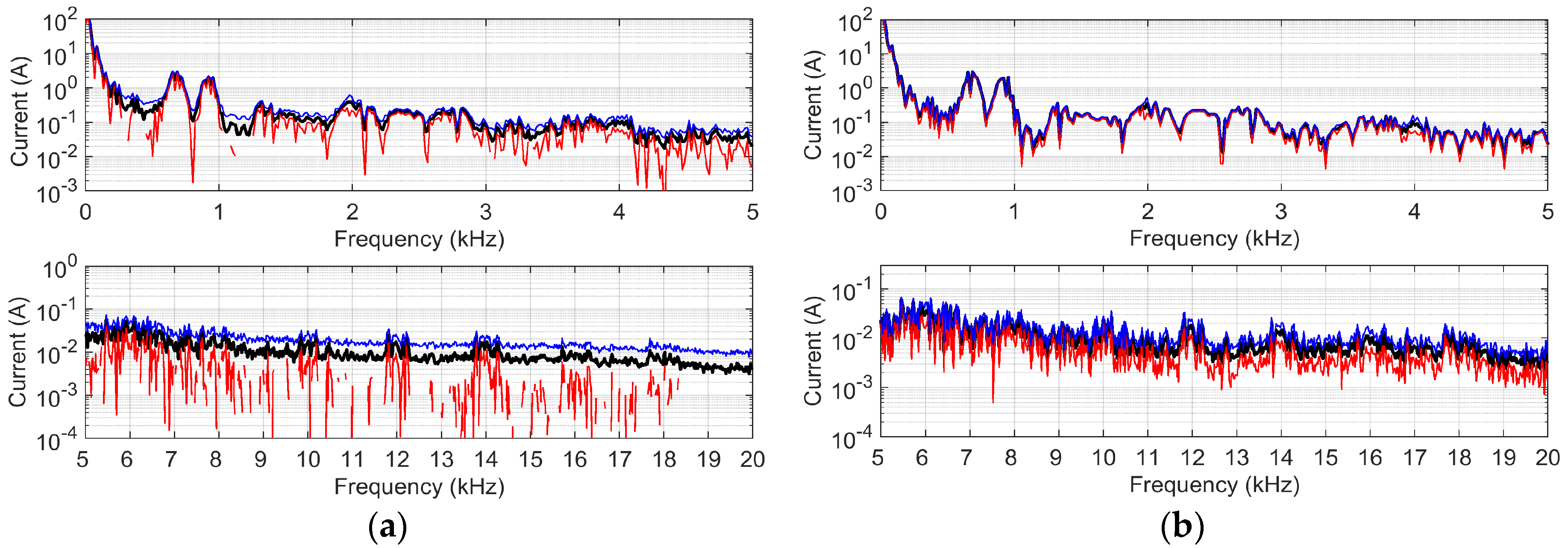
A 15 kV 16.7 Hz Swiss passenger train equipped with an Re460 locomotive was tested using a LEM Rogowski coil mod. R3030 (20 kHz bandwidth) and a 16-bit Dewetron data acquisition system sampling at 50 kHz [28]. The measurement chain guaranteed a sensitivity of 10 mA and an uncertainty of ±1.2% of the measured value up to 20 kHz. The instrumentation used was all calibrated and the calibration data were considered in the measurement results. The large amount of usable data in this case made it possible to evaluate repeatability in various OCs and OPs at four different locations. The differences in terms of variability of measurement performed using same OCs in different locations along the line and using different OCs in the same location are shown both for acceleration (Figure 5) and braking (Figure 6) conditions.

The standard deviation is calculated for all frequency samples although it should be considered only for the RS emission components. The FFT resolution is 16.7 Hz, focusing on the expected harmonics of the 4QC converter. Repeatability is some%, but data abundance allows these considerations:

• Amplitude distribution is asymmetric, more compact at the highest levels of emission with a long tail towards very small values, so that dispersion does not transfer straightforwardly to an estimate of uncertainty;
• Repeatability in ACC and BRK is in the order of 3% for RS emission components with the minimum influence of the infrastructure for most of them (so, for the same OP and the same or different locations);
• LFR resonances have a significant effect at high frequencies, so that above 15 kHz repeatability worsens by an order of magnitude (about 30%); this is also due to some movement between adjacent frequency bins due to a slight fundamental instability.

5. Conclusions

This study provides a comprehensive evaluation of the accuracy and repeatability of rolling stock distortion tests for assessing electromagnetic interference (EMI) with railway signaling circuits. A high repeatability (3–5%) was observed in the harmonic and audio frequency ranges, while variability increased significantly above 15 kHz and when comparing measurements performed with the same operating conditions (OCs) and operating points (OPs) at different locations along the line (up to 30%), due to line frequency response (LFR) resonances and infrastructure characteristics. These findings highlight the importance of a consistent selection of operating conditions (OCs) and operating points (OPs) to improve measurement quality and reduce uncertainty due to the variability of system conditions in terms of measurement results. The analysis of measurements performed at the same OCs and OPs at different locations along the line, although not representative of the worst cases or of the whole variability of the current emissions that may appear in real cases due to the interaction of the vehicle and infrastructure, highlight the need to use a limited and accurately evaluated stretch of line when the purpose is achieving the metrological accuracy of the measurements. It is, however, worth noting that safety limits to ensure safety in all operating and system conditions have a safety margin with respect to the real susceptibility of the track circuit receiver that covers all variabilities in terms of imbalance and resonances.

The comparative analysis demonstrates that Short-Time Fourier Transform (STFT) is effective for dynamic time–frequency representation, making it suitable for tracking transient events and spectral variations over time. However, its fixed resolution and susceptibility to spectral leakage limit its effectiveness for detailed interference analysis, particularly at high frequencies. In contrast, Filter-Based Techniques provide superior frequency selectivity and transient analysis by accurately simulating the band-pass characteristics of track circuits. They offer consistent frequency resolution over time, enabling precise analysis of narrowband interference and dynamic transient events. This study suggests that integrating Filter-Based Techniques into interference evaluation methodologies can significantly enhance accuracy and repeatability. Although filter-based methods provide more detailed spectral selectivity, further research is needed to optimize their design parameters for different signaling environments. Additionally, the lack of direct comparative studies between filter-based and STFT methods highlights the need for future research to provide a systematic comparison of their performance under identical operating conditions. This would establish a clearer understanding of their relative advantages and limitations.

Future research should focus on the systematic integration of Filter-Based Techniques into existing interference evaluation frameworks. This includes performing direct comparative studies between filter-based and STFT methods under identical OCs and OPs to quantify their relative performance and determine the optimal scenarios for each technique. Such comparisons would establish a more standardized approach to EMI evaluation. Moreover, the development of hybrid analysis models that combine the dynamic time–frequency mapping of STFT with the precise selectivity of filter-based methods is recommended. These hybrid models would leverage the strengths of both techniques, enhancing transient signal analysis and high-frequency interference evaluation.

Additionally, filter-based techniques should be expanded to include more detailed spectral analysis of transient signals, particularly in hybrid cases where rapid spectral changes occur. The integration of these methods would provide a more comprehensive representation of EMI patterns and improve compliance with railway safety standards.

By advancing these methodologies, future studies will contribute to the development of more robust and accurate electromagnetic compatibility testing frameworks for railway systems. This approach not only enhances interference evaluation accuracy but also ensures safer and more reliable railway signaling systems.

References

- Havryliuk, V.; Serdyuk, T. Distribution of harmonics of return traction current on feeder zone and evaluation of its influence on the work of rail circuits. In Proceedings of the 18th International Wroclaw Symposium and Exhibition on Electromagnetic Compatibility, Wroclaw, Poland, 28–30 June 2006; pp. 467–470. [Google Scholar]
- Steczek, M.; Szelag, A.; Chatterjee, D. Analysis of disturbing effect of 3 kV DC supplied traction vehicles equipped with two-level and three-level VSI on railway signalling track circuits. Bull. Pol. Acad. Sci. Tech. Sci. 2017, 65, 663–674. [Google Scholar] [CrossRef]
- Mariscotti, A. Non-Intrusive Load Monitoring Applied to AC Railways. Energies 2022, 15, 4141. [Google Scholar] [CrossRef]
- Bongiorno, J.; Mariscotti, A. Variability of pantograph impedance curves in DC traction systems and comparison with experimental results. Przegląd Elektrotech. 2014, 90, 178–183. [Google Scholar]
- Ferrari, P.; Mariscotti, A.; Pozzobon, P. Reference curves of the pantograph impedance in DC railway systems. In Proceedings of the IEEE International Conference on Circuits and Systems, Geneve, Switzerland, 28–31 May 2000. [Google Scholar]
- Dolara, A.; Gualdoni, M.; Leva, S. EMC disturbances on track circuits in the 2 × 25 kV high speed AC railways systems. In Proceedings of the IEEE PES Trondheim PowerTech 2011, Trondheim, Norway, 19–23 June 2011. [Google Scholar]
- Huang, W.; He, Z.; Hu, H.; Wang, Q. Study on Distribution Coefficient of Traction Return Current in High-Speed Railway. Energy Power Eng. 2013, 5, 1253–1258. [Google Scholar] [CrossRef]
- Nair, R.K.; Saini, D.K.; Jayaraju, M. Dynamism of Parasite Capacitance of AC Electric Traction Line Inside the Railway Tunnels. IETE J. Res. 2022, 68, 1358–1365. [Google Scholar] [CrossRef]
- Mariscotti, A. Impact of Rail Impedance Intrinsic Variability on Railway System Operation, EMC and Safety. Int. J. Electr. Comput. Eng. 2021, 11, 17–26. [Google Scholar] [CrossRef]
- Bongiorno, J. Induced touch voltage in wayside cables of AC railways caused by traction supply transients. Electr. Eng. 2023, 105, 13–24. [Google Scholar] [CrossRef]
- Mariscotti, A.; Ruscelli, M.; Vanti, M. Modeling of Audiofrequency Track Circuits for validation, tuning and conducted interference prediction. IEEE Trans. Intell. Transp. Syst. 2010, 11, 52–60. [Google Scholar] [CrossRef]
- Zhao, L.; Li, M. Probability Distribution Modeling of the Interference of the Traction Current in Track Circuits. J. Theor. Appl. Inf. Technol. 2012, 46, 125–131. [Google Scholar]
- Razghonov, S.; Kuznetsov, V.; Zvonarova, O.; Chernikov, D. Track circuits adjusting calculation method under current influence traction interference and electromagnetic compatibility. Mater. Sci. Eng. 2020, 985, 012017. [Google Scholar] [CrossRef]
- Mariscotti, A. Results on the Power Quality of French and Italian 2 × 25 kV 50 Hz railways. In Proceedings of the I2MTC 2012, Graz, Austria, 13–16 May 2012. [Google Scholar]
- Salles, R.S.; De Oliveira, R.A.; Rönnberg, S.K.; Mariscotti, A. Analytics of Waveform Distortion Variations in Railway Pantograph Measurements by Deep Learning. IEEE Trans. Instrum. Meas. 2022, 71, 2516211. [Google Scholar] [CrossRef]
- Mariscotti, A.; Giordano, D. Experimental characterization of pantograph arcs and transient conducted phenomena in DC railways. Acta Imeko 2020, 9, 10–17. [Google Scholar] [CrossRef]
- Nicolae, P.M.; Nicolae, M.S.; Nicolae, I.D.; Netoiu, A. Overvoltages Induced in the Supplying Line by an Electric Railway Vehicle. In Proceedings of the IEEE International Joint EMC/SI/PI and EMC Europe Symposium, Raleigh, NC, USA, 26 July–13 August 2021; pp. 653–658. [Google Scholar]
- CLC/TS 50238-2; Railway Applications—Compatibility Between Rolling Stock and Train Detection Systems—Part 2: Compatibility with Track Circuits. CENELEC Standard: Brussels, Belgium, 2015.
- Mariscotti, A.; Pozzobon, P. Experimental results on low rail-to-rail conductance values. IEEE Trans. Veh. Technol. 2005, 54, 1219–1222. [Google Scholar] [CrossRef]
- Dolara, A.; Gualdoni, M.; Leva, S. Impact of High-Voltage Primary Supply Lines in the 2 × 25 kV—50 Hz Railway System on the Equivalent Impedance at Pantograph Terminals. IEEE Trans. Power Deliv. 2012, 27, 164–175. [Google Scholar] [CrossRef]
- Ceraolo, M. Modeling and Simulation of AC Railway Electric Supply Lines Including Ground Return. IEEE Trans. Transp. Electrif. 2017, 4, 202–210. [Google Scholar] [CrossRef]
- Serdiuk, T.; Serdiuk, K. Mathematic modeling of distribution of traction current harmonics. In Proceedings of the Joint IEEE International Symposium on Electromagnetic Compatibility Signal and Power Integrity, and EMC Europe, EMC/SI/PI/EMC Europe, Raleigh, NC, USA, 26 July 2021; pp. 659–662. [Google Scholar]
- Garg, R.; Mahajan, P.; Kumar, P. Sensitivity Analysis of Characteristic Parameters of Railway Electric Traction System. Int. J. Electron. Electr. Eng. 2014, 2, 8–14. [Google Scholar] [CrossRef]
- Bongiorno, J.; Mariscotti, A. Experimental validation of the electric network model of the Italian 2 × 25 kV 50 Hz railway. In Proceedings of the 20th IMEKO TC4 Symposium on Measurements of Electrical Quantities, Benevento, Italy, 15–17 September 2014; pp. 964–970. [Google Scholar]
- CLC/TR 50507; Railway Applications—Interference Limits of Existing Track Circuits Used on European Railways. CENELEC Standard: Brussels, Belgium, 2007.
- Bongiorno, J.; Mariscotti, A. Robust estimates for validation performance indexes of electric network models. Int. Rev. Electr. Eng. 2015, 10, 607–615. [Google Scholar] [CrossRef]
- Mariscotti, A. Variability and uncertainty of Track Circuit band-pass modeling for interference evaluation. Acta Imeko 2013, 2, 32–39. [Google Scholar] [CrossRef]
- Bhagat, S.; Mariscotti, A. Interference with Signaling Track Circuits Caused by Rolling Stock: Uncertainty and Variability on a Test Case. Electronics 2024, 13, 2875. [Google Scholar] [CrossRef]
- Bongiorno, J.; Mariscotti, A. Recent results on the power quality of Italian 2 × 25 kV 50 Hz railways. In Proceedings of the 20th IMEKO TC4 Symposium on Measurements of Electrical Quantities, Benevento, Italy, 15–17 September 2014; pp. 953–957. [Google Scholar]
- Mariscotti, A. Data sets of measured pantograph voltage and current of European AC railways. Data Brief 2020, 30, 105477. [Google Scholar] [CrossRef] [PubMed]