Measurement and Simulation of Demagnetization in a Prototype Halbach Array Quadrupole

Abstract

We present the design, construction, measurement, and troubleshooting of a prototype hybrid Halbach quadrupole magnet. This magnet was significantly under-strength due to local demagnetization in the permanent magnet material. We discuss how this effect was uncovered, how it was verified by performing Hall probe measurements of the individual magnet blocks, and how the effect was reconstructed in simulations.

1. Introduction

Permanent magnets can, for some particle accelerator-related uses, have significant advantages over more traditional electromagnets. For many uses, the key advantage is that the power consumption of an electromagnet is avoided, and by extension, the needs and costs of power delivery infrastructure and active cooling are also avoided. This advantage becomes particularly prevalent in cases where the magnet is required to be located entirely within a vacuum chamber, where supply of power and water to an electromagnet is complicated as is the removal of the thermal energy released by resistive electromagnetic coils. Additionally, by arranging permanent magnet blocks in a Halbach configuration [1], it is possible to achieve extremely strong magnetic fields or magnetic field gradients in the case of a quadrupole arrangement. Gradients of up to 500 T/m have been demonstrated [2], albeit typically only over a small magnet aperture and with lower gradient homogeneity than more traditional magnet designs.

We focus here on the case of quadrupole magnets that form a capture channel for electrons emitted from laser-plasma wakefield accelerators [3], a technique for rapidly accelerating electrons, which has garnered wide attention in recent years. In this case, the high source divergence and potential large energy spread demands that magnets must be very strong (gradients of 300–500 T/m) and are typically located in-vacuum very close to the electron source [4,5,6]. It is, therefore, apparent that this situation is one where the advantages of permanent magnets listed above are prevalent. The Halbach array quadrupole is a well-suited design to this task, capable of producing strong gradients whilst being relatively easy to engineer for vacuum compatibility. Halbach array magnets (and magnets incorporating aspects of the Halbach design) have been used for this and similar purposes before [7,8,9,10,11], including with some novel schemes for allowing the field strength to be tuned over a wide range [12,13,14].

The Accelerator Science & Technology Centre (ASTeC) at STFC Daresbury Laboratory (UK) has collaborated with the Extreme Photonics Applications Centre (EPAC) [15] at STFC Rutherford Appleton Laboratory (UK) to design and build a prototype hybrid Halbach quadrupole for capturing electrons accelerated by a petawatt-class laser pulse in a plasma [16,17,18]. The EPAC facility intends to produce 1 PW laser pulses at a repetition rate of 10 Hz, which will be focused through a gas cell, generating a plasma and performing laser wakefield acceleration of electrons to energies up to 5 GeV. Early experiments expect to generate broadband beams in the range of 1 GeV before the energy spread is reduced and central energy increased as the technique is refined. The quadrupole is designed to operate in an array of 4, 8, or 10 identical magnets that will perform the initial capture of the electron beam, with the first quadrupole positioned just 50 mm from the exit of the plasma cell. The array is designed for the capture of a 1 GeV beam but is adaptable to other energies by changing the spacing between the magnets.

2. Quadrupole Magnet Design

The target strength of the quadrupoles is 500 T/m as determined by beam physics simulations. The magnetic length is 50 mm. The necessary clear aperture is 8 mm diameter to allow for unobstructed passage of both the broadband electron beam and the laser pulse, which passes through the aperture of the first quadrupole before being extracted by a plasma mirror on a Kapton tape drive.

It was determined that the optimal configuration of the quadrupole would be a hybrid Halbach type [19], although pure permanent magnet Halbach types were considered. The drawback of the pure permanent magnet array was that the achievable gradient homogeneity was found to be too poor in simulations once realistic errors in block size and strength were taken into account and there was no simple method for shimming the field strength without changing aperture, which made the overall magnet dimensions far too large for the EPAC chamber.

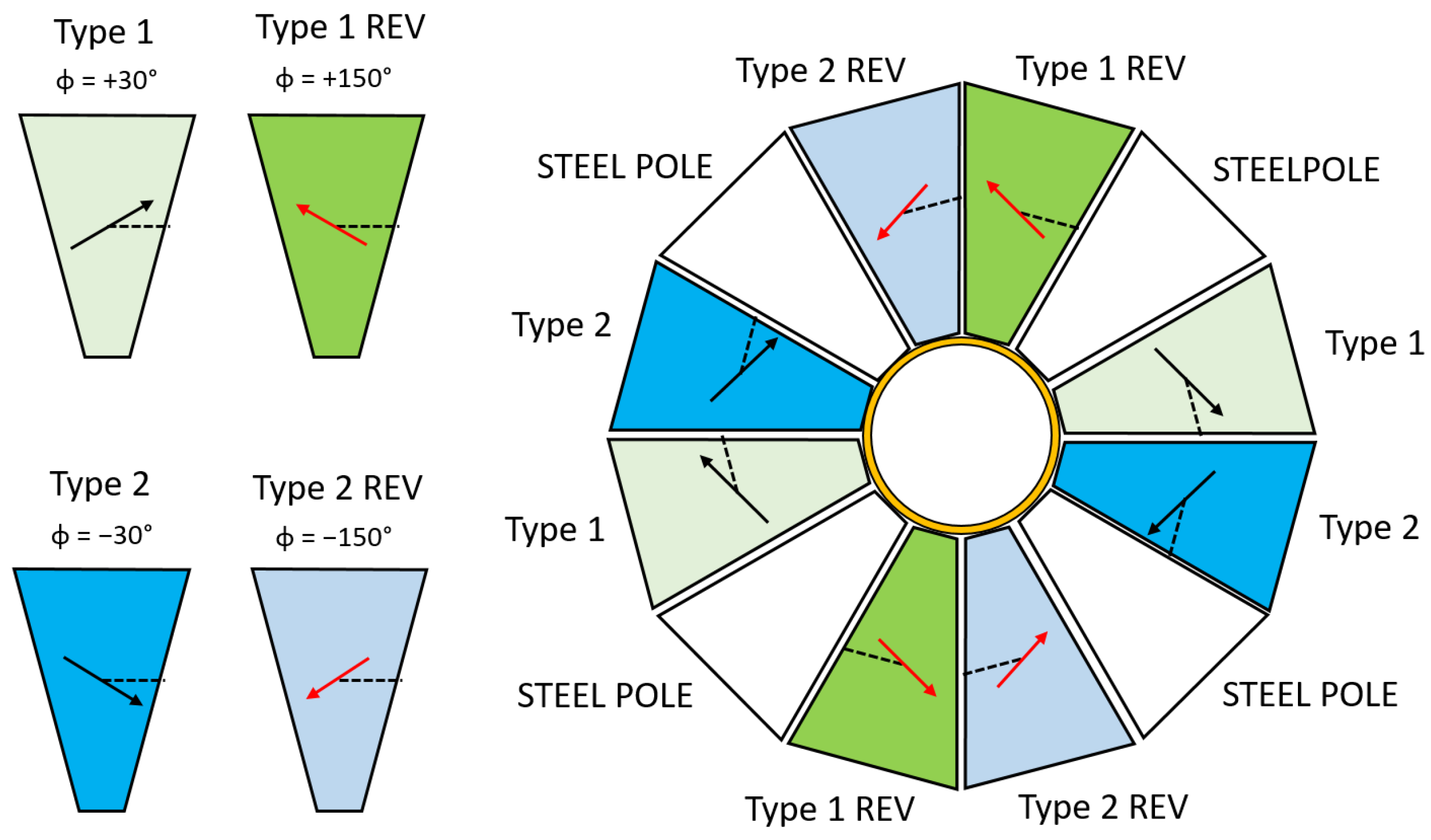
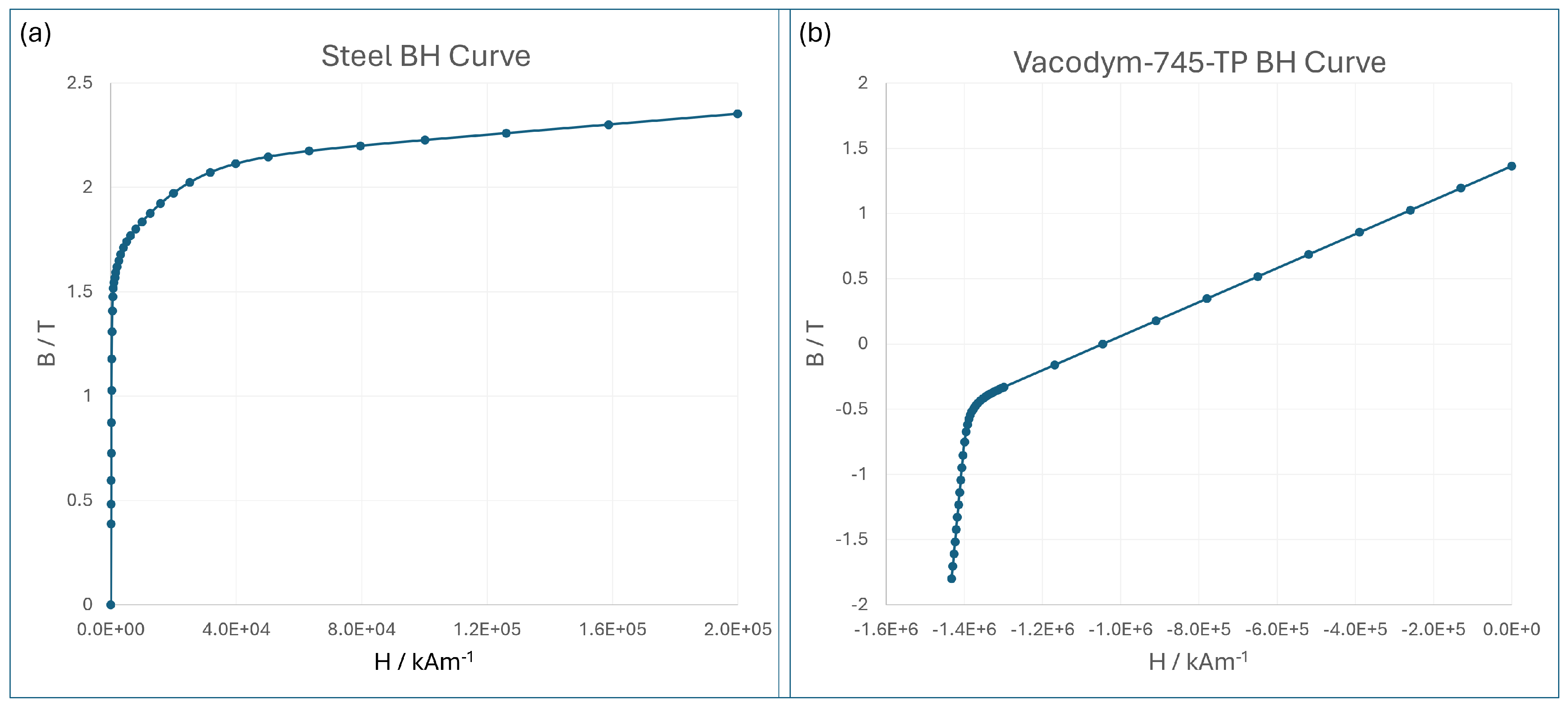
The hybrid Halbach array is composed of a circular series of 12 wedges. The permanent magnet material comprises eight of these wedges and provides the entirety of the flux. The magnet wedges are Neodymium–Iron–Boron (NdFeB). The specific material is VACODYM-745-TP, which has a minimum remanent flux density $B_r$ of 1.37 Tesla and a coercivity $H_c$ of −1035 kA/m. This material is a proprietary grade of NdFeB produced by Vacuumschmelze (Hanau, Germany). This material was chosen because of its high remanent flux density. At the design stage, the demagnetization effects, which would have been mitigated by the use of a higher coercivity material, were not predicted. The remaining four wedges act as magnet poles made from high-permeability steel. In the initial design, these were Cobalt–Iron due to its high saturation flux density. However, in the final design and the prototype discussed here, they were manufactured from AISI grade 1006 steel for cost-saving purposes. The simulations, design, and assembly procedure of this quadrupole are presented in detail in [20] and so are not presented in detail here. 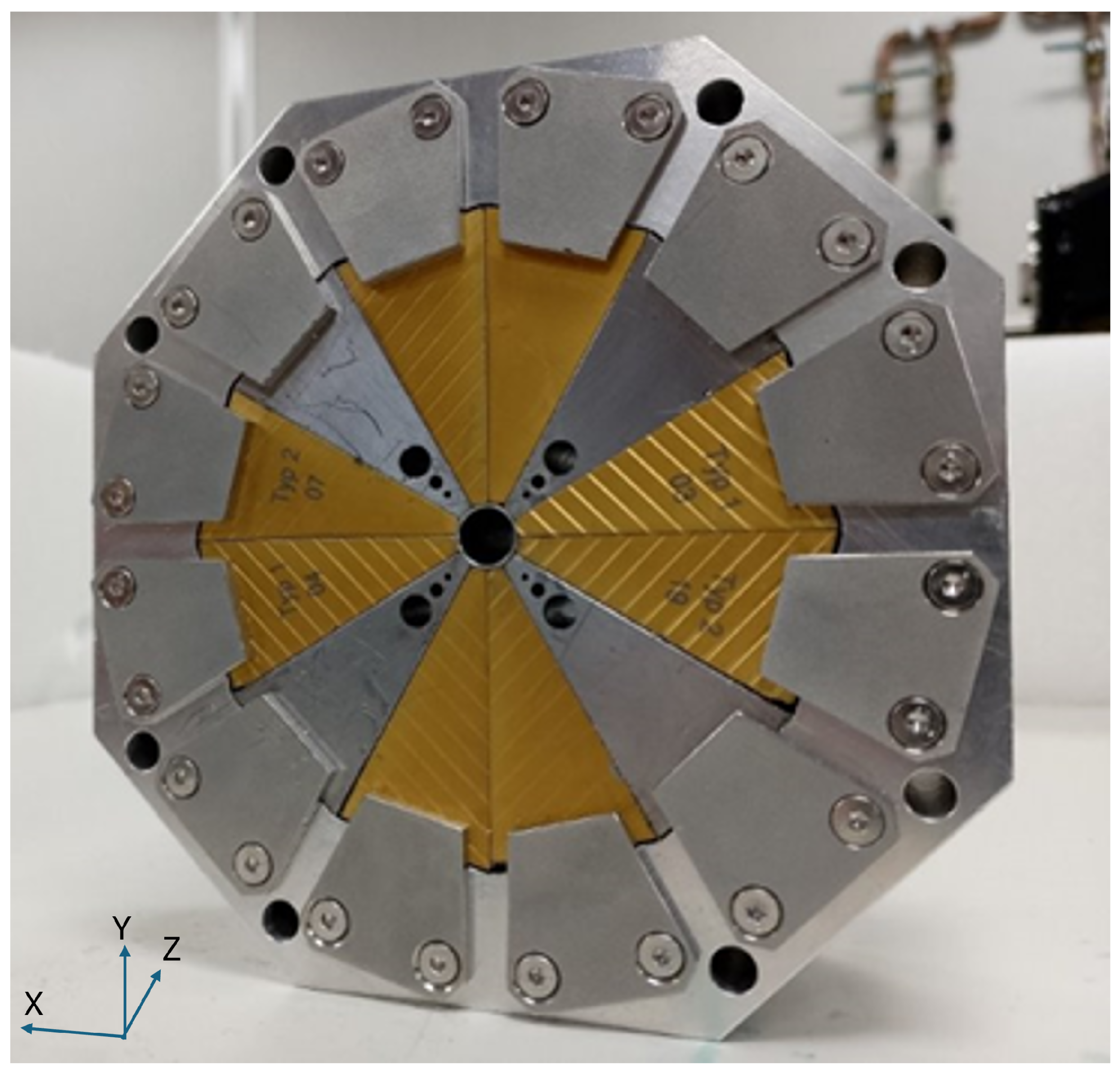Figure 1 shows the magnetization vectors of the magnet blocks, and the final constructed magnet is shown in Figure 2.

The magnetic modelling of the quadrupole was performed using SIMULIA Opera™ Finite Element Analysis (FEA) software (version 2022 for initial design, version 2023 for work presented here) [21], employing the built-in magnetostatic solver. Non-linear modelling was employed where material BH curves for all materials were used across several model iterations, instead of simple relative magnetic permeabilities, to account for realistic non-linear behaviour in the materials as a function of magnetic flux density. This is discussed in more detail in Section 4. It is of relevant note to the following sections that this solver does not include the modelling of permanent changes to material magnetization, which requires applying a separate solver to the model.

The magnet has a tuneable gradient via the insertion or removal of steel rods (tuning pins) through varying-sized holes in each of the steel poles. The details of this are discussed in [20]. The gradient with no tuning pins inserted was predicted to be 485 T/m, which could be increased to 514 T/m with all 12 tuning rods in place. The magnet length is 50 mm, and the magnetic aperture is 9 mm (of which 8 mm is clear aperture and the rest is an aluminium structural tube).

Measurements determined that these magnets produced a gradient of 340 T/m across a 9 mm aperture instead of the predicted gradient of 485 T/m for the tuning configuration at which the measurements were performed. We present in the sections below the measurements and simulations undertaken in the investigation of this discrepancy, revealing and quantifying significant demagnetization in the magnet blocks.

3. Initial Measurements

After assembly at Daresbury Laboratory, the quadrupole was measured using a Senis (Zug, Switzerland) 3MH3 Fluxmeter with a type H 3-axis Hall probe mounted on a precision 3-axis motion system. The system utilizes stepper motors and absolute encoders to achieve single μm precision in the transverse and vertical planes and 10 μm precision in the longitudinal plane. A granite bench provided vibration isolation to the probe, although the magnet itself was mounted on a separate table next to the bench and did not benefit from the same level of isolation. Every point measurement of the field was an average of 1000 individual readings taken at 1 kHz. The area was temperature controlled to ±1 °C. Measurements on future quadrupoles will also utilize a moving stretched wire system, which was not available for this test.

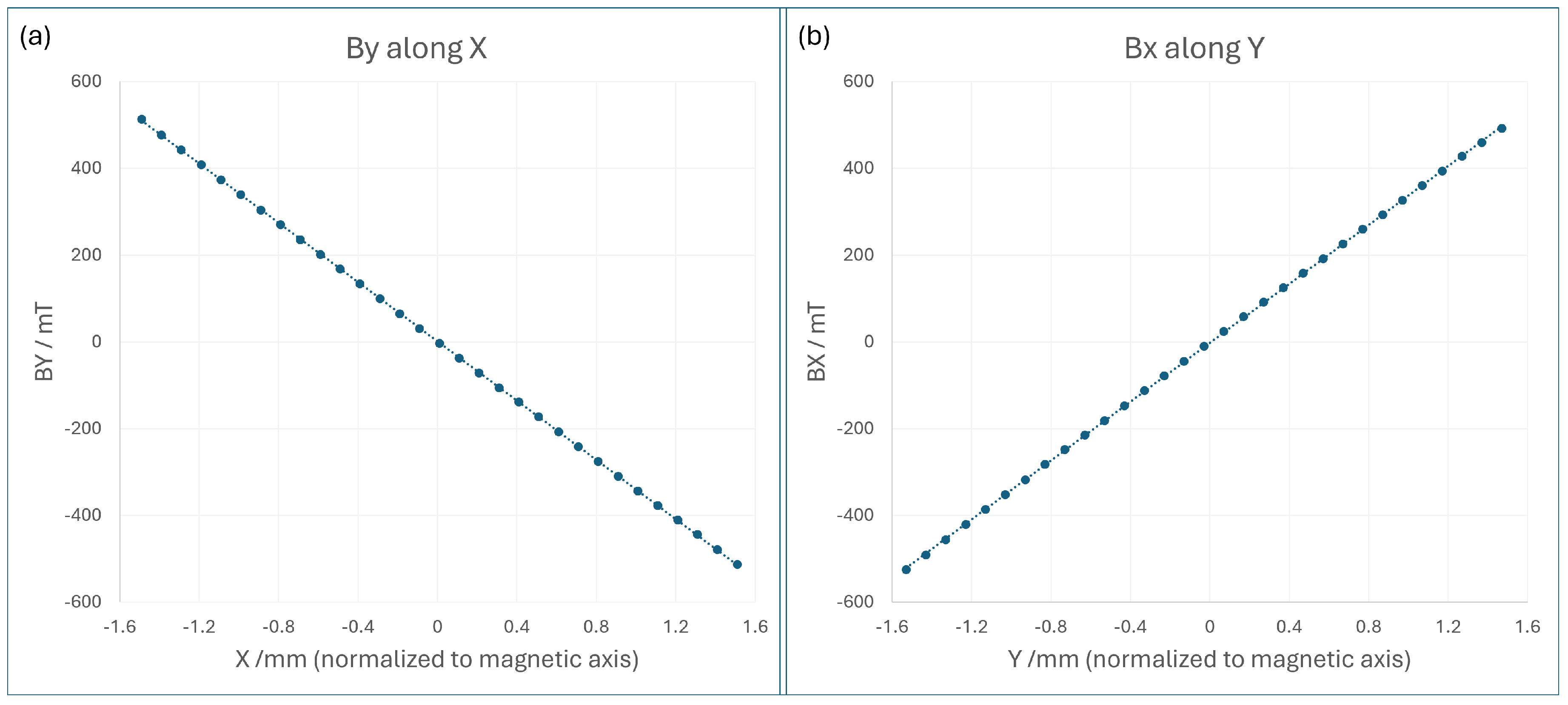
Initially, the probe was placed at the longitudinal centre and scanned in the horizontal and vertical planes until the coordinate of the magnetic centre was approximately located. The probe was then scanned in the horizontal transverse axis (X) and then the vertical transverse axis (Y), with both scans centred about that point. The results are shown in Figure 3.

The measurements showed that a gradient of 340 T/m was achieved, far below the Opera 2D prediction. The sweep distance is limited by the size of the probe relative to the size of the aperture, and finding the gradient and central axis of a quadrupole with a Hall probe is well known to be difficult. However, the scale of the difference was immediately indicative of a severe flaw.

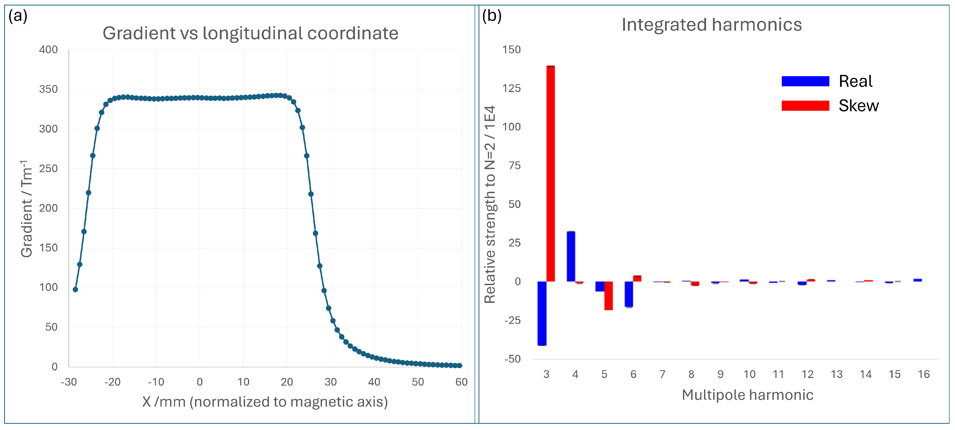
Following the initial straight sweeps of the Hall probe, the measurement was verified by circular sweeps with a radius of 1.5 mm at multiple longitudinal positions, measuring the magnet harmonics and calculating the gradient from a multipole analysis. The field was clearly measured to be quadrupolar in nature, suggesting that the issue could not have been caused by a block being inserted with inverted polarity, with the $n=2$ component clearly dominant. It was possible to extend the probe through the whole magnet but not to measure part of the fringe field on one side as part of the same sweep due to the limitation of the length of the probe and the size of the probe holder.

The results of this integrated circular sweep are presented in Figure 4. The results for gradient as a function of longitudinal position show good agreement with the linear sweeps in Figure 3, confirming the relatively low strength. The integrated harmonics may be calculated from the data, and these reveal a relatively poor harmonic profile, a phenomenon that is common in Halbach arrays due to variations between magnet blocks. In this case, a significant skew sextupole component was observed, although poor alignment to the bench might have been a factor (due to resource limitations, the magnet was not laser-tracked into place).

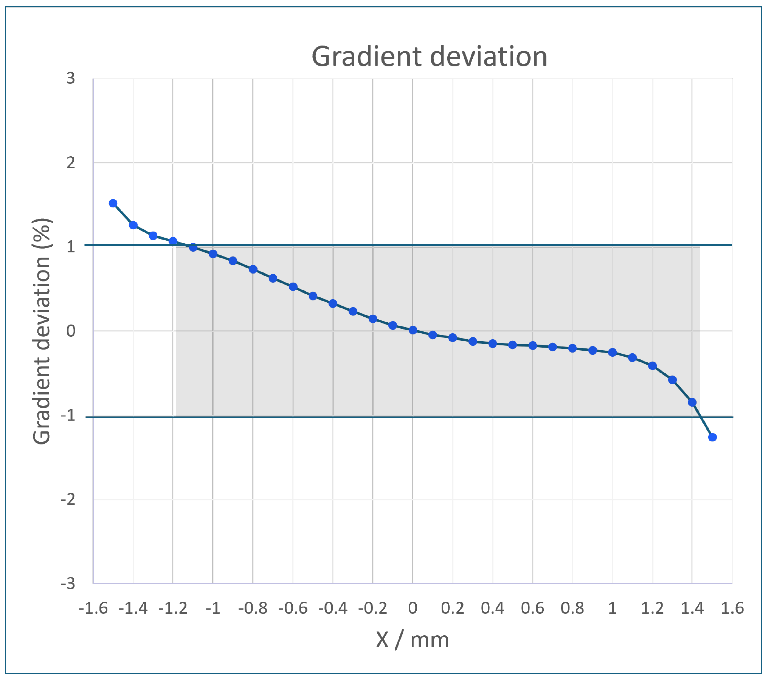
The integrated magnet homogeneity was also measured, again by using the Hall probe. Halbach array quadrupoles have worse homogeneity, in general, than traditional iron-dominated electromagnets with hyperbolic pole tips. However, the use case of EPAC does not demand the high homogeneity specifications of an application like a storage ring. The specification was, therefore, set at a relatively loose ±1 percent for ±1 mm. The measurements of homogeneity are presented in Figure 5, which shows that this specification was achieved for this quadrupole. As simulations and measurements had shown that the homogeneity specification was achievable, corrective measures to shim the magnet were not included in this design.

4. Identifying the Problem

Several avenues of investigation into the discrepancy were pursued. The first question addressed was whether the assembly had been performed correctly. The results of the integrated harmonic measurement, in which the n = 2 component is very dominant, and a visual check of the markings on the magnet blocks both suggested that all blocks were inserted in the correct orientation.

The second step was verifying the calibration of the Hall probe on another known magnet to check for confidence in measurements. The measurements in this case agreed with other measurements on the test magnet and with simulations of the test magnet, suggesting that the Hall probe was functioning correctly.

The third step was to investigate the materials and magnetic permeability of the supporting components (the outer ring and inner support tube). All mounting components were designed to be non-magnetic to avoid short-circuiting of flux. The magnet was disassembled, and a permeability meter (List-Magnetik Ferromaster, Leinfelden-Echterdingen, Germany) was used to check each component, which ruled out the short-circuiting of flux as being the issue.

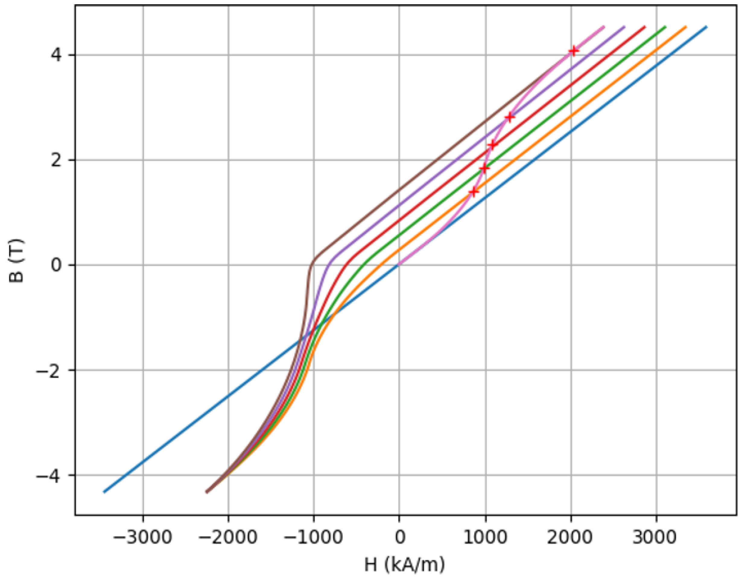
Further investigations were made into the model itself and to the tolerances of the various components. The diameter of the aperture left by the magnet blocks and poles was 9 mm (which reduces to 8 mm with the mechanical support tube). Variations in this were measured, and it was determined that a reduction to 340 T/m would occur if this aperture was increased to 11.8 mm, which was easily ruled out. The steel BH curves were also checked. This design features flux densities up to 3 T in the steel at the narrow end of the steel poles, leading to complete saturation. The Opera simulations account for this with a non-linear simulation applying a BH curve instead of a fixed permeability. To make sure that the steel BH curve was being correctly interpolated beyond its normal range, a repeat of the simulations was performed with a manually specified BH curve in the saturated region. This resulted in no significant changes. The BH curves of the magnet blocks also extended across two quadrants. We had (incorrectly) assumed that this would allow the FEA simulation to account for a reduction in magnetization to a certain extent. The steel and magnet BH curves are shown in Figure 6.

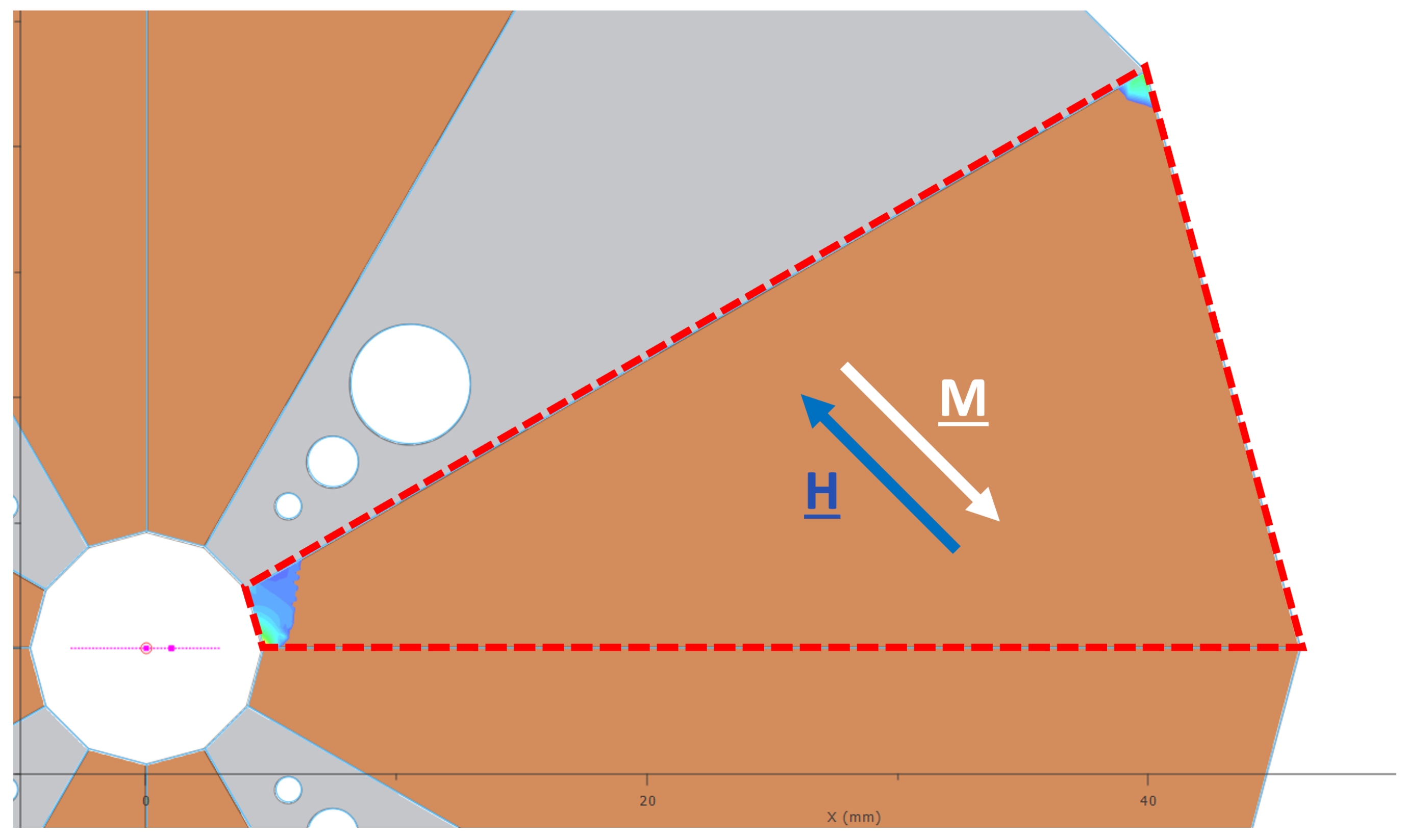
Upon close examination of the Opera 2D and 3D models, it was observed that in the narrow end of the permanent magnet wedges, there was a multi-Tesla field at an oblique angle to the block magnetization. The 3D Opera model with a vector map overlay of this is shown in Figure 7.

The magnitude was above the material coercivity value, and this raised suspicions that although a multi-quadrant BH curve was used in the simulations, demagnetization might have been occurring in the blocks that were not fully accounted for in the simulation. This was investigated further in collaboration with the Opera developers, and it was identified that within the physics model used by the magnetostatic solver code, it would have been impossible for this effect to have been accurately modelled even with the extended BH data. The magnetostatic solver does not record any permanent changes in magnetization of material between iterations; instead, a different solver algorithm was required to model this effect accurately, as discussed in Section 6.

The demagnetization effects can be defined as shown in Figure 8. In this case, the magnet block is magnetized at −45 degrees. The H field opposing the direction of magnetization within the magnet block is $H_{opp}=\underline{H}.\underline{-m}$, where $\underline{m}$ is the unit vector in the direction of the magnetization M. We can take $\underline{m}=\sqrt{2}[1,-1]/2$; therefore,

$$H_{opp}=\underline{H}.\underline{-m}=0.707H_y-0.707H_x$$

(1)

which is the quantity shown in the contour map in Figure 8 exclusively in the region inside the dashed red outline where $H_{opp}\ge H_{cj}$, $H_{cj}$ being the intrinsic magnetic coercivity of VACODYM-745-TP (taken as 1115 kA/m from data available from Vacuumschmelze). Where an opposing field vector is equal to the intrinsic coercivity, a permanent demagnetization is inevitable. Partial demagnetization can occur as the value is approached, and where the value is exceeded, those regions of the block are not only demagnetized, they are also partially re-magnetized along the new field vector. Figure 8 clearly shows this happening in a localized region at the thin end of the magnet wedge, which was neither spotted as a cause for concern in the original modelling, nor does it appear that Opera actually took this effect into account in its predictions of the field gradient in the quadrupole.

5. Measurements of Demagnetization in the Permanent Magnets

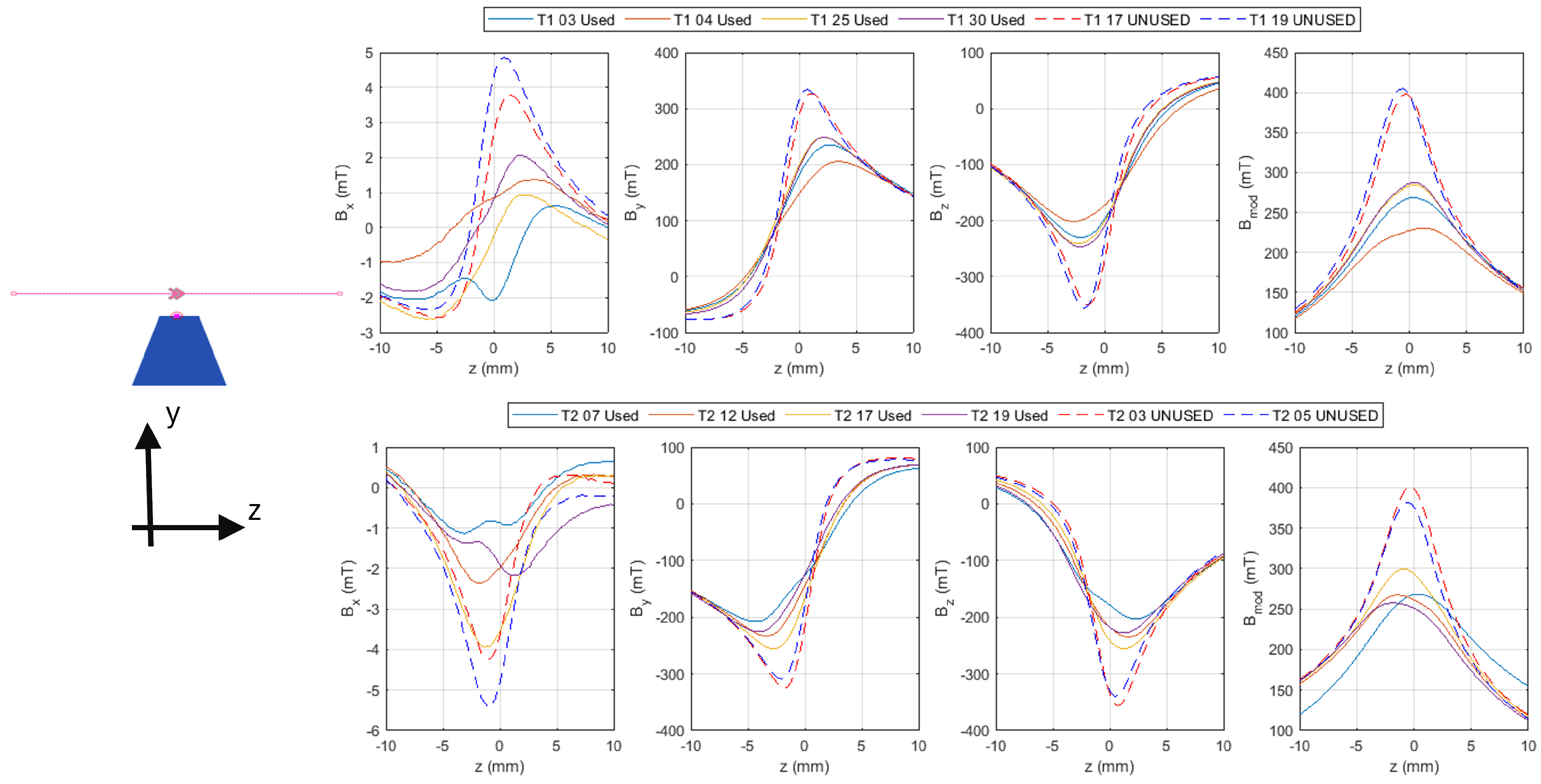
When demagnetization of the permanent magnets near the tips of the wedges was identified as a possible cause, all eight magnet blocks were removed from the magnet and measured individually, as were two unused blocks of each type to act as a comparative reference. This was performed by positioning the blocks with the thin end of the wedge pointing vertically upwards and scanning a Hall probe across the tip, 2 mm above the surface. This method was chosen as it provides more information regarding the local demagnetization of a particular region of the magnet block, as opposed to the more usual method of moving the block in a set of Helmholtz coils to measure overall magnetization.

The results of these scans, as shown in Figure 9, reveal a remarkably consistent pattern. The unused blocks show a distinct peak in the field profile that matches the expected performance, albeit with some variance due to the tolerances on the magnet block’s BH curve and magnetization angle. However, every single used block shows decreased performance relative to the unused blocks, with a significantly weaker peak field measured. The fact that this result is so consistent for every used block is a clear indicator that the demagnetization that may be suspected from the reverse flux vectors shown in the modelling is indeed occurring. It also indicates that the problem is not due to the insertion order of the blocks (in which case stronger effects in certain blocks would be observed); rather, it is a fundamental issue with the design of the magnet itself. The properties of the unused blocks were within specification, indicating that there was no inherent problem with the blocks as manufactured.

6. Replicating the Measurements in Simulation

With the demagnetizing effects proven by measurement, attempts were made to replicate this effect in simulation. A series of models were solved in 2D (again with the magnetostatic solver) with varying amounts of material near the tips of the wedges being replaced with air. The model nominally predicted a gradient of 485 T/m; replacing the material to a 1 mm depth from the thin end of every wedge lowered this to 430 T/m. Replacing 2 mm of material lowered the gradient further to 389 T/m, 3 mm of material to 358 T/m, and 4 mm of material to 335 T/m. This indicates that to replicate the observed 340 T/m gradient approximately, 3.8 mm of material near the thin end of each magnet block would need to be completely demagnetized. In reality, the demagnetization profile is not so simple; however, judging by Figure 8, this may be a reasonable approximation for what is actually occurring.

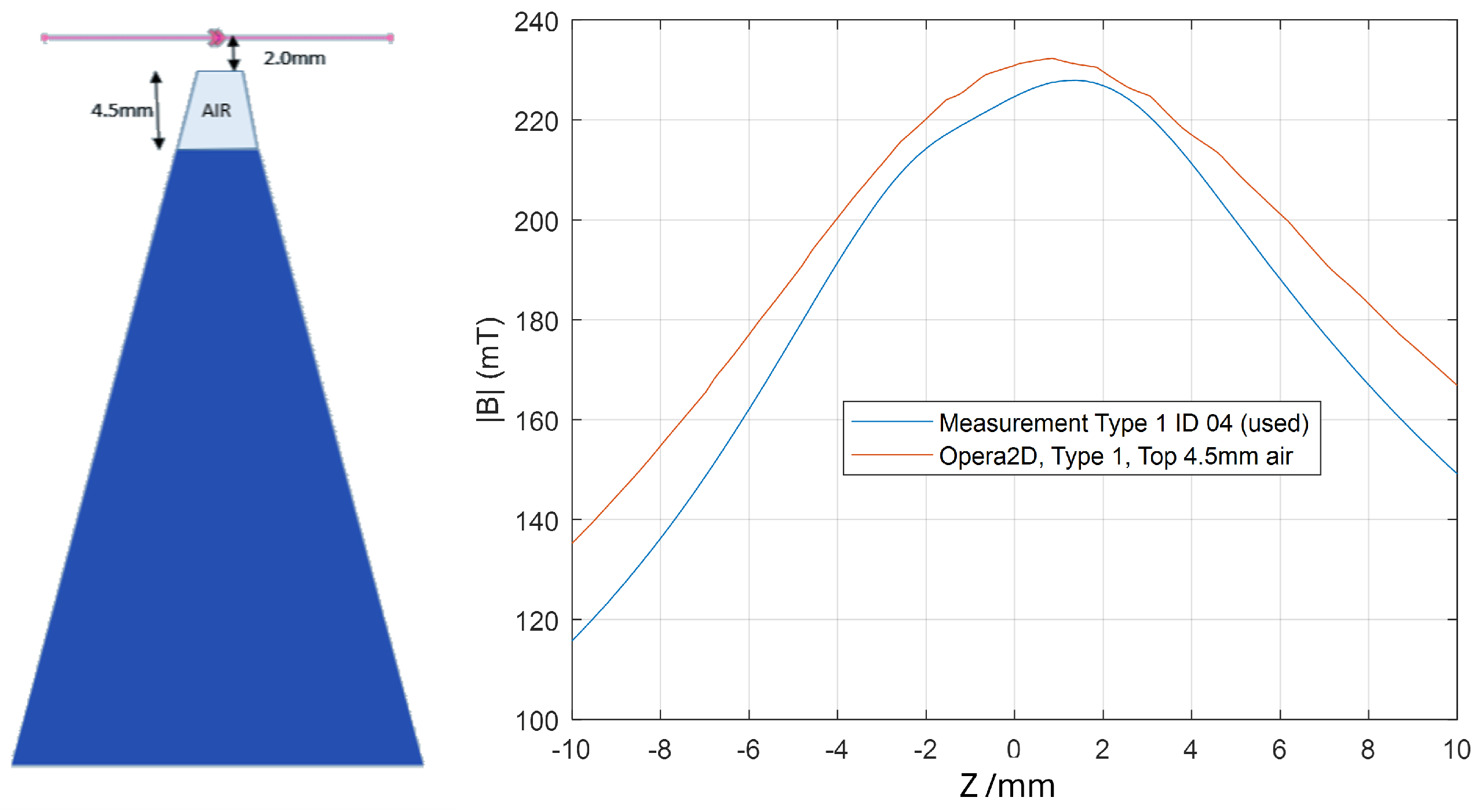
To investigate this further, a single magnet block was modelled in Opera 2D with varying amounts of material at the thin end of the wedge replaced with air to approximate material being demagnetized. It was found that replacing 4.5 mm of material was a good approximation to the actual degradation on performance of the magnet blocks, albeit the actual degradation had some slight block-to-block variance. The comparison between this model and the measurements of one of the used blocks (T1 04) is shown in Figure 10. Over the tip of the block, at $z=0$, the degradation is 3.5%.

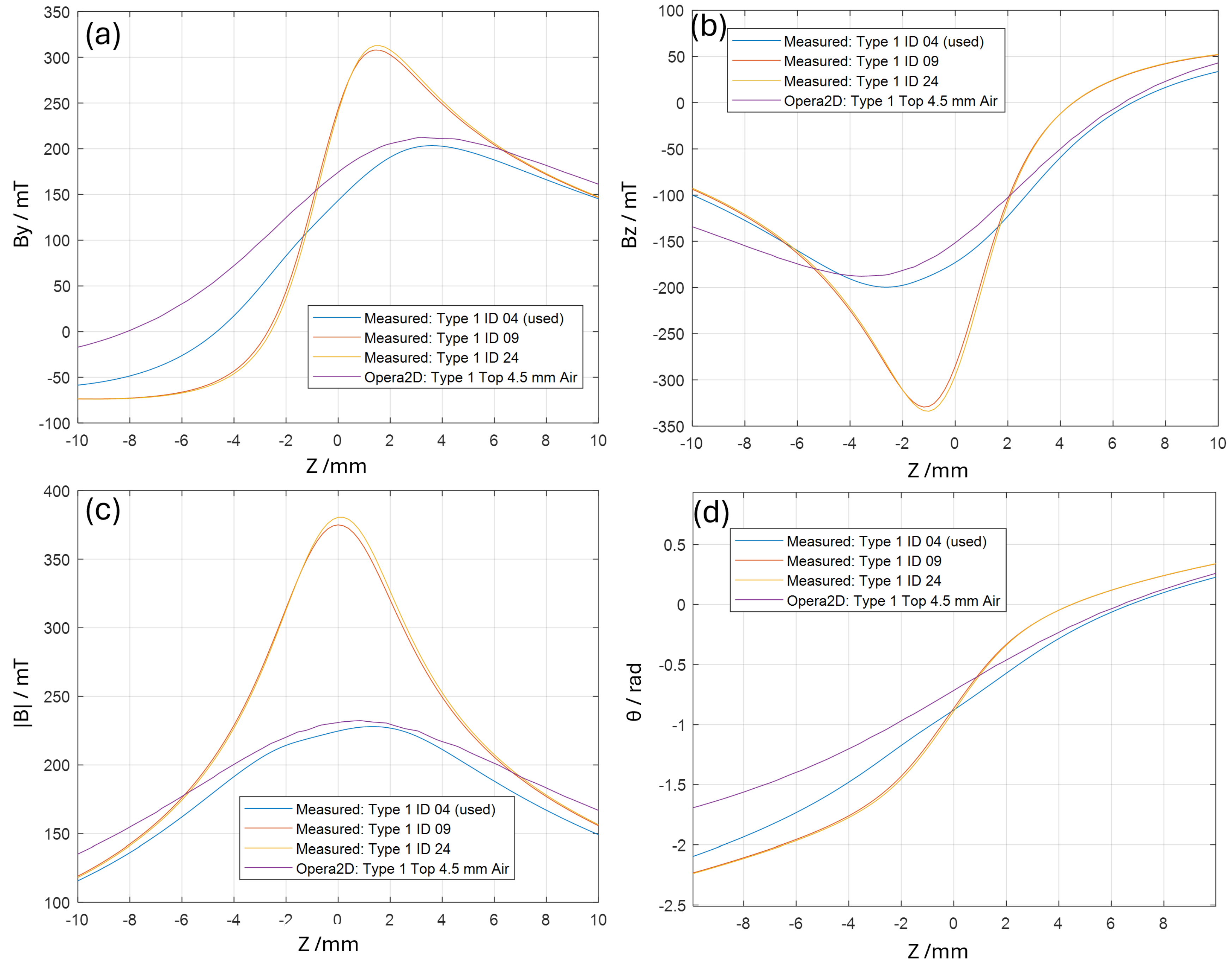
This is explored in further detail in Figure 11, in which $B_z$, $B_y$, $\left|B\right|$, and magnetization angle $\theta$ data from the used block and “matching” Opera model are compared to measured data from two unused blocks. The two unused blocks shown in Figure 11 were measured in the same manner by scanning the Hall probe over the individual blocks as for the data shown in Figure 9. This clearly shows that the demagnetization near the tips of the blocks is a highly viable explanation for the far lower than expected gradient of the quadrupole magnet.

Once we had become aware that demagnetization was occurring, efforts were made to modify the simulations to properly account for the permanent demagnetization effects, in conjunction with Dassault Systemes. This resulted in a technique being devised for simulating these effects more accurately in Opera. Ordinarily, a full simulation that can account for both demagnetization effects and local re-magnetization in a new direction would require magnetization data over the whole hysteresis loop, which were not available to us for the magnet material used. When these data are available, the Opera magnetization solver can be applied to the model, which will allow for local changes in material magnetization at each mesh point of the model to be calculated and stored between iterations.

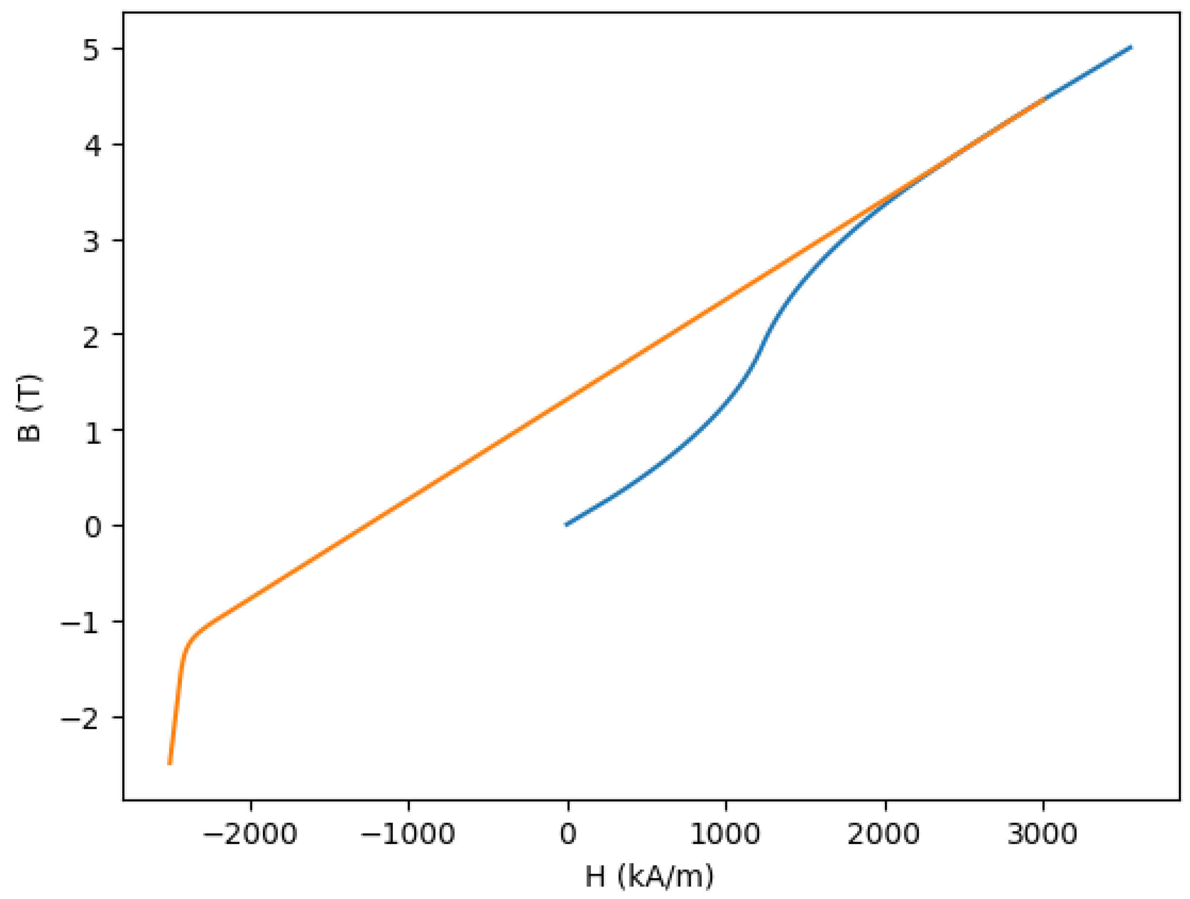
What was available from the manufacturer was the standard 2nd quadrant BH curve for the magnet. This is effectively the magnetization outer loop, but only defined in the 2nd quadrant. This curve was nearly linear at the $H=0$ axis, so it could simply be extended up to saturation in the first quadrant. An ideal virgin curve could then be created, starting from $B=H=0$ and extending up to join the outer loop at saturation. The exact shape of the virgin curve does not precisely matter for this type of simulation. These two plots are shown in Figure 12.

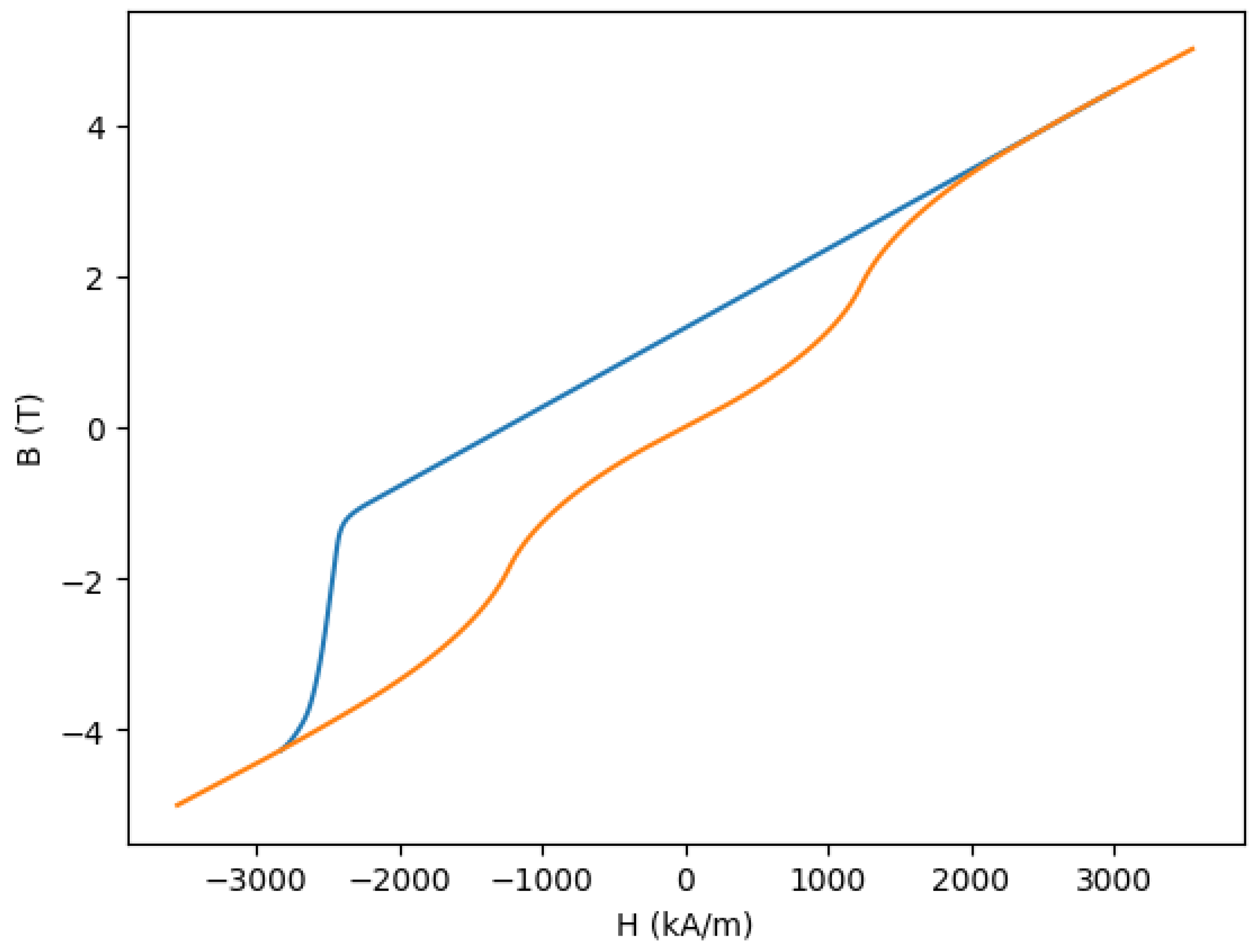
As the material was, in some cases, completely demagnetized, it was also important to extend the outer loop beyond its end in the 3rd quadrant. As there were no measured data available, an approach to extrapolate between known physical limits was used, i.e., between the outer loop end and then to smoothly join the negative of the virgin curve in the 3rd quadrant. This was performed, and the result can be seen in Figure 13.

We then algorithmically generated a series of “interpolated curves” between the outer loop curve and the virgin curve. These curves are what Opera uses to interpolate the magnetization function used for this process. Figure 14 shows the curves used to achieve this. We assumed that the magnet pieces had been fully magnetized to a specific value in the factory, so the history for each element would begin at that value. Thereafter, each element would follow its own trajectory on a magnetization function between that point on the virgin curve and a minimum observed field in the other direction. If this minimum point went past the “knee” or curve of the magnetization function, the element would then recoil to a lower place in the hysteresis diagram. If the element saw a larger field than that used as the starting point for the simulation, its history would be reset and that field would define a new magnetization and direction.

The curves in Figure 14 were produced by a set of python scripts produced by Dassault Systemes, which are included in the Supplementary Information. A typical BH curve for a magnetic material is provided to the script, which then derives an approximate virgin curve followed by several interpolations based on the virgin curve and the original BH curves, and then it exports the data as a table file in a format readable by the Opera software.

After these adjustments were implemented to the simulation, Opera predicted that the same geometry as previously simulated would produce a field gradient of 350 T/m, much closer to the measured 340 T/m than the original prediction of 480 T/m. Whilst this is not a perfect match, it does indicate that this simulation technique is indeed capable of accounting for local demagnetization in a way that agrees broadly with measurement. The fact that it is not a perfect match is likely due to there being some inherent inaccuracies in extrapolating unknown magnetization data into the third quadrant. We believe that if the magnetization table file provided to the simulation had instead contained measured data for the material across the whole hysteresis loop, rather than extrapolated data, the simulation would be an even more accurate representation of reality.

7. Rebuild and Measurement of Further Demagnetization

After the presence of demagnetization effects was confirmed by the work above, the quadrupole was rebuilt. Alongside the process detailed above, the steel poles had been sent for annealing in case machining the tuning holes had changed their magnetic properties, and the aim was to test this. When the quadrupole was re-assembled and re-measured to check this, it was found that the gradient had reduced further to 300 T/m.

A probable cause for this was quickly identified. During assembly, human error resulted in two blocks being inserted in reverse orientation. This was noticed shortly after assembly was completed when a first attempt at measurement yielded unexpected results, triggering a visual inspection of the magnet including the block markings. These two blocks were then removed and re-inserted correctly. However, during the incorrect insertion, these two blocks were exposed to strong fields from the neighbouring blocks in opposition to their magnetization vector, which likely demagnetized them further, as well as affecting the neighbouring blocks. 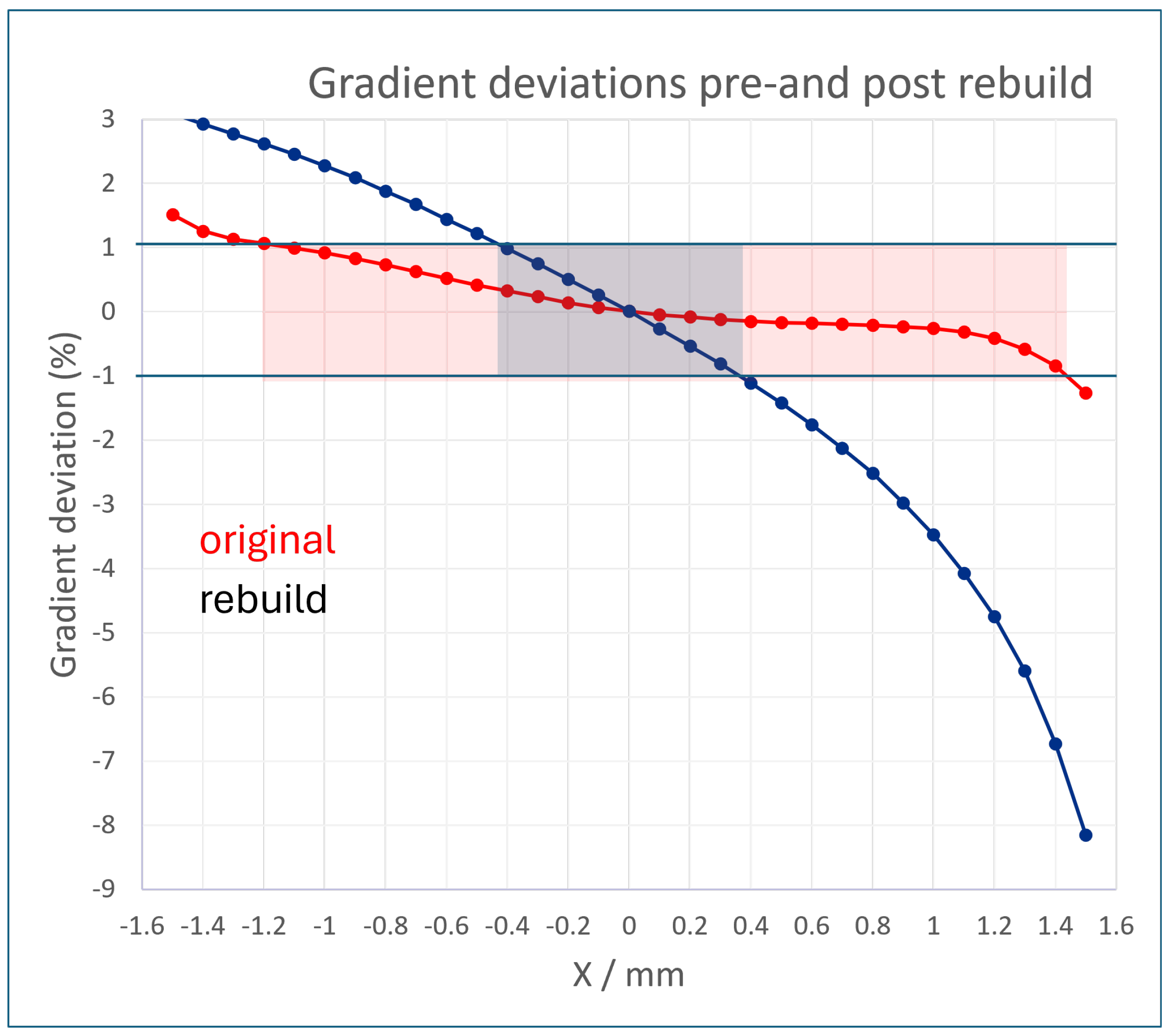Rather than flux feeding from one block into another as per Figure 1, the magnetization vectors would have pushed flux at an orthogonal angle to the magnetization vector near the joint between the blocks, resulting in local demagnetization followed by re-magnetization in that new orthogonal direction. Following the rebuild, a severe degradation in gradient homogeneity was also observed, even after the mistake in block positioning was corrected. This indicated that the incorrectly inserted blocks did indeed experience further permanent degradation. Even with correct assembly, the magnetization of the quadrupole was no longer symmetric, resulting in the severely affected gradient homogeneity. The measurement of this is shown in Figure 15.

It can be clearly seen that even the relatively loose ±1 percent for ±1 mm homogeneity target was no longer achieved, and the gradient homogeneity transitioned from a slight but acceptable asymmetry to an extreme and unusable asymmetry. The asymmetry indicates that blocks on one side of the magnet were demagnetized more than the other side, suggesting permanent damage caused by incorrect insertion of magnet blocks. This result highlights the importance of a rigorous assembly procedure.

8. Conclusions and Outlook

We built a new hybrid Halbach array permanent magnet quadrupole for the EPAC project, which is designed to capture a broadband multi-GeV electron beam from a laser-plasma source. The design features an innovative tuning pin arrangement to compensate for reasonable variations in strength. The hybrid Halbach array design, combined with the combination of an unusually high strength and unusually large aperture for such a design, leads to flux vectors near the magnet block tips opposing the magnetization direction of the blocks.

When the design was measured, the strength was significantly lower than anticipated due to this demagnetization effect. Extensive measurements of the removed magnet blocks confirmed localized demagnetization near the thin ends of the magnet wedges that was not predicted by the magnetostatic solver of the Opera FEA software used for the initial design. After this was identified, a technique was developed to allow Opera to derive a virgin BH curve and a set of interpolated curves from the limited BH information available for the magnet material. This technique allowed for the generation of a table of magnetization data, which allowed the simulation to take this localized demagnetization effect into account by applying a magnetization solver to the model and, thus, enabled the simulation to more accurately predict the true magnetic field produced by the magnet blocks. This indicated that we had successfully integrated measurement and simulation to understand how this effect occurred.

The work here highlights a risk present in hybrid Halbach array quadrupoles, which only manifests when highly saturated, that designers and assembly technicians should be wary of. We present this as a warning, in particular that designers should inspect their models for potential demagnetization effects properly and should modify their models to simulate these effects if the potential for demagnetization is suspected. We provide here a potential technique for doing so. It also highlights the need for rigorous assembly protocols to avoid further accidental demagnetization.

For future designs, reducing pole tip fields is the obvious solution. However, in the case of EPAC, the strength and aperture combination is dependent on too many other factors to be allowed to be compromised. As the possibility of this effect occurring was not considered during design, VACODYM-745-TP was chosen as the magnet material due to its high remanence, despite it having a relatively low intrinsic coercivity specification. Higher coercivity PM materials are available, and using them is a viable solution albeit at the cost of lower remanence. For example, material grade VACODYM-806-TP has a $H_{cj}$ of −1990 kA/m and a $B_r$ of 1.3 Tesla and so may be appropriate, although it would require a larger volume of material to achieve the required strength. Alternatively, materials that have undergone grain boundary diffusion are also more resistant to demagnetization but are only effective in certain aspect ratios.

Alternatively, designing the magnet such that the end face of the wedges is set back from the end face of the steel pole tips may reduce the presence of reverse flux vectors in the magnet material; this has been observed before in hybrid permanent magnet undulators [22,23].