Evaluation of Image Segmentation Methods for In Situ Quality Assessment in Additive Manufacturing

Abstract

Additive manufacturing (AM), or 3D printing, has revolutionized the fabrication of complex parts, but assessing their quality remains a challenge. Quality assessment, especially for the interior part geometry, relies on post-print inspection techniques unsuitable for real-time in situ analysis. Vision-based approaches could be employed to capture images of any layer during fabrication, and then segmentation methods could be used to identify in-layer features in order to establish dimensional conformity and detect defects for in situ evaluation of the overall part quality. This research evaluated five image segmentation methods (simple thresholding, adaptive thresholding, Sobel edge detector, Canny edge detector, and watershed transform) on the same platform for their effectiveness in isolating and identifying features in 3D-printed layers under different contrast conditions for in situ quality assessment. The performance metrics used are accuracy, precision, recall, and the Jaccard index. The experimental set-up is based on an open-frame fused filament fabrication printer augmented with a vision system. The control system software for printing and imaging (acquisition and processing) was custom developed in Python running on a Raspberry Pi. Most of the segmentation methods reliably segmented the external geometry and high-contrast internal features. The simple thresholding, Canny edge detector, and watershed transform methods did not perform well with low-contrast parts and could not reliably segment internal features when the previous layer was visible. The adaptive thresholding and Sobel edge detector methods segmented high- and low-contrast features. However, the segmentation outputs were heavily affected by textural and image noise. The research identified factors affecting the performance and limitations of these segmentation methods and contributing to the broader effort of improving in situ quality assessment in AM, such as automatic dimensional analysis of internal and external features and the overall geometry.

1. Introduction

Feature recognition serves as an important factor in ensuring quality control in additive manufacturing (AM), a process of fabricating components layer by layer from digital models. Advancements in AM have led to the ability to fabricate increasingly complex components with intricate geometric features, complex material compositions, and a variety of surface textures. The quality of an AM part is often dependent on its conformance with predefined specifications and performance requirements, making the role of part feature recognition at the layer level indispensable. In addition to the external part geometry and features, the internal features of an AM part, such as channels, cavities, and support structures, can significantly impact the function, performance, and reliability of the printed part for its intended application. Defects or irregularities in these features, such as the geometry, location, voids, cracks, or unwanted material accumulations, can lead to possibly reduced performance and potential failure of the printed part. Hence, recognizing and accurately segmenting these features on a layer becomes an essential first step for ensuring the quality of the final part and identifying potential manufacturing defects or irregularities during the fabrication process.

Traditionally, quality control methods have relied on post-processing inspections using X-ray computer tomography (XCT) [1,2,3] and ultrasound imaging [4,5] to obtain information about the internal features of a printed part. For example, Reider et al. [4] used ultrasound to perform non-destructive testing (NDT) on selective laser melting (SLM) parts to detect internal stresses and porosity. Petruse et al. [6] investigated how different slicing approaches and printing parameters affect the dimensional accuracy of parts manufactured using fused deposition manufacturing (FDM) with a FARO Edge measuring arm. However, these approaches are only employed after the part is fully fabricated and possibly removed from the build platform, thus making it difficult to detect any deviations from the design specifications during the fabrication process, especially for a part’s interior geometry and features. Moreover, these methods are time-consuming, expensive, and require specialized equipment, making them unsuitable for real-time defect detection during the manufacturing process.

As such, there has been growing interest in exploring automated methods which complement traditional inspections by leveraging advancements in digital image processing and computer vision approaches to perform in situ quality control during AM process [7,8,9,10,11]. Image segmentation, a process in the computer vision and image processing domains, is employed to isolate and identify features of interest within an image. It offers an easy to implement and cost-effective solution for enhanced feature recognition through boundary detection and differentiation of areas within an image. In AM, segmentation can be used to identify the edges of the internal and external geometry and detect defects in a part. The effectiveness of the segmentation method depends on environmental, process, and imaging factors [9]. Environment factors such as lighting and any unwanted shadows can result in bright and dark spots on an image. Variations in process parameters such as the extrusion speed, extrusion width, and temperature can affect the material deposition process and introduce ridges and gaps in the surface texture of the printed layer. The complexity of the printed part due to the presence of internal features and voids and the infill direction can also affect the segmentation output. Additionally, imaging factors such as the camera resolution, focal length, and camera-part distance and image processing properties such as contrast, brightness, and noise can affect the quality of a captured image. In the literature review section, applications of segmentation to identify features and defects are discussed. However, no studies evaluating the performance of different segmentation methods for feature identification in AM have been identified. Also, in order to perform a proper and non-biased comparison of the segmentation methods considered, it is important to ensure that the experimental results are not biased by external factors such as the manufacturing or printing environment and platform, part geometry, or imaging process.

In this research, a number of segmentation methods are evaluated to assess their applicability in identifying the external geometry and internal features in an AM part. These methods are evaluated using images of AM parts obtained in situ by comparing their ability to segment features correctly and their tolerance toward noise within images under different lighting and contrast conditions. The comparison of these methods will allow the evaluation of their performance toward providing accurate feature segmentation within AM parts. The results of this research could serve as an important step toward enhancing existing quality control measures by integrating automated in situ layer-by-layer feature recognition.

In this article, the literature survey is discussed in Section 2, highlighting commonly used methods for quality control in AM and the use of imaging methods for feature recognition. The image segmentation and processing methods used in this research are introduced in Section 3. The experimental set-up we developed and employed is presented in Section 3.5. The research results are presented and discussed in Section 4 and Section 5, respectively. The article closes with conclusions and recommendations for future work.

2. Literature Survey

Quality control in AM is an important aspect of the manufacturing process for ensuring the final product meets the defined specifications and performance requirements. However, ensuring high-quality manufactured parts has remained a challenge, which reinforces the need for advanced process monitoring methods. Several researchers and industries have developed in situ monitoring technologies using machine vision and other sensor-based frameworks to address the challenges of ensuring high-quality AM components and reduce manufacturing failure rates.

Closed-loop control systems for AM processes have been developed to improve specific part properties or rectify errors during the print process itself. Garanger et al. [12] developed an in situ feedback control scheme based on stiffness measurements taken during the process to achieve the desired stiffness by adjusting the infill density. Cummings et al. [13] presented a closed-loop system based on ultrasonic sensing to detect and correct filament bonding failures. These systems adapt and adjust controllable process parameters such as the feedrate and extruder and bed temperature to mitigate issues associated with filament bonding failures, highlighting an evolved approach toward autonomous quality control in AM.

Digital twins (DTs) in AM processes, especially within metal printing domains such as laser powder bed fusion (LPBF) and directed energy deposition (DED), signify a shift toward merging physical printing processes with their digital counterparts for enhanced monitoring and control. Gaikwad et al. [14] explored incorporating physics-based predictions with machine learning algorithms to forecast defects and process irregularities in metal additive manufacturing. Their results showed significant improvements in predictive accuracy for temperature distributions and flaw detection when combining graph theory-based models with sensor data. Knapp et al. [15] highlighted the integral role of monitoring parameters such as temperature gradients and cooling rates via DT technology to ensure part quality. Nath and Mahdevan [16] discussed the optimization and control of a manufacturing process, using a DT approach to monitor the melt pool with a thermal camera to predict the quality of manufactured parts and adjust the laser power in real time.

Machine vision technologies have been extensively studied for quality control in AM processes. Generally, cameras have been used to capture an image of a part after it has been printed, which is then analyzed to detect external defects or irregularities [7,9,17,18]. Image thresholding is commonly used to distinguish the image of a printed part from the background by generating a binary mask of the printed part. Anomaly detection is then performed by either employing differential imaging approaches across consecutive frames of the same part [17], by comparing the generated mask with reference masks from successfully completed parts [7], or by comparing it with a synthetically created mask produced using a computer-aided design (CAD) model [9,18]. However, these approaches can only identify the external part features and geometry after a part has been printed.

Machine vision systems have been used to monitor the material deposition of the fused filament fabrication (FFF) process by mounting a camera close to the dispensing nozzle. Liu et al. [8] mounted a camera on the print head to capture images of a part as it is being printed to optimize the deposition parameters and observe the surface texture of the layer. Images are captured either from the top to analyze the layer surface texture for in-layer defects [8,19] or from the side to detect external defects such as layer delamination [20,21].

Another printing process monitoring approach is to observe the printed layer from above using optical sensors, which allows for capturing and analyzing images of a printed layer in real time [20,22,23,24,25]. Khan et al. [22] presented a deep learning model based on a convolutional neural network (CNN) to detect geometric distortions in infill patterns and classify printed objects in real time as ‘good’ or ‘bad’. He et al. [23] and Yi et al. [24] used image segmentation information based on thresholding to develop statistical process methods and monitor the external geometry of a printed layer. Delli et al. [25] and Shen et al. [20] used machine learning algorithms to train models using multiple thresholding-based images to differentiate between successful and failed layers. Instead of studying the whole layer, research focused on smaller regions of the layer, where the imaged regions were classified as ‘in control’ or ‘out of control’ [10,11]. Rossi et al. [10] compared the performance of different binary classifiers for image patches, but the output of such classifiers did not contain segmented features. Moretti et al. [11] used Canny edge detection segmentation to identify the external boundary of a printed part in a layer-by-layer process.

Three dimensional (3D) imaging approaches such as photogrammetry and laser line scanning have also been explored. Photogrammetry captures images of a printed part from multiple angles and then uses triangulation to reconstruct the 3D model of the printed part. This method has been used to detect defects in parts such as warping, delamination, and surface roughness [26,27]. Nuchitprasitchai et al. [26] used photogrammetry with six cameras to detect print deviations due to a clogged nozzle or filament loss by comparing the point cloud to the CAD model. Holzmond and Li [27] described a method to detect defects in parts produced by the FFF process using a two-camera 3D digital image correlation (3D-DIC) set-up. The 3D-DIC method uses the natural speckle pattern of the material to generate point clouds of the printed layer. In laser line scanning, a thin fringe pattern is projected onto the part. The surface geometry is captured using two cameras and analyzed to detect surface defects such as under-extrusion and over-extrusion [28]. While 3D imaging methods provide a more comprehensive view of the part, they are more complex to implement compared with 2D imaging methods due to the large amounts of image data which need to be processed and analyzed.

Segmentation methods have found applications in diverse areas outside the field of AM. Grand-Brochier et al. [29] compared the performance of several segmentation methods, such as thresholding, edge detection, region growing, and clustering, in segmenting tree leaves from natural backgrounds. The performance of these methods was evaluated using several criteria, such as accuracy, precision, and the Jaccard index. Marcomini et al. [30] evaluated the effectiveness of Open Source Computer Vision Library (OpenCV)-based segmentation methods for their ability to segment and detect vehicles in highway traffic videos. Ng et al. [31] and Huang and Chen [32] used the watershed transform method to segment and detect tumors in medical resonance imaging (MRI) images. Ajai and Gopalan [33] compared the performance of the Sobel edge detector method with other traditional edge detection algorithms to detect tumors in brain MRI images. These comparative analyses and evaluations reinforce the importance of selecting appropriate methods to achieve improved segmentation performance based on the application, features of interest, and characteristics of the captured image.

Several studies used edge detection and thresholding methods to detect the external geometry of a printed part and the presence of defects on the printed surface. Additional methods such as Sobel edge detection and the watershed transform were investigated, since they have been widely used in segmenting tumors in medical scans [31,32,33]. These methods rely on a strong contrast between the part and the background to detect the features of interest. However, in AM parts in general, and especially in FFF parts, the internal features might not be easily distinguishable from the background since the last printed layer is usually visible through the current layer. While machine vision technologies have been widely used to identify features and defects, there are no studies which compare the performance of various segmentation methods for AM, especially for multi-layer scenarios with varied contrast levels using the same printing and imaging environments and the same parts and features in situ.

3. Methods and Materials

Accurate identification and recognition of the external geometry, surface defects, and internal features is important to ensure the quality of the part being manufactured. This identification and recognition process is performed by examining and analyzing the part at various stages of production to detect any deviations from the as-processed and eventually the as-designed part. In AM processes, this examination could be performed in situ on a layer-by-layer basis to ensure that each layer conforms to the processed print file specifications, which are generated based on the CAD model of the designed part and the printing process.

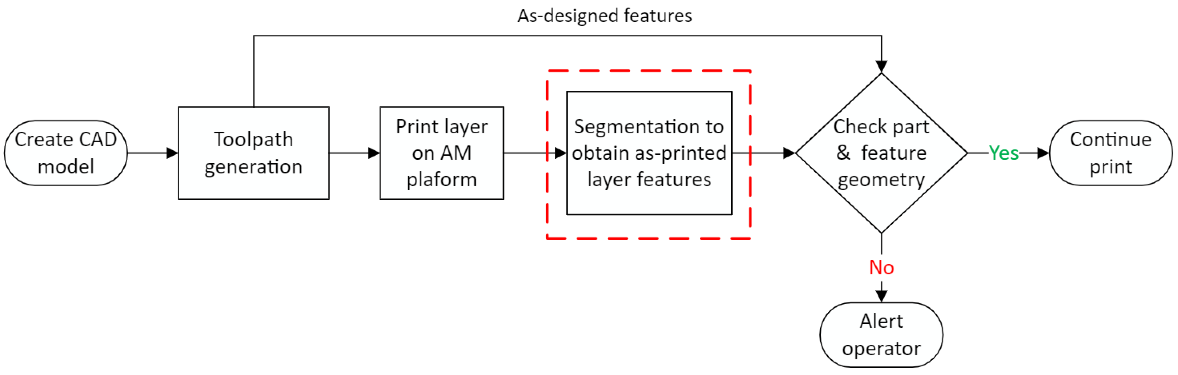
Saini and Shiakolas [34] proposed and demonstrated an in situ vision-based methodology using segmentation to detect the geometry and shape of the external boundary and internal features on the first layer of an FFF-printed part as shown in Figure 1. They used a camera to capture images of the printed layer, which were processed to identify the features of interest. The detected features were then compared to the as-processed layer information obtained from the geometric code (G-Code) to assess the dimensional conformity of the printed layer.

An important step in this methodology is the segmentation procedure. The effectiveness of the segmentation method used can significantly impact the accuracy and reliability of the feature recognition system. The segmentation procedure isolates and identifies the features of interest in the image and can be performed using various image processing techniques.

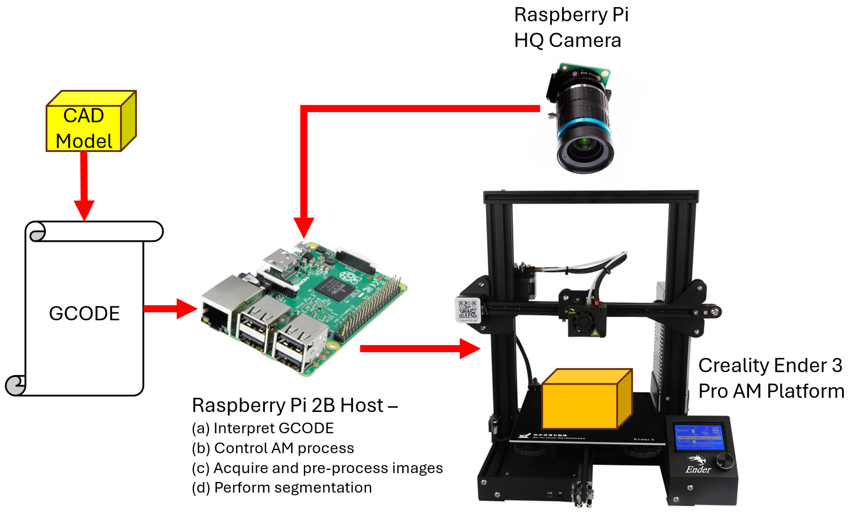
The methodology is built around a computing device or host (Raspberry Pi) which interprets the processed part’s G-Code (generated from the exported part CAD model) and controls the AM and imaging processes. The host coordinates the image acquisition process using a camera (Raspberry Pi HQ Camera) to capture top-view images of the most recent printed layer. These images are then processed and segmented to identify internal and external features. The flow of information between the various components is shown in Figure 2.

Based on the literature survey, a number of image segmentation methods popular in the field of image processing were identified to evaluate their performance for potential application to feature recognition for AM. These methods were simple thresholding, adaptive thresholding, Sobel edge detection, Canny edge detection, and the watershed transform. A brief overview of each method introduces its principle of operation along with advantages and limitations.

The segmentation methods were implemented in the Python programming language using OpenCV [35]. OpenCV is an open-source computer vision and machine learning software library which includes a comprehensive set of computer vision algorithms. The performance of each segmentation method was evaluated using images of AM parts obtained in situ by calculating the accuracy, precision, recall, and Jaccard index metrics, as they apply to detecting and identifying internal features on different layers of a part.

3.1. Thresholding

Simple and adaptive thresholding are two common approaches used in the field of image segmentation and feature recognition. Both methods use the ‘threshold’ criterion to divide an image’s pixels into two groups: the foreground and background. The threshold value is applied to the image either globally (simple thresholding) or by dynamically adjusting the threshold based on the local image properties (adaptive thresholding). A detailed overview of each method is provided, highlighting its principle of operation, advantages, and limitations.

3.1.1. Simple Thresholding

Simple thresholding [36,37] is an image segmentation method where by using the pixel intensity (I), the image of a 3D printed geometry (foreground) can be separated from the background (usually with a different pixel intensity).

An optimal pixel intensity threshold value is defined by the operator, where any pixel with an intensity on one side of this threshold is interpreted as the printed part while any pixel with an intensity on the other side of the threshold is interpreted as the background (for example, the build platform or the previous layer). The process is mathematically represented by Equation (1), where $T(x,y)$ is the binarized output image after thresholding, t is the threshold value, and $(x,y)$ are the coordinates of the pixel being evaluated:

$$T(x,y)=\left\{\begin{array}{cc}0\hfill & \mathrm{if}I(x,y)<t\Rightarrow \mathrm{foreground}\hfill \\ 1\hfill & \mathrm{if}I(x,y)\ge t\Rightarrow \mathrm{background}\hfill \end{array}\right.$$

(1)

For example, dark-colored 3D printed parts with a bright background will have a pixel intensity below the threshold and background pixels with an intensity above the threshold, whereas the opposite is true for light-colored parts on a dark background. Selecting the right threshold value is critical and generally requires prior knowledge of the distribution of pixel intensities. An overly high value can include undesirable elements such as the texture on the bed, while too low a value may exclude important features. While thresholding is easy to implement and requires low computational resources, it has limited success when segmenting images with low contrast between the printed layer (foreground) and the bed (background). This limitation is more pronounced when segmenting features on multi-layer parts, where in most cases the same colored layer might be visible through ‘hollow’ or ‘void’ printed features. Also, in environments where lighting conditions might not be optimal, shadows or bright spots can lead to the detection of false edges.

3.1.2. Adaptive Thresholding

Simple thresholding requires high contrast between the regions to properly segment them based on a provided threshold. However, components manufactured using AM often do not show a clear difference between internal details because the previous layer might be visible through these features, as they are made from the same material and exhibit a similar pixel intensity.

Adaptive thresholding [38] is used in image processing to convert a grayscale image to a binary image. Unlike simple thresholding, which uses a global threshold value, adaptive thresholding adjusts the threshold value based on the local image properties. A window or a block of pixels is selected to compute the threshold based on the local contrast, making it more effective in varying lighting conditions. The window size determines the local area used, and the threshold value is calculated for each pixel based on the mean or weighted mean of the pixel intensities in the window. This method is commonly used for document scanning and optical character recognition (OCR) applications, since it is able to detect contours under a variety of lighting conditions. Components manufactured using AM often have regions with varying pixel intensities, making adaptive thresholding an appealing choice for feature recognition.

Defining appropriate parameters, such as the correct window size and weights [38], poses a significant challenge for application of the thresholding method. Additionally, adaptive thresholding relies on the assumption that smaller regions within an image have roughly uniform illumination, which may not hold true for complex textured images or those with intricate geometric patterns.

3.2. Edge Detection

Edge detection operates on the principle of identifying areas where the image experiences sudden changes in the pixel intensities, which can be used to segment the ‘edges’ between different features. While edge detection algorithms are able to capture subtle changes in an image, which can help in segmenting soft edges, this ability makes them highly sensitive to image noise. Sobel and Canny are two commonly used edge detection methods.

3.2.1. Sobel Edge Detector

The Sobel edge detector [39], also known as the Sobel filter or Sobel operator, is a type of convolutional mask used primarily in edge detection algorithms. The operator consists of a pair of convolution masks $3\times 3$ in size. One mask is used to detect edges in the horizontal direction, and the other detects edges in the vertical direction. The masks are used to calculate the gradient of image intensity at each pixel within an image. The magnitude of this gradient identifies the edges present in that image. Since this is a gradient-based method, it is highly sensitive to noise and requires noise reduction as a preprocessing step. Also, it does not perform well on curved or diagonal edges due to it inherently being designed for detecting primarily vertical or horizontal changes.

3.2.2. Canny Edge Detector

The Canny edge detector [40] is a multi-stage algorithm designed to detect a wide range of edges in images. The Canny method follows several steps: smoothing the image with a Gaussian filter to reduce noise, finding the intensity gradients, applying non-maximum suppression to remove unwanted responses to edge detection, and using double thresholding to determine potential edges [41]. The Canny edge detector is proficient in detecting sharp edges which have a strong contrast when compared with the background. However, it is limited in its ability to detect weak edges and regions with a gradient or uneven textures. A $9\times 9$ Gaussian filter size was used to reduce background noise. However, some high-frequency noise or texture within images can still be erroneously interpreted as edges, leading to false positives. The Canny edge detector uses global thresholds, which might not work well for images with varying lighting conditions or contrast levels, such as in the case of multi-layer parts, where the previous layer is usually visible through the current layer.

3.3. Watershed Transform

The watershed transform is a region-based method used in image processing to segment images into different regions. The algorithm, originally developed by Digabel and Lantuejoul [42], treats the grayscale image it operates on as a topographic surface, where light areas are considered as peaks (watersheds) and dark areas are considered as valleys (catchment basins). The image is completely decomposed by the watershed transform, and all pixels are assigned to a peak or valley. The methodology simulates flooding the surface from specific seed points located in the valleys and labels areas as they become completely surrounded by water, effectively delineating boundaries between different objects or regions. The approach is highly effective in separating objects in an image with irregular and complex shapes similar to the geometry found in the interior layers of 3D printed parts.

A key challenge with the watershed transform is its tendency to result in oversegmentation, especially in images with noise or texture. This might lead to a single object being divided into many small segments unless preprocessing steps are implemented to minimize this effect. Since watershed segmentation relies on intensity gradients to define boundaries, variations in lighting or contrast within an image can affect its performance. For example, uneven illumination across a 3D printed layer could potentially lead to inaccurate boundary detection.

3.4. Performance Metrics and Their Evaluation

Accuracy, precision, recall, and the Jaccard index are commonly used measures or metrics for evaluating image data to provide insight into the performance of a segmentation method. They can be defined mathematically using the concepts of true positive ($TP$ ), true negative ($TN$), false positive ($FP$), and false negative ($FN$).

Accuracy is a measure of the overall correctness of a classification model. In the context of edge detection in 3D printed models, the accuracy indicates the proportion of true results (both true positive edge detections and true negative non-edge detections) in the total image area. It is evaluated according to Equation (2):

$$\mathrm{Accuracy}={\displaystyle \frac{TP+TN}{TP+FP+TN+FN}}\times 100\%$$

(2)

Precision is the proportion of positive edge detection which actually corresponds to real edges in the ground truth and is evaluated according to Equation (3). A high precision score indicates that a predicted edge is highly likely to be an actual edge. This metric is important for detecting false positives. A high precision value corresponds to a low false positive rate:

$$\mathrm{Precision}={\displaystyle \frac{TP}{TP+FP}}\times 100\%$$

(3)

Recall or sensitivity defines the ability of a method to identify the actual edges from all detected edges. This metric presents the proportion of actual positives (edges in ground truth) correctly identified as shown in Equation (4). A high recall number is desired since this indicates that the segmentation method is effective at detecting as many true edges as possible, thus reducing the likelihood of missing critical features in segmentation:

$$\mathrm{Recall}={\displaystyle \frac{TP}{TP+FN}}\times 100\%$$

(4)

The Jaccard Index or Jaccard similarity coefficient is a statistic used to compare the similarity and diversity of sample sets. It measures the similarity between finite sample sets and is defined as the size of the intersection divided by the size of the union of the sample sets. It is evaluated according to Equation (5):

$$J(A,B)={\displaystyle \frac{|A\cap B|}{|A\cup B|}}$$

(5)

where A and B are the two datasets being compared. Since the datasets are binary images, the Jaccard index (Equation (5)) can also be written as shown in Equation (6):

$$\mathrm{Jaccard}\mathrm{Index}={\displaystyle \frac{TP}{TP+FP+FN}}\times 100\%$$

(6)

When evaluating a segmentation methodology to detect the edges of a 3D printed part, the Jaccard index evaluates the overlap between the predicted segmentation and the ground truth. A higher Jaccard index indicates a closer overlap between the segmentation output and the ground truth, indicating a more accurate segmentation output.

These metrics are used to evaluate the performance of each segmentation method in terms of how accurate its predictions are (accuracy), how reliable its positive predictions are (precision), how well it identifies positive instances (recall), and how similar the segmentation output is to the ground truth (Jaccard index).

3.5. Experimental Set-Up

The performance of the segmentation methods was evaluated using images of 3D printed parts for one, two, and multiple layer scenarios. These images were captured in situ after printing each layer on a Creality Ender 3 Pro 3D printer (Creality, Shenzhen, China) [43], a commercially available FFF platform with a single extruder. An appealing feature of this printer is its open-frame design, which allows for easy customization, especially for the purposes of this research, where an image acquisition set-up was developed and adapted on the extruder assembly to capture images of printed part layers in situ. 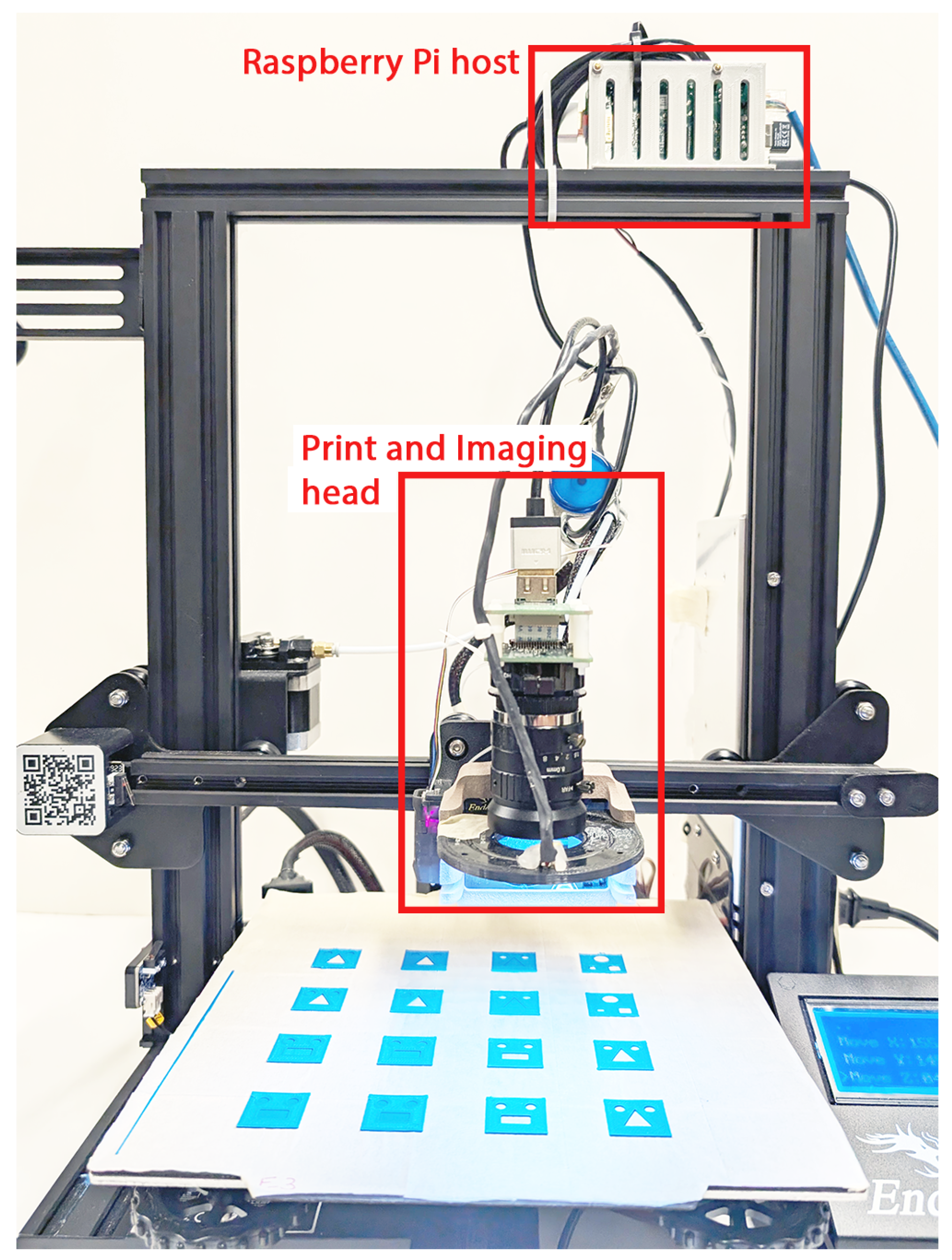A Raspberry Pi 2 Model B (Raspberry Pi Foundation, Cambridge, UK) [44] is used as the host which controls all of the functions in the AM environment. This includes reading the G-Code to control the motion of the platform and material dispensing, adjust lighting, control the image acquisition process, and perform segmentation of captured images. The experimental set-up is shown in Figure 3.

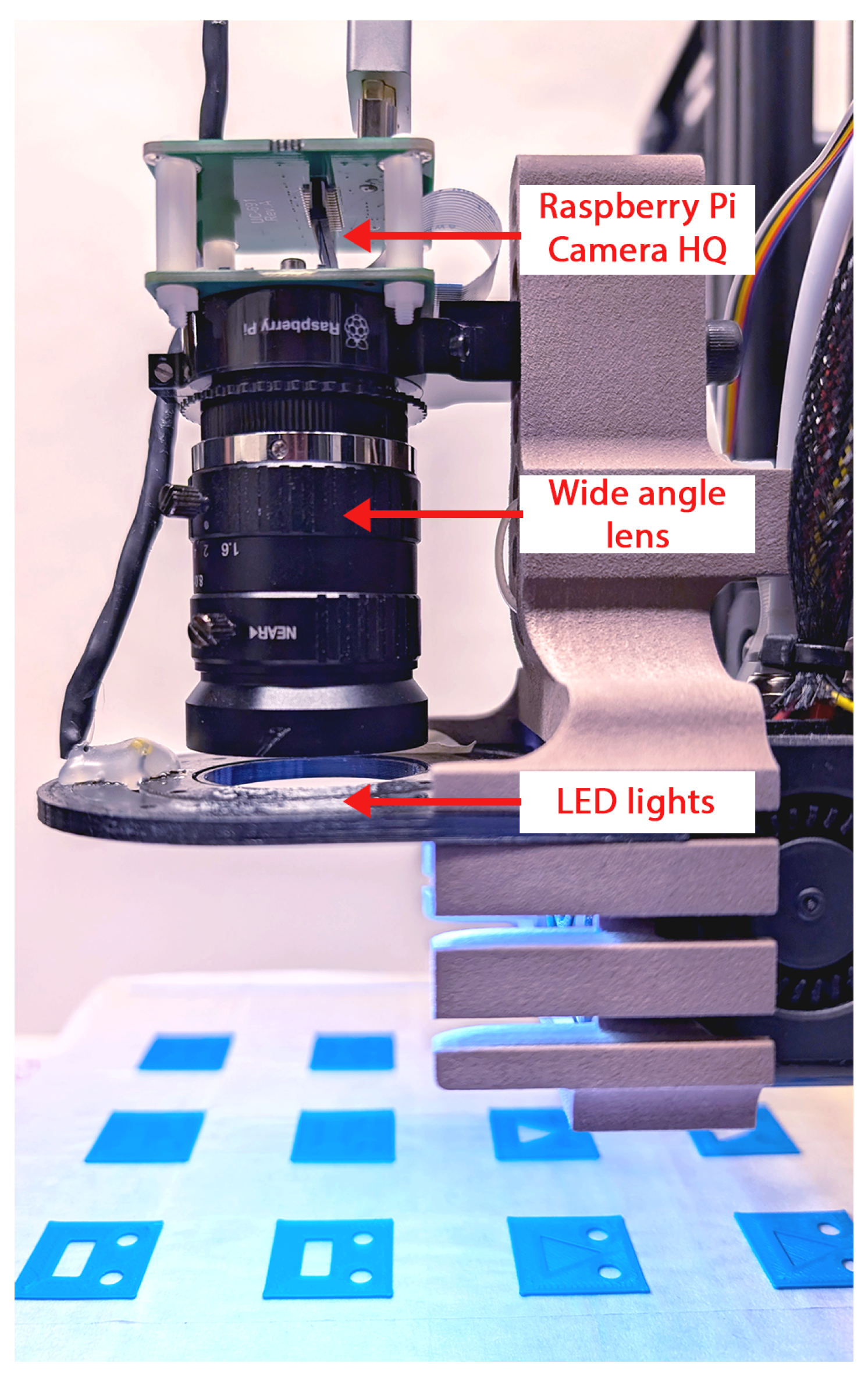
The image acquisition set-up employed a Raspberry Pi HQ camera (Raspberry Pi Foundation, Cambridge, UK) [45] which is a high-resolution image acquisition device with a Sony IMX477 backside-illuminated complementary metal-oxide semiconductor (CMOS) sensor. The image acquisition platform used an 8 mm wide-angle lens with controls for adjusting the aperture and zoom to obtain an image with the desired lighting and region of interest. The image acquisition set-up was mounted on the print head fixture of the AM platform using a custom-designed mounting bracket and provided a top view of the printed layer as shown in Figure 4.

The Raspberry Pi HQ camera could capture images at a resolution of up to $4056\times 3040$ pixels. However, a lower resolution of $1440\times 1056$ pixels was selected for the experiments, considering the feature characteristics and AM platform capabilities. This resolution corresponded to a pixel-to-millimeter scale of 28 px/mm (or 0.036 mm/px), which was sufficient to capture the features of interest on the printed part using this set-up and AM process. The minimum internal feature size which could be printed on the platform was 0.4 mm (limited by the nozzle diameter), which was more than an order of magnitude larger than the selected resolution.

The images captured by the camera were slightly distorted due to the wide-angle lens used. This distortion caused the straight edges to appear curved, as shown in Figure 5a, and would result in artificial differences between the captured image and the printed object. In order to rectify this type of image distortion, the intrinsic and extrinsic camera parameters were obtained through camera calibration using a checkerboard pattern. The intrinsic parameters provided information about the camera’s internal specifications (focal length, principal point, and distortion), which were essential for correcting distortions. The extrinsic parameters describe the camera position and orientation in space [46]. The intrinsic camera matrix was calculated by imaging a checkerboard pattern. The calibration steps were discussed in detail in our previous publication [34], and as such, they are not repeated in this article. The evaluated camera intrinsic matrix K and distortion coefficients D specific to this experimental set-up are shown in Equations (7) and (8), respectively. Using the evaluated camera calibration parameters, the obtained postprocessed image with straight lines is shown in Figure 5b:

$$K=\left[\begin{array}{ccc}4131.69& 0& 1023.20\\ 0& 4116.06& 700.98\\ 0& 0& 1\end{array}\right]$$

(7)

$$D=\left[\begin{array}{ccccc}-0.2361& -1.2055& 0.0205& 0.0002& 10.1491\end{array}\right]$$

(8)

The captured images were first processed to enhance their edge definition. Then, the color images were converted to grayscale to simplify subsequent processing steps. The image contrast was automatically adjusted using histogram equalization to improve the visibility of the external and internal edges. However, the contrast processing step also increased the image noise, which resulted in artificial textures on the part and the background becoming more prominent. In order to reduce this noise, a low-intensity Gaussian blur filter with a kernel size of $3\times 3$ was applied to the processed image. These images were then segmented using each segmentation method.

4. Results

A series of experiments was performed to evaluate the performance of each image segmentation method. A top-view image of the most recent printed part layer was captured using the developed set-up (see Section 3.5). The set-up was calibrated for lens distortion and scale accuracy to ensure that the captured images were accurate representations of the actual 3D printed parts.

A ground truth was created to evaluate the performance of each segmentation method. The processed image was converted into a binary mask using thresholding and then ‘cleaned up’ to remove any unwanted pixels. In addition to cleaning up the image, any discontinuities in the edges were corrected to ensure that the ground truth was as close to an accurate representation of the actual part as possible. The ground truth was manually prepared using Microsoft Paint v11 (an image processing application) under Microsoft Windows 11. The final preprocessed part image was analyzed by each segmentation method and compared to the ground truth to evaluate the four performance metrics.

The experiments were performed for two types of parts: one with high-contrast features and the other with low-contrast features. Each part was imaged and analyzed three times by automatically moving the camera away and then bringing it back above the part in an effort to minimize the effects of noise and lightning conditions on the captured images. The results presented are the average values for the three runs.

4.1. High Contrast Features: Single-Layer Part with Internal Features

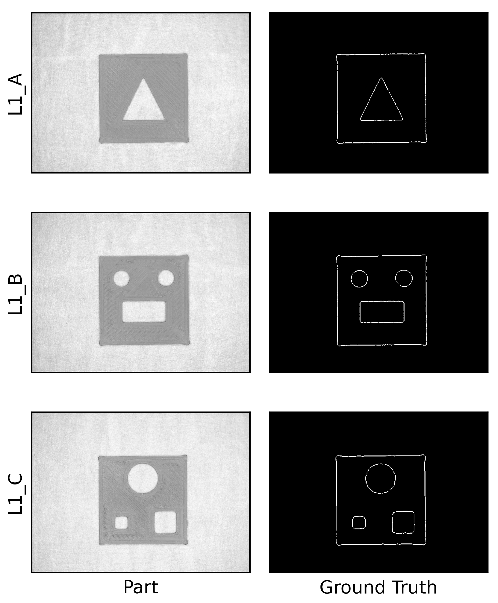
Three parts (20 mm × 20 mm) with through features were designed using Dassault Systemes SOLIDWORKS 2022 (Waltham, MA, USA) CAD software such that the bed would be visible. The through features used either individually or in combination were a triangle, a circle, and a rectangle. The three parts were labeled as L1_A, L1_B, and L1_C depending on their features, and they are shown along with their respective ground truths in Figure 6.

A single layer (thickness 0.20 mm) for each part was printed using blue poly-lactic acid (PLA) filament on a white build platform, resulting in high contrast between the part and the platform bed, since the platform bed was visible through the features and around the external edges. The processed images were analyzed using each segmentation method, with the imaging results shown in Figure 7.

In order to evaluate the performance metrics, a confusion matrix for a layer needed to be generated. This matrix included the actual (from image of the part) and predicted (from the ground truth) classes. For example, the confusion matrix (the number of pixels classified as $TP$, $FP$, $TN$, and $FN$) for one of the captured images for part L1_A using simple thresholding is shown in

Table 1. Confusion matrix for single layer part L1_A segmented using simple thresholding when compared with the ground truth.

	Predicted Positive	Predicted Negative
Actual Positive	$TP$ = 3600	$FN$ = 1852
Actual Negative	$FP$ = 427	$TN$ = 374,281

. Since the captured and ground truth images were binary with a black background and white foreground, the TN value was much higher than the other values.

Using the confusion matrix results, the performance metrics of accuracy, precision, recall, and the Jaccard index were calculated using Equations (2), (3), (4), and (6), respectively. The performance metrics (average values for three images) for each part and segmentation method are summarized in

Table 2. Performance metrics for high-contrast single layer parts with internal features.

Part	Method	Accuracy (%)	Precision (%)	Recall (%)	Jaccard Index (%)
L1_A	Simple thresholding	99.40	66.03	89.40	61.23
	Adaptive thresholding	96.53	18.92	69.11	17.44
	Sobel edge detector	75.36	3.45	85.52	3.43
	Canny edge detector	97.90	24.17	45.77	18.79
	Watershed transform	98.16	33.48	74.27	30.00
L1_B	Simple thresholding	98.80	53.47	66.96	42.31
	Adaptive thresholding	96.01	17.82	57.60	15.75
	Sobel edge detector	73.66	3.84	80.44	3.81
	Canny edge detector	97.55	24.61	43.10	18.57
	Watershed transform	97.78	31.77	62.25	26.64
L1_C	Simple thresholding	99.13	66.06	69.40	51.15
	Adaptive thresholding	95.75	14.24	44.76	12.11
	Sobel edge detector	72.55	4.01	86.95	3.98
	Canny edge detector	98.33	41.07	63.78	33.29
	Watershed transform	98.32	42.70	82.37	39.12

All results are the average values for three captured images.

.

4.2. Low-Contrast Features

The segmentation methods were also evaluated for parts exhibiting low contrast due to the previous layer(s) being visible through the features. The low-contrast features were evaluated under multiple scenarios, namely a solid first layer with the features on the second layer repeated on multiple layers and a combination of high- and low-contrast features.

4.2.1. Solid First Layer and Features on the Second Layer

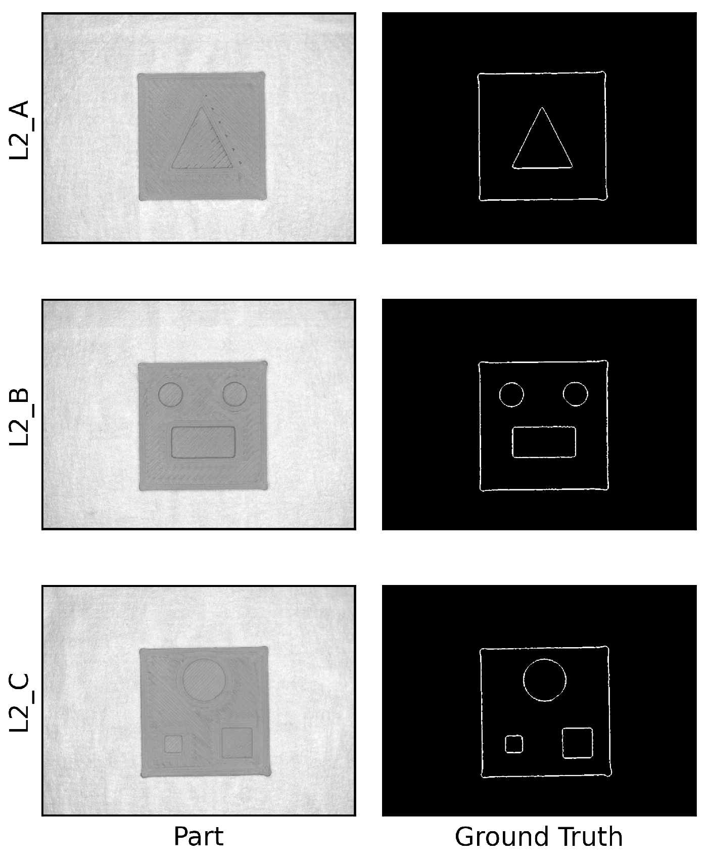
Three two-layer parts (20 mm × 20 mm) with a solid first layer and a second layer with internal features (triangle, circle, and rectangle), labeled L2_A, L2_B, and L2_C, were designed. These parts with features on the most recently printed layer were classified as low contrast due to the visibility of the previous layer through the features. 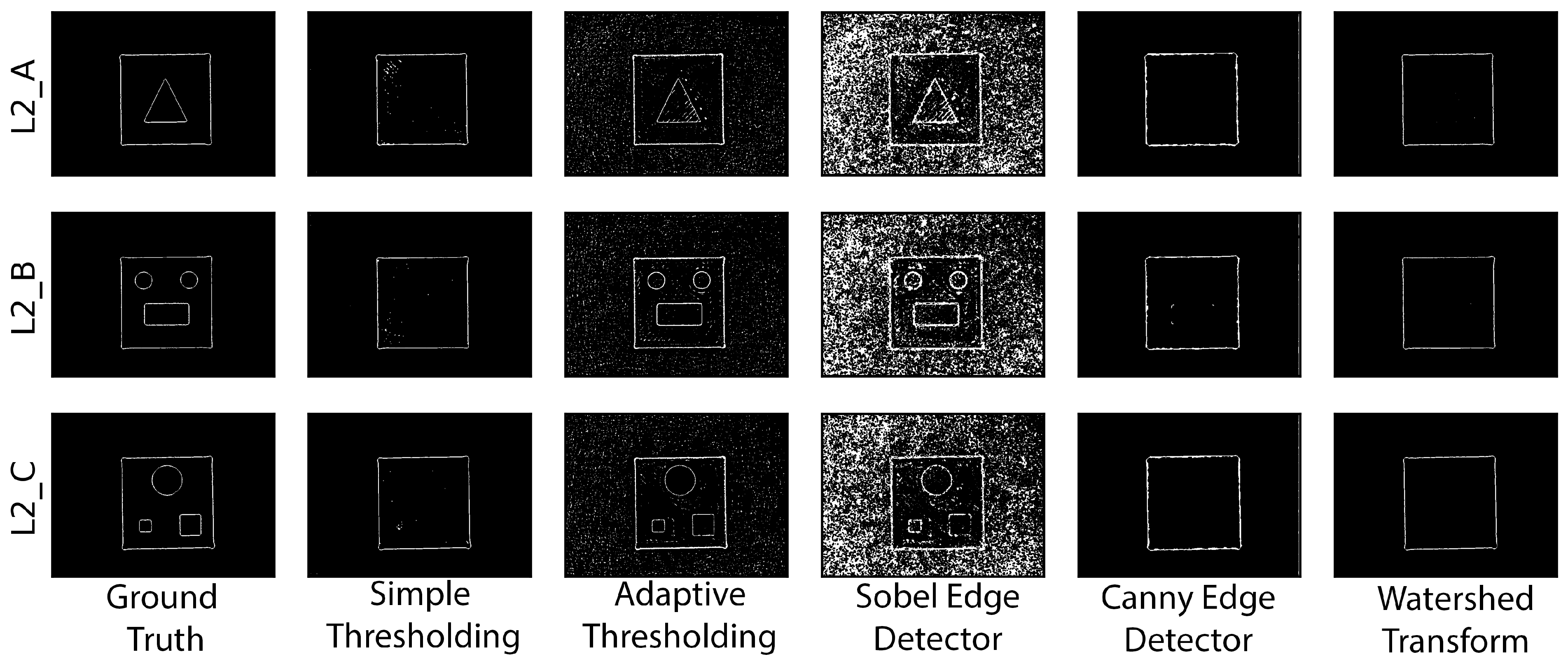The printed parts and their respective ground truths are shown in Figure 8. The printed parts were processed using each segmentation method. Representative segmented images for the second layer for each part are shown in Figure 9. The performance metrics for each segmentation method were evaluated against the ground truth for each part, and the numerical results (average values for three images) are presented in

Table 3. Performance metrics for low-contrast two-layer parts with internal features.

Part	Method	Accuracy (%)	Precision (%)	Recall (%)	Jaccard Index (%)
L2_A	Simple thresholding	99.17	60.34	69.95	47.92
	Adaptive thresholding	96.09	17.34	68.6	16.07
	Sobel edge detector	71.15	3.12	84.76	3.10
	Canny edge detector	98.04	23.85	36.15	16.78
	Watershed transform	98.08	30.50	59.80	25.31
L2_B	Simple thresholding	98.67	48.57	44.23	30.12
	Adaptive thresholding	96.34	20.73	64.58	18.62
	Sobel edge detector	74.41	4.02	81.97	3.98
	Canny edge detector	97.80	20.61	24.37	12.57
	Watershed transform	97.70	26.63	44.09	19.91
L2_C	Simple thresholding	99.13	67.09	62.54	47.86
	Adaptive thresholding	96.68	23.88	73.49	21.99
	Sobel edge detector	75.23	3.87	77.46	3.83
	Canny edge detector	97.68	19.81	27.07	12.91
	Watershed transform	97.72	26.72	45.39	20.22

All results are the average values for three captured images.

.

4.2.2. Solid First Layer and Features on Multiple Layers

The performance of the segmentation methods was also evaluated on parts with features on higher layers. Part L2_B was printed with eight layers, namely with a solid first layer and a second layer, with the internal features reproduced on all remaining layers. The segmented images are shown in Figure 10, and the numerical results (average values for three images) are presented in

Table 4. Performance metrics for a low-contrast multi-layer part (L2_B), with internal features reproduced on layers 2–8.

Part-Layer	Method	Accuracy (%)	Precision (%)	Recall (%)	Jaccard Index (%)
L2_B-L1	Simple thresholding	99.34	59.81	89.85	56.02
	Adaptive thresholding	95.06	56.42	15.49	13.83
	Sobel edge detector	82.22	85.17	6.38	6.31
	Canny edge detector	99.41	69.32	85.90	62.24
	Watershed transform	97.73	62.75	33.60	28.01
L2_B-L3	Simple thresholding	97.41	35.98	43.26	24.45
	Adaptive thresholding	94.28	45.72	19.26	15.68
	Sobel edge detector	79.16	73.80	7.82	7.61
	Canny edge detector	98.27	35.11	78.47	32.03
	Watershed transform	97.26	63.45	43.86	35.02
L2_B-L5	Simple thresholding	97.41	35.50	43.05	24.15
	Adaptive thresholding	93.01	49.74	16.59	14.21
	Sobel edge detector	76.66	72.74	6.94	6.76
	Canny edge detector	97.95	42.38	58.22	32.50
	Watershed transform	95.56	66.46	29.69	25.82
L2_B-L8	Simple thresholding	97.38	35.15	42.44	23.80
	Adaptive thresholding	93.27	53.58	18.09	15.64
	Sobel edge detector	74.95	74.63	6.63	6.48
	Canny edge detector	97.79	47.26	52.76	33.19
	Watershed transform	95.33	58.46	26.84	22.54

Note that L2_B-Lj refers to part L2_B in layer Lj, where $j(j=1,3,5,8)$. All results are the average values for three captured images.

.

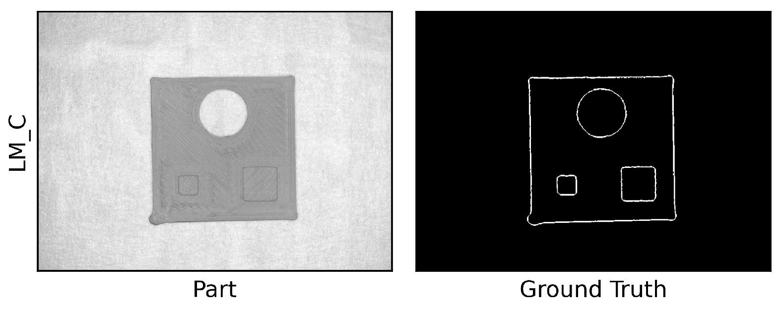
4.2.3. Combination of High- and Low-Contrast Features

An additive manufactured part may have a combination of high- and low-contrast features, where the previous layer is visible through some internal features (low contrast) while others are through-hole-type features which extend through all printed layers. The printer bed might be visible through such features (high contrast). A three-layer part, LM_C, was printed with a combination of high- and low-contrast features to evaluate whether the segmentation methods can identify features with different contrast levels on the same layer. The printed parts and their respective ground truths are shown in Figure 11. Segmented images are shown in Figure 12, and the performance metrics’ numerical results (average values for three images) are summarized in

Table 5. Performance metrics for a combination of high- and low-contrast two-layer part with internal features.

Part	Method	Accuracy (%)	Precision (%)	Recall (%)	Jaccard Index (%)
LM_C	Simple thresholding	99.14	64.81	71.45	51.48
	Adaptive thresholding	96.24	20.38	67.05	18.52
	Sobel edge detector	72.49	3.80	84.76	3.78
	Canny edge detector	97.78	25.54	38.79	18.21
	Watershed transform
	Without edge correction	98.01	34.32	61.77	28.31
	With edge correction	98.89	66.47	73.19	56.11

All results are the average values for three captured images.

.

4.2.4. Watershed Transform Observation

During the analysis of the watershed transform output, it was observed that the image boundary which was automatically added by this method was also detected as an edge with a thickness of two pixels. This artificial edge was included in the initial evaluation and negatively affected the performance metrics for this segmentation method. In order to evaluate the effect of this artificial edge on the performance metrics, the LM_C part was further processed by manually editing and removing the artificial edge using Microsoft Paint v11. Then, the performance metrics were re-evaluated using this corrected image, and the results are shown in Table 5.

5. Discussion

The results of the experiments show that the performance of the segmentation methods was highly dependent on the contrast between the layer being analyzed and the background. Additionally, any noise or texture on the part could affect the performance of the segmentation methods. The results can be further discussed while considering high- and low-contrast features. The discussion for the watershed transform was based on the images used for all segmentation methods and without any correction of the artificial edge added by the method.

5.1. High-Contrast Features

For parts with high-contrast features, multiple segmentation methods were successful in segmenting the external and internal features. Simple thresholding methods performed robustly, achieving high scores across all metrics. For example, for sample L1_A, thresholding achieved $99.40\%$ accuracy, $66.03\%$ precision, $89.40\%$ recall, and a $61.23\%$ Jaccard index. Adaptive thresholding, while segmenting the features, showed lower precision and Jaccard index scores due to its sensitivity to noise and texture variations on the evaluated layer and the bed. The Canny edge detector detected most high-contrast edges, but when compared with the thresholding method, it scored lower in all metrics, which can be attributed to the broken edges in the segmentation outputs. The Sobel edge detector had the poorest performance among the selected methods, with low scores across all metrics due to its sensitivity to texture noise on the surface of the evaluated layer and the bed. The watershed transform provided a balanced performance, segmenting strong edges with high accuracy and recall but lower precision and Jaccard index scores.

5.2. Low-Contrast Features

The performance of the segmentation methods was significantly reduced for the parts with low-contrast features. The contrast between the part and platform bed visible around the layer edge was still high, making it difficult to choose a suitable threshold value for the thresholding methods. For example, for part L2_B thresholding and Canny edge detection were both able to segment the external boundary of the part but had difficulties segmenting the internal features, as evident by the low Jaccard index scores. Adaptive thresholding and the Sobel edge detector showed poor performance across all metrics due to their sensitivity to noise and texture variations. Since adaptive thresholding relies on localized regions within an image, it often introduces noise into the segmentation output due to variations in the surface textures. This is highly relevant when processing images of FFF AM parts, as the filament strands and other weak edges are also segmented by this method.

Even though the watershed transform had poor performance for the low-contrast internal features, it was able to segment the external boundary of the part. However, the segmentation output showed significant over-segmentation due to the in-layer texture.

As more layers with the same feature(s) at the same locations were printed, the contrast between the part and the platform bed improved, making it easier for the segmentation methods to identify these features. Layer 3 (L2_B-L3) exhibited poor performance across all segmentation methods due to the low-contrast internal features. However, the performance improved as more layers were printed, such as at analyzed layers 5 and 8 for parts L2_B-L5 and L2_B-L8.

5.3. Combination of High- and Low-Contrast Features

For parts with combined high- and low-contrast features such as part LM_C, the segmentation methods faced additional challenges due to the varying contrast for different features. Simple thresholding, the Canny edge detector, and the watershed transform were only able to detect the high-contrast features. Adaptive thresholding and the Sobel edge detector were able to detect most edges, but the output was incredibly noisy, with a high number of false edges detected.

Simple thresholding showed lower precision ($64.81\%$) and recall ($71.45\%$) scores due to the need to balance between high- and low-contrast features. Although adaptive thresholding was able to segment all features, it showed decreased performance, with $96.24\%$ accuracy, $20.38\%$ precision, and $18.52\%$ for the Jaccard index, suggesting a significant number of false positives due to mixed contrast conditions. The Canny edge detector managed to adapt moderately well to the low-contrast scenarios, reflected in the $97.78\%$ accuracy, $25.54\%$ precision, and $18.21\%$ Jaccard index scores. However, this method demonstrated limitations in handling mixed contrast and noise. The Sobel edge detector, while able to detect high- and low-contrast features, continued to show overall weak performance due to high textural noise. The watershed transform showed balanced performance, with an accuracy score of $98.01\%$, but it could not capture the finer details, yielding lower precision ($34.32\%$), recall ($61.77\%$), and Jaccard index ($28.31\%$) values.

The results for both high and low contrast highlight difficulties in successfully segmenting all of the features for all of the printed parts. Most segmentation methods reliably segmented the external geometry and high-contrast internal features. However, methods such as simple thresholding, the Canny edge detector, and the watershed transform did not perform adequately with the low-contrast parts and could not reliably segment the internal features when the previous layer was visible through them. Adaptive thresholding and the Sobel edge detector were the only methods which were able to segment high- and low-contrast features. However, the segmentation outputs were heavily affected by textural and image noise.

This trend was also observed for the low-contrast parts with more than two layers. As the contrast improved at higher layers, the performance of adaptive thresholding and the Sobel edge detector also improved. However, simple thresholding, the Canny edge detector, and the watershed transform remained ineffective in segmenting low-contrast features across all layers.

6. Conclusions

Fabricating high quality parts using AM is an important research area for ensuring that manufactured parts meet defined geometric specifications and performance requirements. The layer-by-layer nature of AM introduces several challenges for in situ monitoring of internal and external features, especially when intricate geometric features, complex material compositions, and varying surface textures are involved. Accurate feature recognition at the layer level is essential to address these challenges effectively.

In this research, five image segmentation methods were evaluated for the layer-by-layer in situ analysis of parts printed using the FFF additive manufacturing process for quality control assessment. The segmentation methods evaluated were simple thresholding, adaptive thresholding, the Sobel edge detector, the Canny edge detector, and the watershed transform. The performance of these methods was assessed using the accuracy, precision, recall, and Jaccard index metrics for parts with low and high contrast and a combination thereof.

The results show that simple thresholding and the watershed transform are reliable segmentation methods and were effective for high-contrast features, with high precision and Jaccard index scores. However, as the complexity of the printed part increased, with multiple layers and varying contrast conditions, the performance of these methods declined. Adaptive thresholding and the Sobel edge detector, despite being effective in certain conditions, are sensitive to noise and texture variations, especially for low-contrast internal features. The Canny edge detector, while proficient in detecting sharp edges, faced challenges with broken and poorly shaped edges due to noise sensitivity and gradient textures.

This experimental evaluation identified that the effectiveness of a segmentation method is highly dependent on the contrast between the part and the background, as well as the noise and texture on the part surface. As such, it is important to select the appropriate segmentation method tailored to the specific characteristics of the AM process and the imaging conditions. In future work, the integration of machine learning techniques to enhance segmentation performance, particularly for low-contrast and textured parts, will be explored. The developed experimental set-up may be employed to further research the segmentation output for automatic dimensional analysis of the internal and external features and overall geometry in situ.

References

- Mireles, J.; Ridwan, S.; Morton, P.A.; Hinojos, A.; Wicker, R.B. Analysis and correction of defects within parts fabricated using powder bed fusion technology. Surf. Topogr. Metrol. Prop. 2015, 3, 034002. [Google Scholar] [CrossRef]
- Du Plessis, A.; Le Roux, S.G.; Els, J.; Booysen, G.; Blaine, D.C. Application of microCT to the non-destructive testing of an additive manufactured titanium component. Case Stud. Nondestruct. Test. Eval. 2015, 4, 1–7. [Google Scholar] [CrossRef]
- Du Plessis, A.; Le Roux, S.G.; Booysen, G.; Els, J. Quality Control of a Laser Additive Manufactured Medical Implant by X-Ray Tomography. 3D Print. Addit. Manuf. 2016, 3, 175–182. [Google Scholar] [CrossRef]
- Rieder, H.; Dillhöfer, A.; Spies, M.; Bamberg, J.; Hess, T. Online Monitoring of Additive Manufacturing Processes Using Ultrasound. 2016. Available online: https://api.semanticscholar.org/CorpusID:26787041 (accessed on 11 February 2024).
- Cerniglia, D.; Scafidi, M.; Pantano, A.; Lopatka, R. Laser ultrasonic technique for laser powder deposition inspection. Laser 2013, 6, 13. [Google Scholar]
- Petruse, R.E.; Simion, C.; Bondrea, I. Geometrical and Dimensional Deviations of Fused Deposition Modelling (FDM) Additive-Manufactured Parts. Metrology 2024, 4, 417–429. [Google Scholar] [CrossRef]
- Straub, J. Initial work on the characterization of additive manufacturing (3D printing) using software image analysis. Machines 2015, 3, 55–71. [Google Scholar] [CrossRef]
- Liu, C.; Law, A.C.C.; Roberson, D.; Kong, Z.J. Image analysis-based closed loop quality control for additive manufacturing with fused filament fabrication. J. Manuf. Syst. 2019, 51, 75–86. [Google Scholar] [CrossRef]
- Nuchitprasitchai, S.; Roggemann, M.; Pearce, J.M. Factors effecting real-time optical monitoring of fused filament 3D printing. Prog. Addit. Manuf. 2017, 2, 133–149. [Google Scholar] [CrossRef]
- Rossi, A.; Moretti, M.; Senin, N. Layer inspection via digital imaging and machine learning for in-process monitoring of fused filament fabrication. J. Manuf. Process. 2021, 70, 438–451. [Google Scholar] [CrossRef]
- Moretti, M.; Rossi, A.; Senin, N. In-process monitoring of part geometry in fused filament fabrication using computer vision and digital twins. Addit. Manuf. 2021, 37, 101609. [Google Scholar] [CrossRef]
- Garanger, K.; Khamvilai, T.; Feron, E. 3D Printing of a Leaf Spring: A Demonstration of Closed-Loop Control in Additive Manufacturing. In Proceedings of the 2018 IEEE Conference on Control Technology and Applications (CCTA), Copenhagen, Denmark, 21–24 August 2018; pp. 465–470. [Google Scholar] [CrossRef]
- Cummings, I.T.; Bax, M.E.; Fuller, I.J.; Wachtor, A.J.; Bernardin, J.D. A Framework for Additive Manufacturing Process Monitoring & Control. In Topics in Modal Analysis & Testing, Volume 10; Mains, M., Blough, J., Eds.; Series Title: Conference Proceedings of the Society for Experimental Mechanics Series; Springer International Publishing: Cham, Switzerland, 2017; pp. 137–146. [Google Scholar] [CrossRef]
- Gaikwad, A.; Yavari, R.; Montazeri, M.; Cole, K.; Bian, L.; Rao, P. Toward the digital twin of additive manufacturing: Integrating thermal simulations, sensing, and analytics to detect process faults. IISE Trans. 2020, 52, 1204–1217. [Google Scholar] [CrossRef]
- Knapp, G.L.; Mukherjee, T.; Zuback, J.S.; Wei, H.L.; Palmer, T.A.; De, A.; DebRoy, T. Building blocks for a digital twin of additive manufacturing. Acta Mater. 2017, 135, 390–399. [Google Scholar] [CrossRef]
- Nath, P.; Mahadevan, S. Probabilistic Digital Twin for Additive Manufacturing Process Design and Control. J. Mech. Des. 2022, 144, 091704. [Google Scholar] [CrossRef]
- Baumann, F.; Roller, D. Vision based error detection for 3D printing processes. MATEC Web Conf. 2016, 59, 06003. [Google Scholar] [CrossRef]
- Lyngby, R.A.; Wilm, J.; Eiríksson, E.R.; Nielsen, J.B.; Jensen, J.N.; Aanæs, H.; Pedersen, D.B. In-line 3D print failure detection using computer vision. In Proceedings of the Dimensional Accuracy and Surface Finish in Additive Manufacturing, Leuven, Belgium, 10–12 October 2017; Available online: https://api.semanticscholar.org/CorpusID:115671036 (accessed on 30 April 2024).
- Jin, Z.; Zhang, Z.; Gu, G.X. Autonomous in-situ correction of fused deposition modeling printers using computer vision and deep learning. Manuf. Lett. 2019, 22, 11–15. [Google Scholar] [CrossRef]
- Shen, H.; Sun, W.; Fu, J. Multi-view online vision detection based on robot fused deposit modeling 3D printing technology. Rapid Prototyp. J. 2019, 25, 343–355. [Google Scholar] [CrossRef]
- Jin, Z.; Zhang, Z.; Gu, G.X. Automated Real-Time Detection and Prediction of Interlayer Imperfections in Additive Manufacturing Processes Using Artificial Intelligence. Adv. Intell. Syst. 2020, 2, 1900130. [Google Scholar] [CrossRef]
- Farhan Khan, M.; Alam, A.; Ateeb Siddiqui, M.; Saad Alam, M.; Rafat, Y.; Salik, N.; Al-Saidan, I. Real-time defect detection in 3D printing using machine learning. Mater. Today: Proc. 2021, 42, 521–528. [Google Scholar] [CrossRef]
- He, K.; Zhang, Q.; Hong, Y. Profile monitoring based quality control method for fused deposition modeling process. J. Intell. Manuf. 2019, 30, 947–958. [Google Scholar] [CrossRef]
- Yi, W.; Ketai, H.; Xiaomin, Z.; Wenying, D. Machine vision based statistical process control in fused deposition modeling. In Proceedings of the 2017 12th IEEE Conference on Industrial Electronics and Applications (ICIEA), Siem Reap, Cambodia, 18–20 June 2017; pp. 936–941. [Google Scholar] [CrossRef]
- Delli, U.; Chang, S. Automated Process Monitoring in 3D Printing Using Supervised Machine Learning; Elsevier B.V.: Amsterdam, The Netherlands, 2018; Volume 26, pp. 865–870. ISSN 23519789. [Google Scholar] [CrossRef]
- Nuchitprasitchai, S.; Roggemann, M.; Pearce, J. Three Hundred and Sixty Degree Real-Time Monitoring of 3-D Printing Using Computer Analysis of Two Camera Views. J. Manuf. Mater. Process. 2017, 1, 2. [Google Scholar] [CrossRef]
- Holzmond, O.; Li, X. In situ real time defect detection of 3D printed parts. Addit. Manuf. 2017, 17, 135–142. [Google Scholar] [CrossRef]
- Lyu, J.; Manoochehri, S. Online Convolutional Neural Network-based anomaly detection and quality control for Fused Filament Fabrication process. Virtual Phys. Prototyp. 2021, 16, 160–177. [Google Scholar] [CrossRef]
- Grand-Brochier, M.; Vacavant, A.; Cerutti, G.; Bianchi, K.; Tougne, L. Comparative study of segmentation methods for tree leaves extraction. In Proceedings of the International Workshop on Video and Image Ground Truth in Computer Vision Applications, St. Petersburg, Russia, 15 July 2013; pp. 1–7. [Google Scholar] [CrossRef]
- Marcomini, L.A.; Cunha, A.L. A Comparison between Background Modelling Methods for Vehicle Segmentation in Highway Traffic Videos. arXiv 2018. [Google Scholar] [CrossRef]
- Ng, H.; Ong, S.; Foong, K.; Goh, P.; Nowinski, W. Medical Image Segmentation Using K-Means Clustering and Improved Watershed Algorithm. In Proceedings of the 2006 IEEE Southwest Symposium on Image Analysis and Interpretation, Denver, CO, USA, 26–28 March 2006; pp. 61–65. [Google Scholar] [CrossRef]
- Huang, Y.L.; Chen, D.R. Watershed segmentation for breast tumor in 2-D sonography. Ultrasound Med. Biol. 2004, 30, 625–632. [Google Scholar] [CrossRef]
- A S, R.A.; Gopalan, S. Comparative Analysis of Eight Direction Sobel Edge Detection Algorithm for Brain Tumor MRI Images. Procedia Comput. Sci. 2022, 201, 487–494. [Google Scholar] [CrossRef]
- Saini, T.; Shiakolas, P.S. A Framework for In-Situ Vision Based Detection of Part Features and its Single Layer Verification for Additive Manufacturing. In Proceedings of the ASME International Mechanical Engineering Congress and Exposition, Volume 3: Advanced Manufacturing, New Orleans, LA, USA, 29 October–2 November 2023; p. V003T03A083. [Google Scholar] [CrossRef]
- OpenCV. OpenCV 4.6.0. 2023. Available online: https://docs.opencv.org/4.6.0 (accessed on 1 May 2024).
- OpenCV. OpenCV: Basic Thresholding Operations. 2023. Available online: https://docs.opencv.org/4.x/db/d8e/tutorial_threshold.html (accessed on 1 May 2024).
- OpenCV. OpenCV: Image Thresholding. 2023. Available online: https://docs.opencv.org/3.4/d7/d4d/tutorial_py_thresholding.html (accessed on 1 May 2024).
- OpenCV. Adaptative Thresholding. 2024. Available online: https://docs.opencv.org/4.x/d7/d4d/tutorial_py_thresholding.html#autotoc_md1459 (accessed on 1 May 2024).
- Sobel, I.; Feldman, G.M. An Isotropic 3×3 Image Gradient Operator. 1990. Available online: https://api.semanticscholar.org/CorpusID:59909525 (accessed on 1 May 2024).
- Canny, J. A Computational Approach to Edge Detection. IEEE Trans. Pattern Anal. Mach. Intell. 1986, PAMI-8, 679–698. [Google Scholar] [CrossRef]
- OpenCV. OpenCV: Canny Edge Detector. 2023. Available online: https://docs.opencv.org/3.4/da/d5c/tutorial_canny_detector.html (accessed on 13 May 2024).
- Digabel, H.; Lantuéjoul, C. Iterative algorithms. In Proceedings of the 2nd European Symposium Quantitative Analysis of Microstructures in Material Science, Biology and Medicine; Riederer Verlag: Munich, Germany, 1978; Volume 19, p. 8. [Google Scholar]
- Shenzhen Creality 3D Technology Co. Creality Ender 3 Pro. 2023. Available online: https://www.creality.com/products/ender-3-pro-3d-printer (accessed on 12 December 2023).
- Raspberry Pi Foundation. Raspberry Pi 2 Model B. 2023. Available online: https://www.raspberrypi.com/products/raspberry-pi-2-model-b/ (accessed on 12 December 2023).
- Raspberry Pi Foundation. Raspberry Pi HQ Camera. 2023. Available online: https://www.raspberrypi.com/products/raspberry-pi-high-quality-camera/ (accessed on 12 December 2023).
- Hartley, R.; Zisserman, A. Camera Models. In Multiple View Geometry in Computer Vision; Cambridge University Press: Cambridge, UK, 2004; pp. 153–177. [Google Scholar] [CrossRef]
Figure 1.
Proposed in situ layer inspection process flow for AM independent of segmentation approach employed.
Figure 2.
Flow of information between the various components of the experimental set-up.
Figure 3.
Custom developed experimental set-up controlled by a Raspberry Pi.
Figure 4.
Close-up of the print and imaging head, showing the Raspberry Pi HQ camera, lens, and LED lights.
Figure 5.
Camera calibration. (a) Raw image before camera calibration with distorted straight edges. (b) Image after camera calibration with undistorted straight edges.
Figure 6.
Single layer parts with high-contrast features: printed and ground truth.
Figure 7.
Segmented images for single layer parts with internal features.
Figure 8.
Two-layer parts with low-contrast features on second layer: printed and ground truth.
Figure 9.
Segmented images for a solid first layer and features on the second layer.
Figure 10.
Segmented images for solid first layer with features reproduced on subsequent layers.
Figure 11.
Three-layer part with a combination of high- and low-contrast features, showing printed and ground truth for the topmost layer.
Figure 12.
Segmented images for combined high- and low-contrast features.