Various Grids in Moiré Measurements

Abstract

The moiré effect is typically observed in regular periodic structures and sometimes in random (aperiodic) structures. However, currently, only regular graphical objects are used in measurements. We propose using graphical objects that are not regular but not entirely random and that resemble rows, such as grids of dotted lines or matrixes of dots. The moiré effect in such objects may become similar to the moiré effect in regular graphical objects if a relatively simple modification of the image processing algorithm is applied. We demonstrated that the results of measurements with five different graphical objects arranged in rows (including text) are similar. Using such objects can be helpful for practical moiré measurements.

1. Introduction

Moiré is an effect that forms patterns with a longer spatial period due to the interference of similar periodic structures with shorter periods [1,2,3,4]. Sciammarella [3] states that a “superposition of the two gratings produces the moiré patterns”. Amidror [1] says that the moiré is “a new pattern of alternating dark and bright areas which is observed at the superposition, although it does not appear in any of the original structures”. Bryngdahl [2] refers to them as “low-frequency moiré patterns” “caused by superposing two similar grid structures”. Oster et al. [4] note that “a moiré pattern may be described as a locus of points of intersection of two overlapping figures”. All these citations characterize the moiré pattern as a low-frequency component of an overlap (superposition, superimposition, interaction) of grids (gratings), at least one of which (close to the observer/photo camera) is transparent. The superposition is mathematically expressed as the multiplication. The low-frequency components can be obtained by averaging, filtration, and the like.

The formal definition of the moiré effect is as follows: “The moiré effect is the effect of the formation of measurable patterns of a longer period caused by a point-by-point interaction in corresponding points between similar periodic structures of shorter periods and the averaging in the neighbourhood of those points” [5].

We consider the optical moiré effect in transmitted and reflected light, although the moiré patterns have been observed not only in visible light but also in infrared light [6,7], X-rays [8,9], electron beams [10,11], and even in waves on the water [12,13].

Mostly, the effect is considered in coplanar layers [1,2,14,15,16,17]. In particular, Amidror [1] and Bryngdahl [2] implicitly consider the moiré patterns in grids lying in the same plane, and the papers [14,15,16,17] investigated planar two-dimensional (2D) nano-materials, an advanced subject of contemporary physics. In these cases, everything happens in two dimensions (i.e., within a plane). The moiré effect is sometimes studied in 3D [5,18,19,20]. Namely, the paper [18] considers the moiré effect in parallel/crossing planes and circular objects like cylinders, Kafri and Glatt [19] consider the spatial (i.e., 3D) shapes of measured objects, and Weissman [20] considers the visual 3D effect in various types of displays.

Most research papers study the moiré effect in regular (repeated) graphical structures (objects). However, some authors consider the moiré effect in approximate [21] or random graphical objects [22,23]. Approximate graphical objects were intentionally or occasionally averaged to observe the moiré effect, as Glass patterns appeared because of the rotational autocorrelation of the irregular (random) dot matrix. Approximate grids [21] are averaged due to their motion. Thus, the moiré effect in irregular/aperiodic structures requires an “additional” averaging/integration.

In particular, the improved shadow moiré method in [6] is intended for IR shape measurement in subcutaneous tissue (under the skin), including a pulse measurement method. The beam alignment in invisible light [7] is based on the moiré effect. The paper [8] presents the first part of an in-depth study on moiré patterns in X-rays; the study was continued in the next issues of Acta Crystallographica in 2019 and 2020, including the theory, experiments, and computer simulations. In [9], the moiré effect is considered in application to phase contrast imaging and X-ray interferometry. Grain boundaries in graphene bilayers were identified in [10] using the moiré effect. The paper [11] discusses rotational and translational moiré patterns and how they can appear in TEM, with many examples in different materials. In [12], the moiré patterns of sound in shallow water at distances of several kilometers are considered, although they are called interference. The authors of [13] used the moiré sampling method to measure the waves on the water surface.

The moiré patterns in twisted 2D materials and their simulation are presented in [14] along with explanations of their physical nature. In [15], the moiré effect in graphene on metal substrate is investigated using a theory based on 2D Fourier transform, including rotation and scaling. In [16], the authors consider the moiré effect in twisted bilayer graphene on the so-called magic angle and apply it to reduce a local disorder. “The observation of moiré patterns in mechanically stacked graphene layers has triggered rapid progress in graphene research”, as quoted in [17], where the authors study the electronic structure, fabrication, and angle-dependent properties of this material.

Some regular grids can be represented as combinations of line gratings, and the hexagonal grid can be considered as a combination of zigzag and dashed gratings [21]. The equivalence of the magnification factor and twist angle, as well as the condition of the constant phase, were discovered in [ibid.]. The profile of the averaged grating has one maximum per period [ibid.]. The static directions can be found using periodic structures in vertical sections of the grid sinograms (i.e., their Radon transform) [ibid.].

In the 1960s, Glass [22] discovered the moiré patterns in aperiodic or random structures, named after him. Amidror [23] considers “phenomena which occur in the superposition of correlated aperiodic layers” and provides “a full general purpose and application-independent exposition of the subject” (quotations in [23]).

As soon as the moiré is an integral effect (and can be expressed as a convolution integral [1]), the grids do not necessarily consist of only solid straight lines. They need to maintain some periodicity “on average”. Thus, similar to approximate gratings [21], the lines of graphical objects can be dotted, zigzagged, or curved as long as the “traces” of some lines are preserved; that is, such almost periodic graphical objects should be “arranged in parallel rows”. We excluded the influence of a particular irregular structure by averaging the profiles.

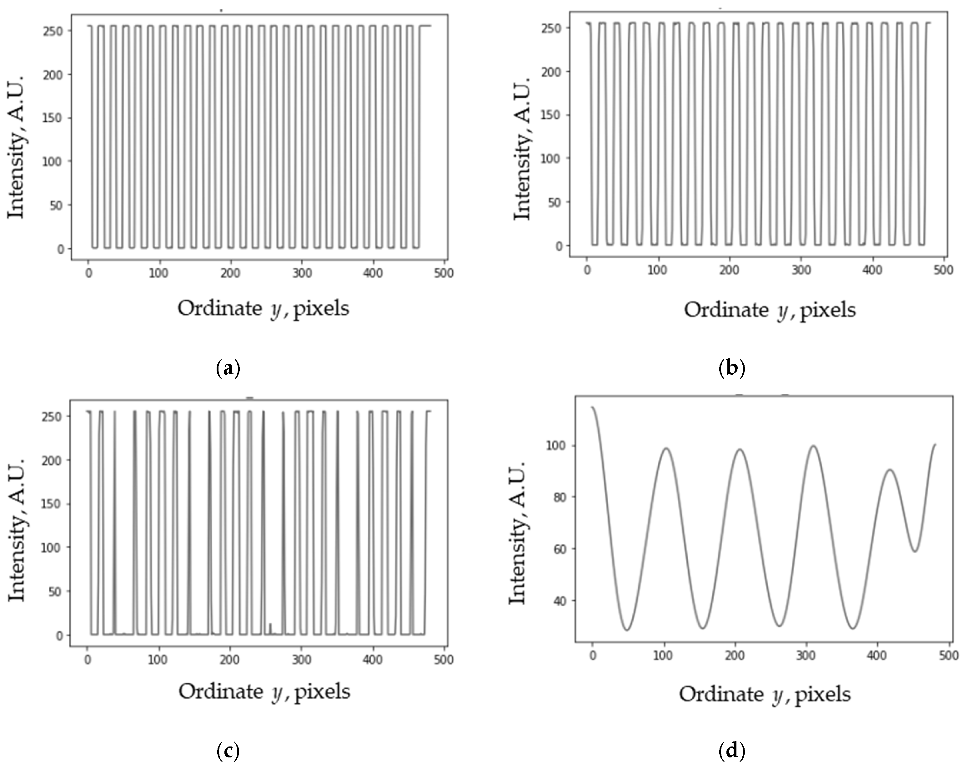
Analytically, the moiré patterns can be expressed as the filtered product of the transparency/transmittance functions of grids [18] obtained after a low-pass filter. This is a consequence of the convolution property, sometimes expressed as follows: “Multiplication in the time domain is equivalent to the convolution in the frequency domain”. We illustrate the multiplication followed by a filtration in Figure 1.

The periods of grids in Figure 1a,b are equal to 100 and 120 arbitrary units (namely, pixels), respectively, and differ by 20%. The period of the moiré patterns in Figure 1d is 105.3 units.

As one grid is displaced (shifted), the moiré patterns are proportionally displaced. The proportionality of the phase [1] is the key to knowing the position of the grid (in the direction perpendicular to its lines) through the measurement of the displacement of the moiré patterns.

A practical application of the moiré effect is the measurement of the displacement of distant objects by optical methods [24,25,26,27,28]. Moiré measurements are usually relative; i.e., the object’s position is measured relative to a specific reference point or line. Particularly, Patorski and Kujawinska [24] present the fundamentals of moiré measurements, Post and Han [25] consider an increased sensitivity, Creath and Wyant [26] demonstrate projection methods, Khan and Wang [27] consider applications, and Walker [28] provides an overview of moiré measurements. Measuring displacements with a digital camera using the moiré effect has advantages over direct (other than moiré) measurements, not least because of the moiré magnification [29,30]. There must be two grids in moiré measurements: a grid on a measured object and a static reference grid.

Previously, we described a deferred moiré method for measuring displacements using a digital camera and regular line grids [31]. This method is based on moiré magnification [29] and phase proportionality [1]. The magnification means improved sensitivity, and the phase of the patterns means displacement. In our method, the second (reference) grid is generated by a computer. Calibration is not needed because the size of the grid attached to the object is known.

Recently, our approach was changed, and currently, we propose using irregular graphical objects that are not entirely random and that resemble rows, such as a grid of dotted lines, a matrix of dots, or a text. The current manuscript describes this approach and illustrates its flexibility with numerous examples of such objects.

Section 2 describes the measurement method, including the principles, unwrapping, approach to various graphical objects arranged in rows, alignment, and measurement system. Section 3 introduces approximate grids and similar graphical objects, shows computer simulations of the moiré effect in such grids, demonstrates measurements using several graphical objects of different types, and shows the results and analysis. Section 4 and Section 5 contain the discussion and conclusion.

2. Materials and Methods

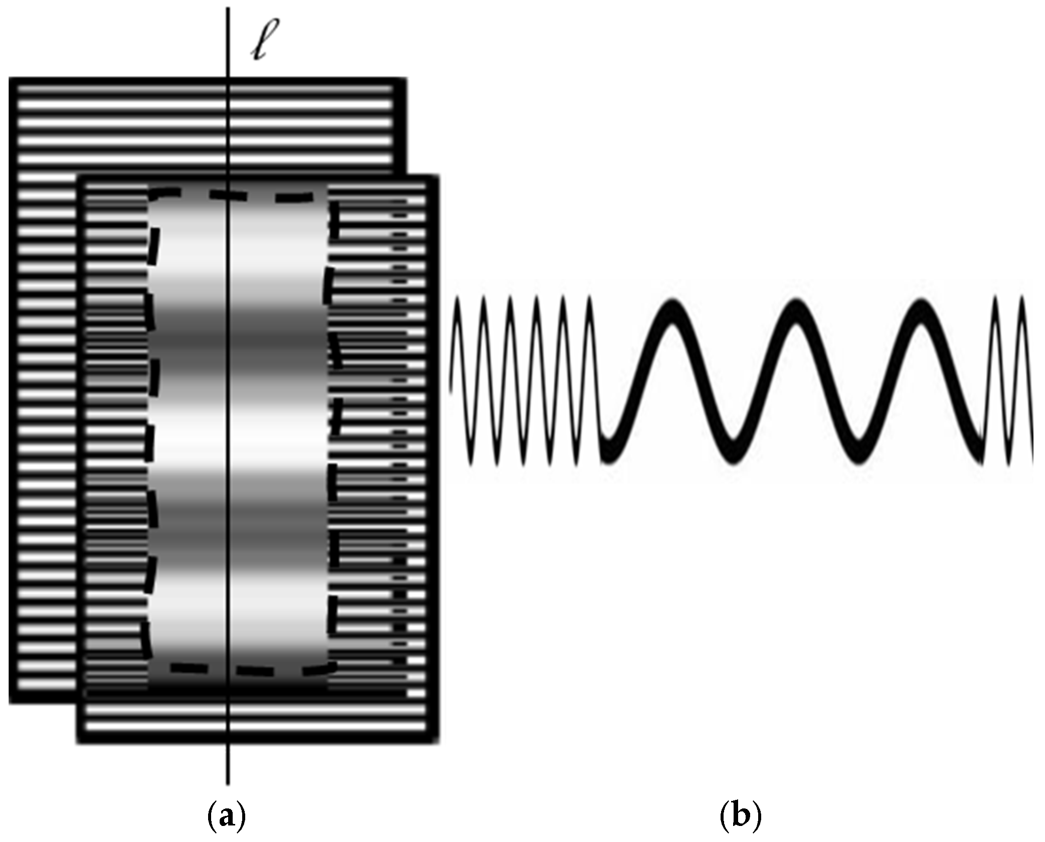
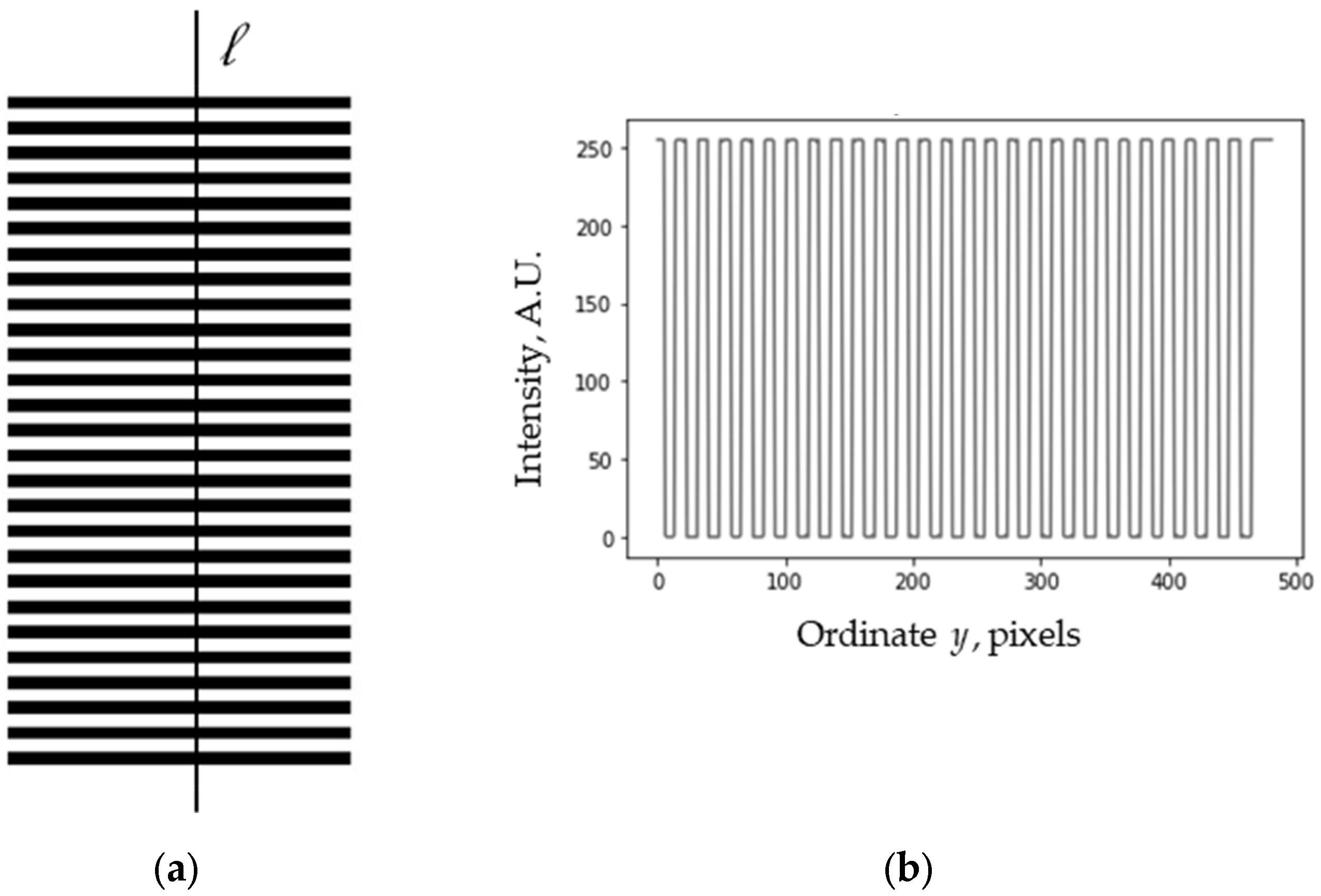
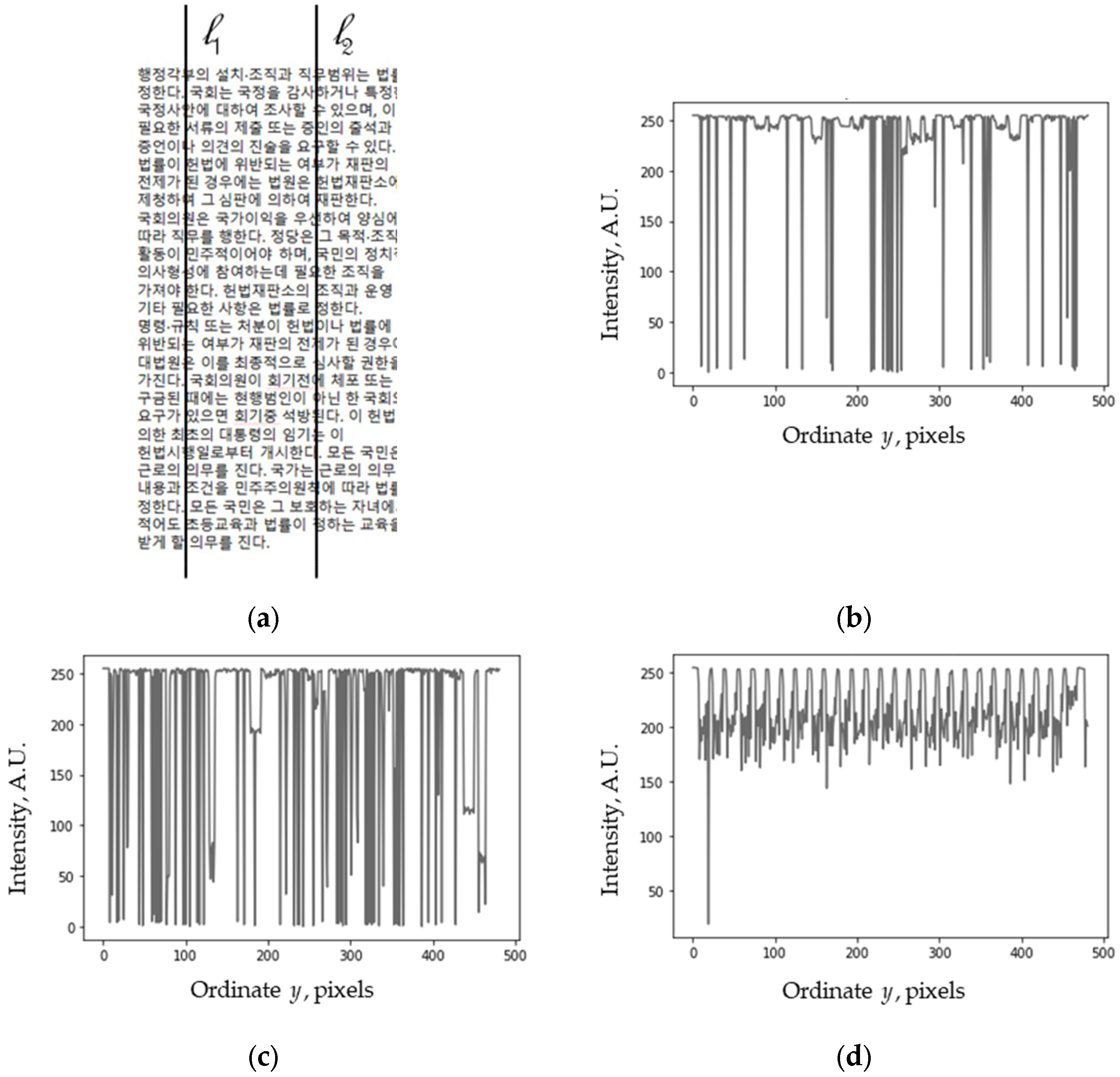
The moiré patterns appear in the region wherein two grids with parallel lines overlap (superimpose) each other (one grid is transparent). To show the pure moiré patterns themselves (which are a low-frequency component of the overlap), a low-pass filter (in the simplest case, averaging) is applied. The dashed line at the center of Figure 2a shows the result: the pure patterns. The moiré patterns in the grids with parallel lines are parallel to the grid lines. Considering the vertical cross section is sufficient to estimate the moiré patterns in parallel grids with the horizontal lines. The cross section (intensity profile) along the vertical line (l), which is perpendicular to the vertical lines of the grid, is shown in Figure 2b. Such a one-dimensional (1D) profile completely describes the moiré effect in grids with parallel lines. Therefore, we effectively consider a 1D effect.

2.1. Principle of Measurements

According to [1], the spatial period of the moiré patterns (T_M) in parallel coplanar grids of different periods is as follows:

$$T_M={\displaystyle \frac{T_1{T}_2}{\left|T_1-T_2\right|}}=T_1{\displaystyle \frac{1}{\left|\frac{T_1}{T_2}-1\right|}}$$

(1)

where T₁ and T₂ are the spatial periods of the grids.

The moiré magnification coefficient (μ) is defined as a ratio of periods:

$$\mu ={\displaystyle \frac{T_M}{T_1}}$$

(2)

The period of a grid (T) is equal to the size of the grid (L) divided by the number of intervals between the grid lines (N):

$$T={\displaystyle \frac{L}{N}}$$

(3)

Then, Equation (1) can be rewritten as follows:

$$\mu ={\displaystyle \frac{N_1}{\left|N_2-N_1\right|}}$$

(4)

Equation (4) shows that the moiré magnification coefficient is equal to the number of intervals in one grid divided by the difference between the numbers of intervals in both grids. This means that the larger of the two numbers, N₁ or N₂, determines the maximum moiré magnification under the given conditions. As a result, the more lines in the grid, the greater the moiré magnification becomes.

2.2. Unwrapping

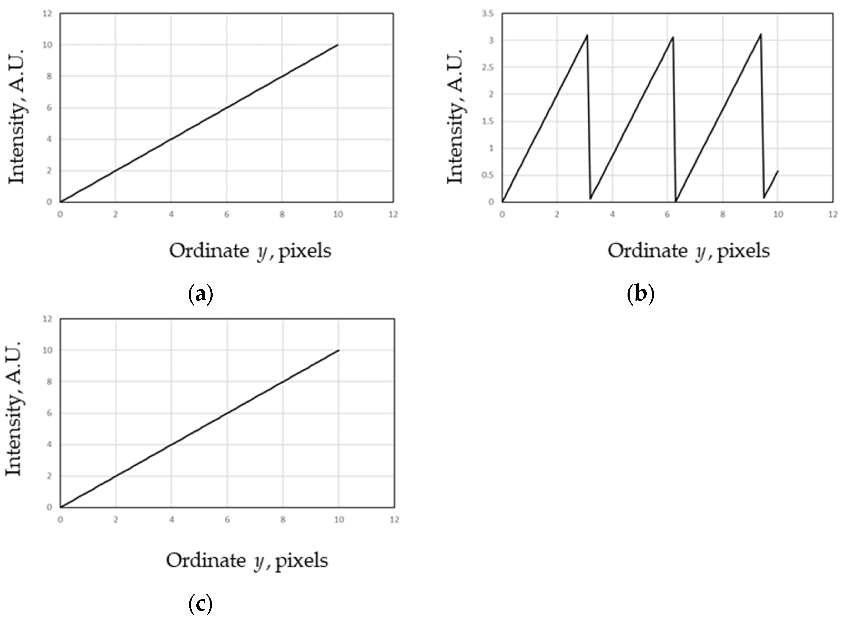
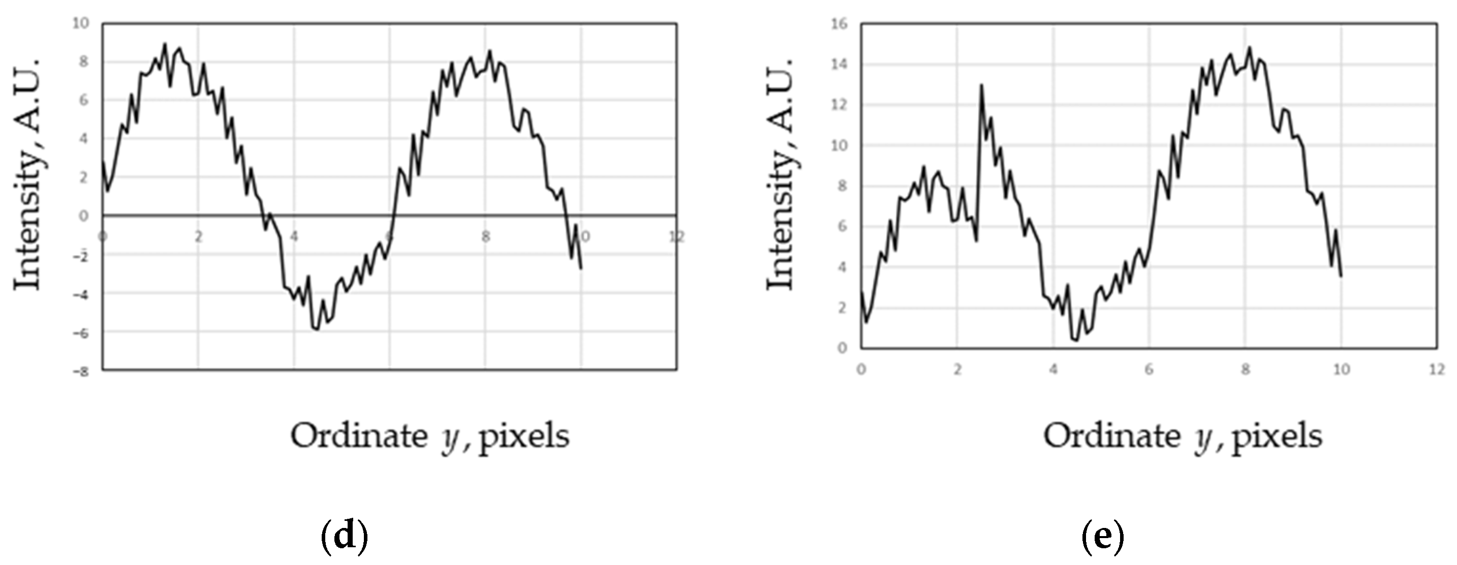
The measured phase is always within the interval [−π/2, π/2], as the principal value of multi-valued trigonometric functions (arcsine, arctangent). This effect is called folding or wrapping. Wrapping is a form of ambiguity and looks like a folded paper fan or an accordion’s expanding/contracting bellows.

Graphically, it can be imagined as measuring a wheel’s rotation angle, always within 2π, with no relation to the number of complete turns the wheel made before. As a result, when the wheel completes the full turn, the measured phase makes a “jump”. However, practically, the wheel does not make jumps in rotation; its rotation is smooth and uniform, as expected of the measured “unwrapped” phase.

Similarly, the resulting measured phase should be definite and continuous. Therefore, unwrapping (unfolding) is necessary for practical measurements, but the principal value alone is insufficient. Thus, to make the result of measurements unambiguous, we have to use some extra (additional) information, for example, the presence or absence of sharp jumps in the output signal (presumably, at the moment of wrapping). This can be solved by applying phase unwrapping methods [32,33]. An illustration of this process is shown in Figure 3 for two cases: an ideal function and a function with noise.

In the ideal case, the function is always unwrapped correctly based on the detected jumps (Figure 3c). However, in the presence of noise (practically unavoidable in real life), the results of the unwrapping may appear distorted; e.g., the output may contain an undeleted or fake jump, as in Figure 3e at x = 2.5.

2.3. Grids Other than Regular

In the described method, measurements are taken using a cross section (profile) of the image along a certain line (i.e., a 1D object). Let it be a vertical line. Measurements along all parallel lines of the same length (within the image of a regular line grid) give the same result. However, the grid is a flat 2D graphical object. This discrepancy in dimensions raises the following question: what kind of grid can be used for measurements?

From this point of view, it is useful to remember that the moiré effect was observed not only in regular graphical objects but also in aperiodic and even random structures [22,23]. In addition, approximate grids are needed for static moiré patterns in moving grids [21]. In this study, some irregular grids were found that can be used in moiré measurements.

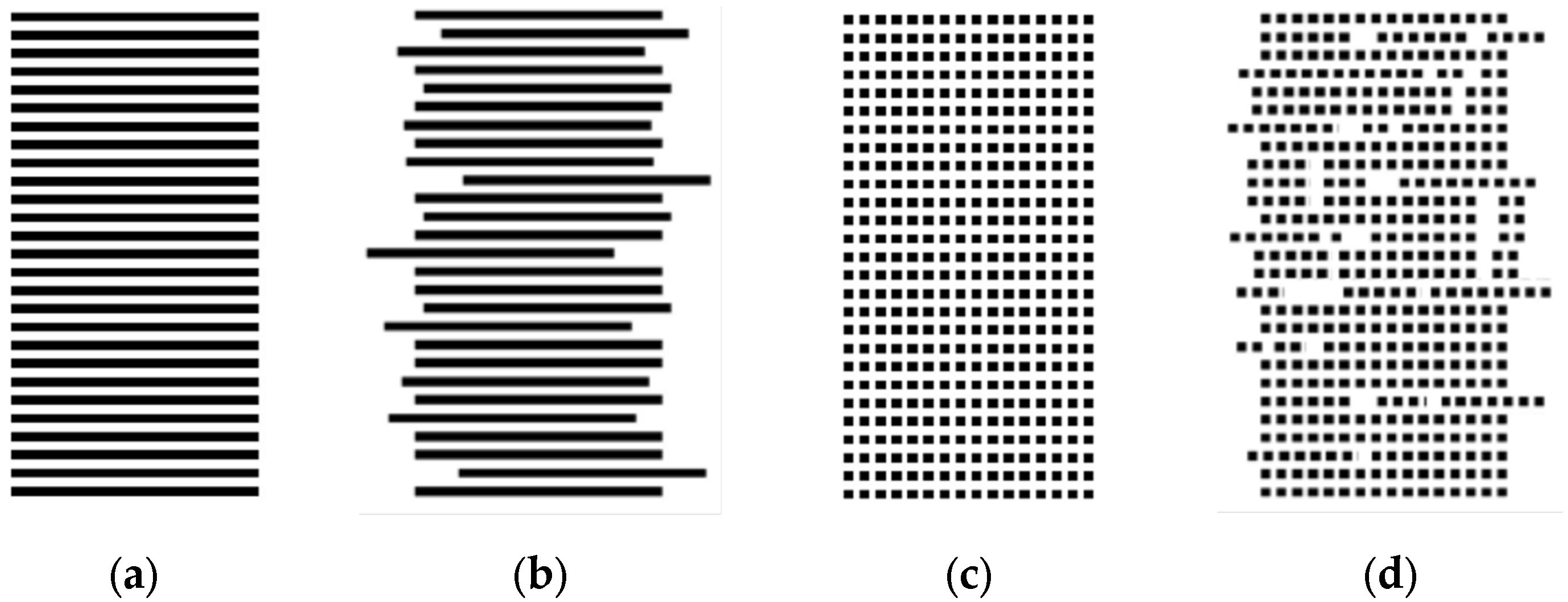
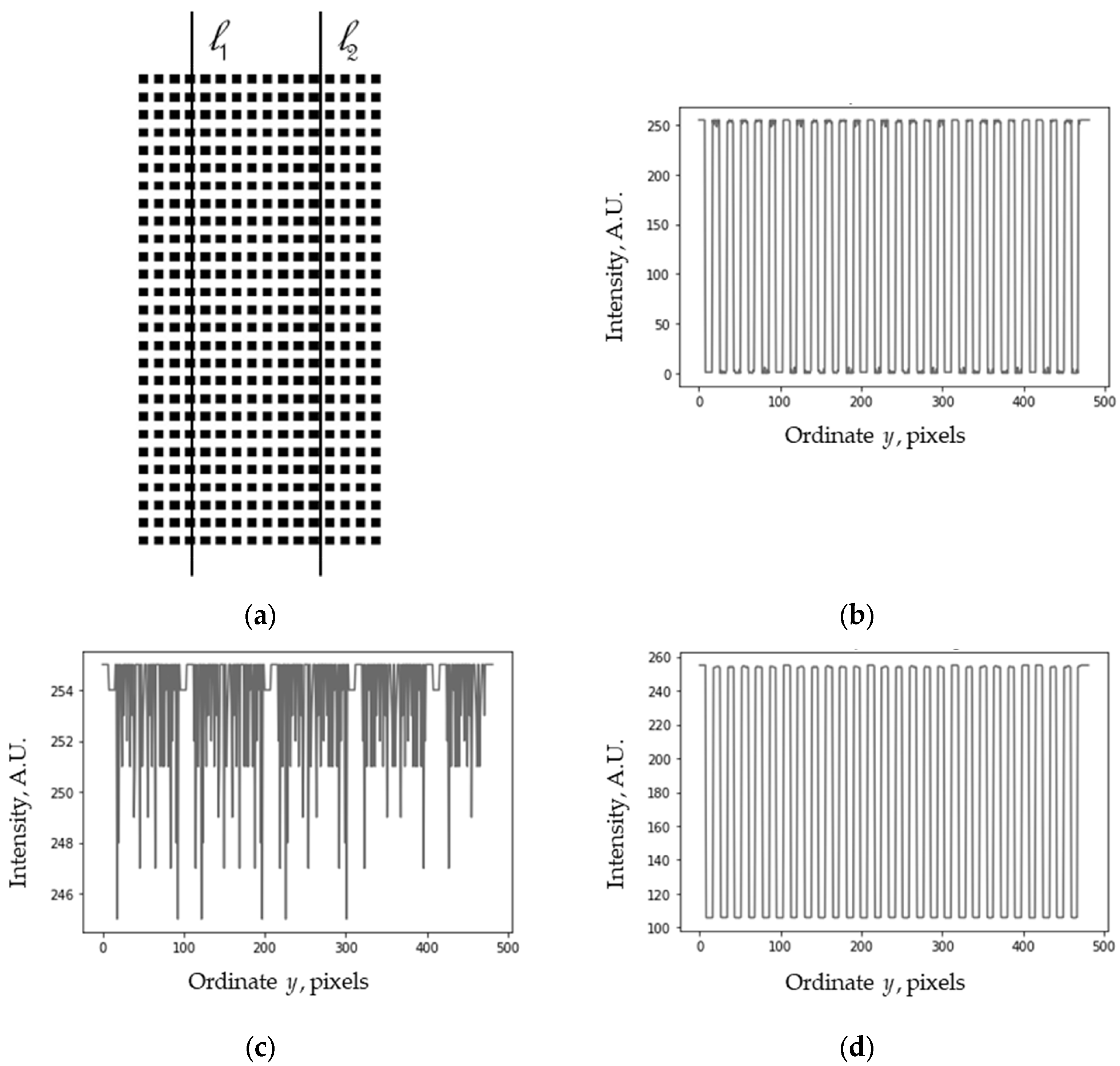
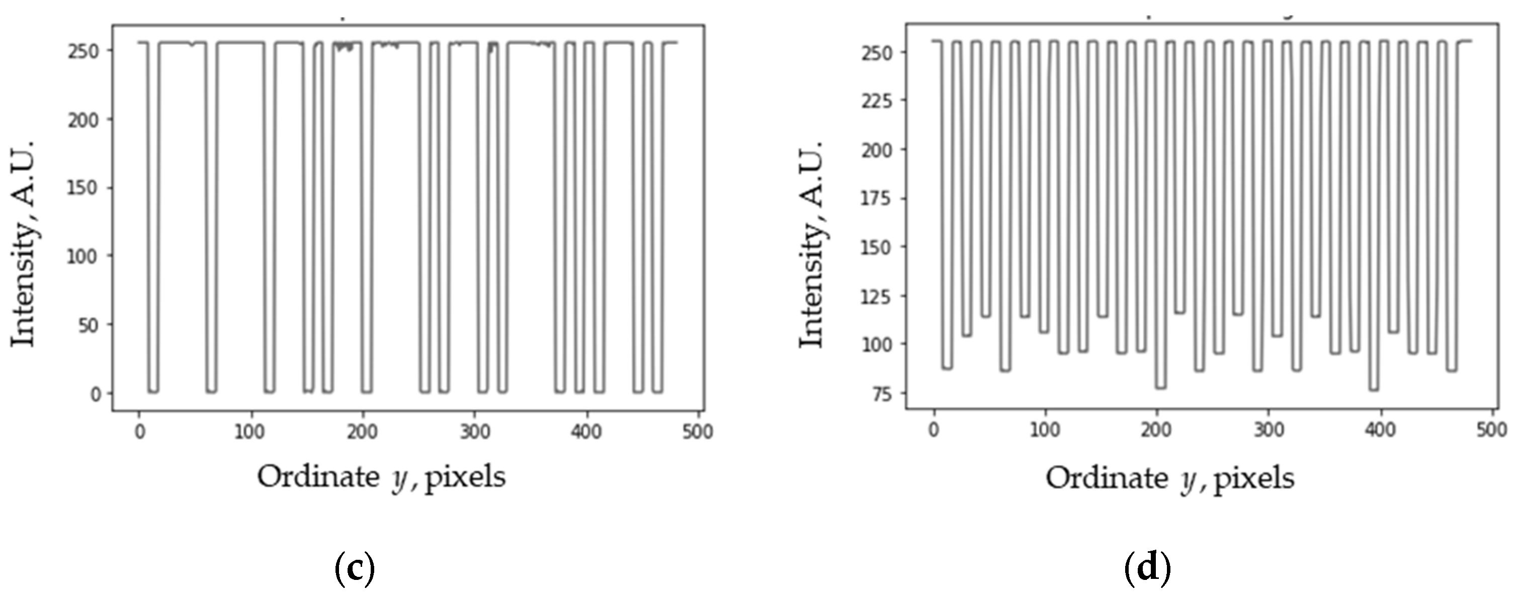
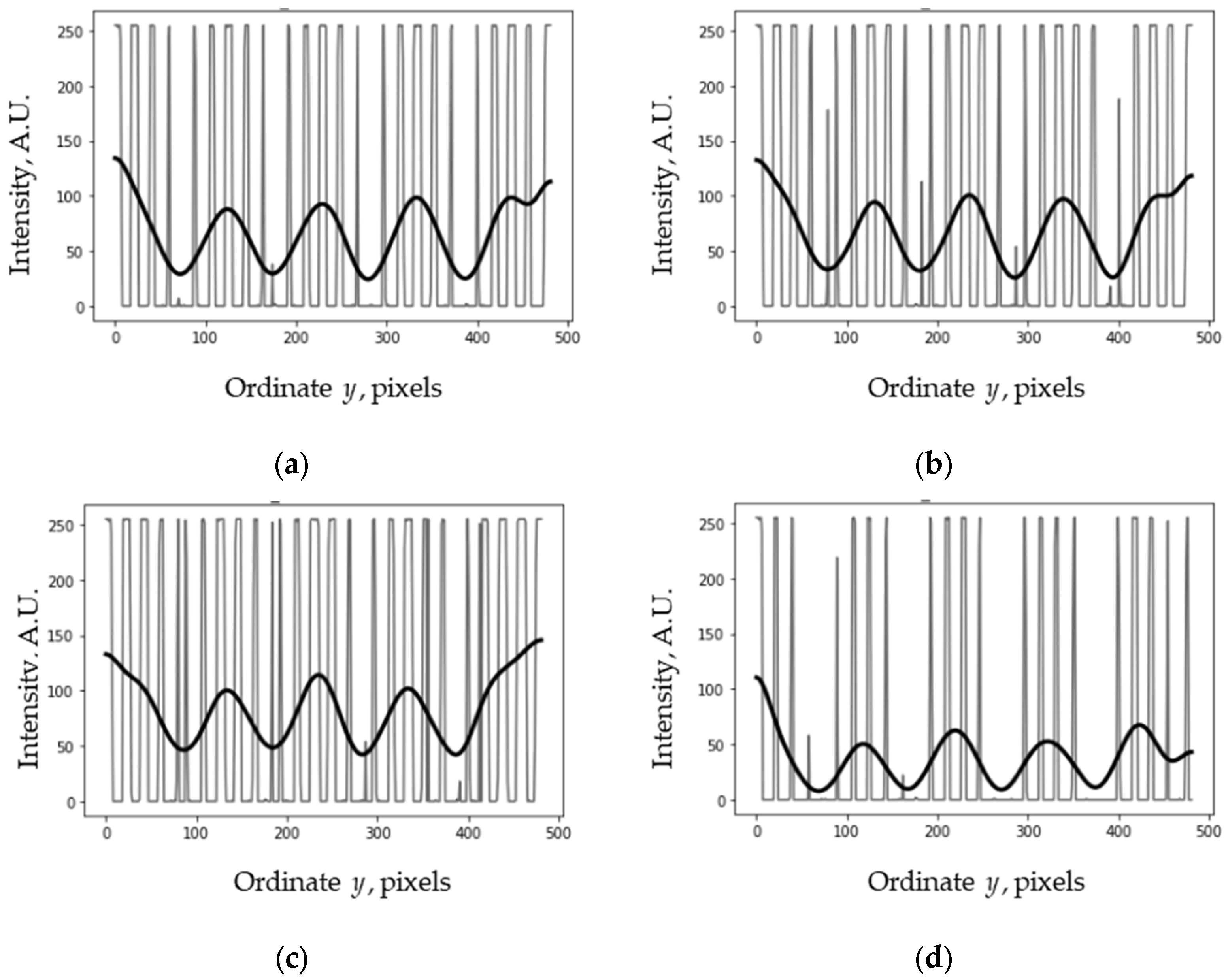
The 1D measurement method forces us to think about reducing the dimensionality from 2D to 1D. A simple way would be to use the average profile of several sections (all identical for a regular grid) for the 1D measurement. For example, the following graphical objects have identical average profiles: a linear grid with some lines shifted horizontally, and a matrix of squares with some squares shifted horizontally, as shown in Figure 4 by pairs. These examples are regular grids with rows randomly displaced horizontally (shift does not affect the average profile).

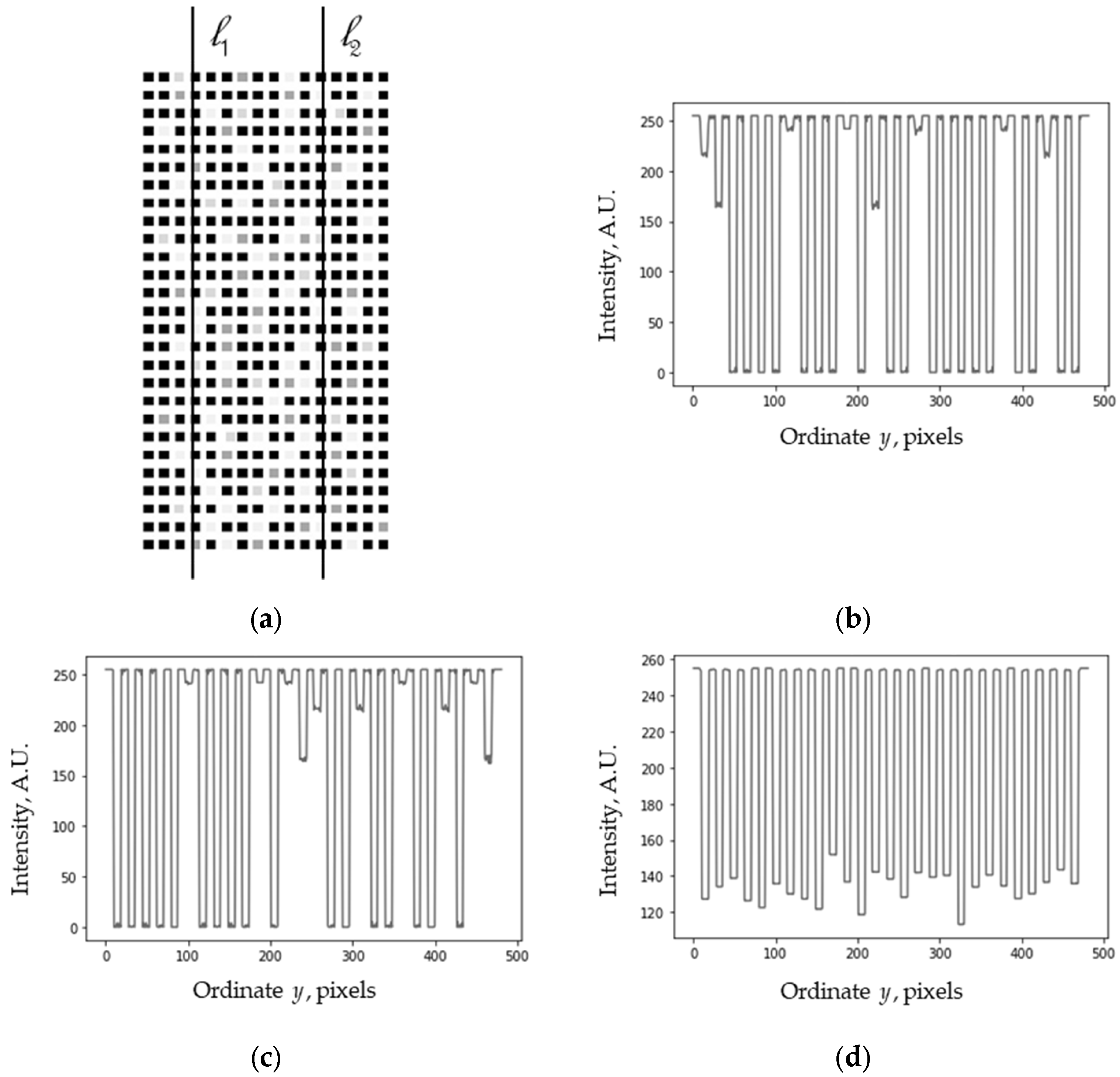
The moiré effect is an integral effect, since it can be expressed as a convolution integral [1]. Therefore, we can expect only minor differences between measurements using identical and approximately corresponding (i.e., similar) graphical objects. From this point of view, we can try to use graphical objects in which the average profile is an almostperiodic function [34]. In this case, such objects can be randomized to a higher degree; for example, they can be shifted vertically or have a changed color.

In any case, the structures should be graphically similar to parallel, equally spaced rows and have approximately the same length, height, and mean value; the variations in the average profile should not be significant. More generally, the rows should be arranged almost periodically; i.e., the vertical average profile should have one dominant spectral component (e.g., after the FFT transformation). The horizontal average profile has almost no restrictions (it can be close to constant or almost periodic).

To obtain the maximum contrast of the moiré patterns, the “opening ratio” of the average profile should be about 1/2, according to [35]. The opening ratio is the ratio of the interval between the lines of the grid to its period.

The average profile does not necessarily have to be close to a rectangular pulse function (as in the case of a regular linear grid). It can be trapezoidal, sinusoidal, or almost periodic.

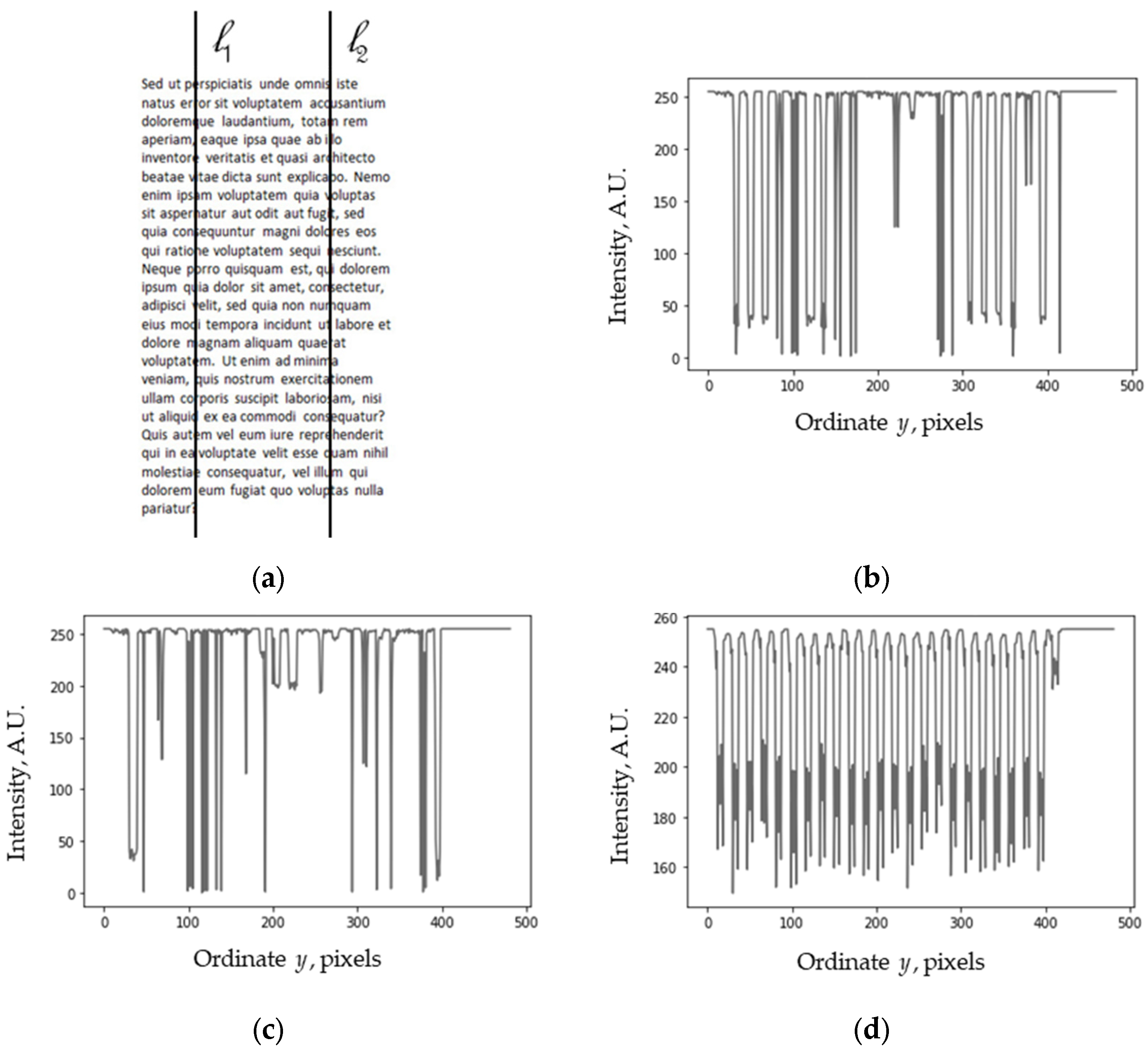
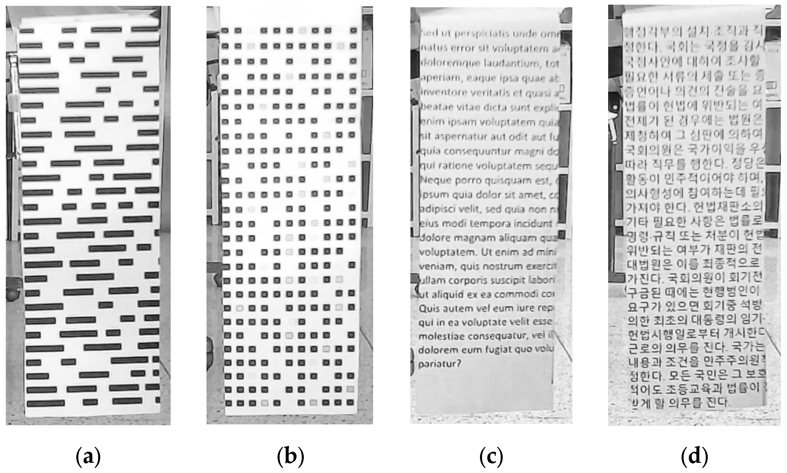
Using an almost periodic average profile allows us to take some non-ideal graphical objects, such as grids with partially worn paint or other graphical objects already existing on structures whose vibrations will be measured. Examples of such graphical objects are provided in Section 3.

2.4. Angular Alignment

A translational misalignment (horizontal or vertical) does not affect the measurements, so we considered only angular misalignment.

Figure 5 illustrates a misaligned measurement line (scan line) on a line grid with zero (or infinitely) line widths. The scan line is displayed as a line with an arrow.

The number of intersecting lines is the same in both cases: for ideal (the vertical line with the arrow in Figure 5) and imperfectly aligned (the inclined line in Figure 5) lines. The width of the lines can affect the result, but qualitatively, the angular misalignment is of little importance on a line grid, unless the scan line extends beyond the edge of the grid.

Next, consider the matrix of points of zero (or infinitely small) size, as shown in Figure 6.

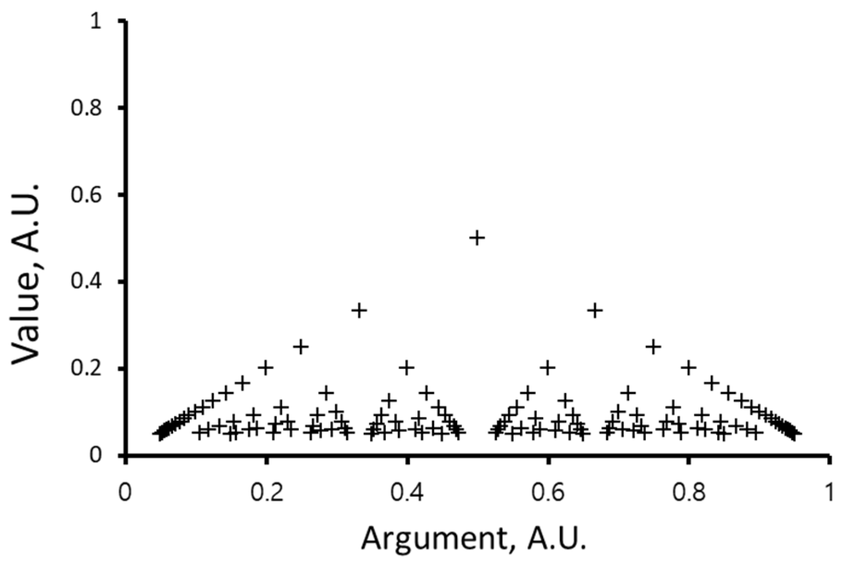
In this case, the number of intersection points, depending on the angle, will follow Thomae’s function [36], defined as follows:

$$T\left(x\right)=\left\{\begin{array}{c}0, \mathrm{for} x \mathrm{irrational}\\ {\displaystyle \frac{1}{q}}, \mathrm{for} x \mathrm{rational}(x={\displaystyle \frac{p}{q}})\end{array}\right.$$

(5)

which is sometimes called the modified Dirichlet function or the ruler function (see Figure 7).

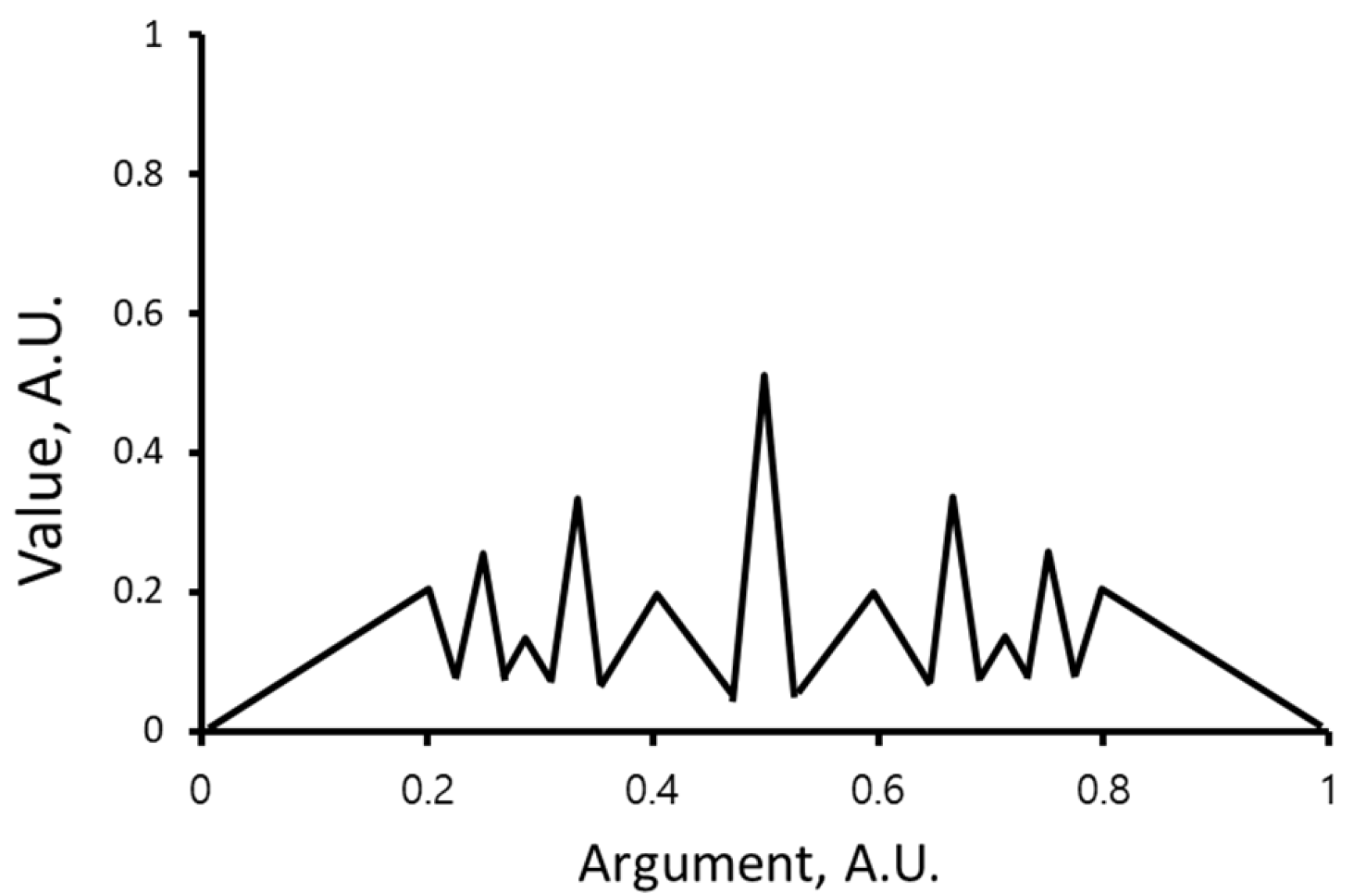
Thomae’s function is discontinuous everywhere, and its peaks have zero width. We assumed a zero size of the points; for larger (finite) sizes, the peaks expand, and their width is approximately determined as follows:

$$w={\displaystyle \frac{d}{l}}$$

(6)

where d is the size of the point, and l is the distance from the origin to the first point on the ray.

Equation (6) defines the width of the central peak; the others overlap and merge with their neighbors. Thus, for finite-size points, the intersection function has peaks of finite (non-zero) width, as shown qualitatively in Figure 8. Both types of peaks are strongly dependent on the angle, making the square grid somewhat incomparable to the line one for practical measurements.

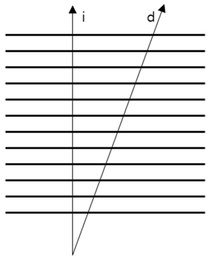
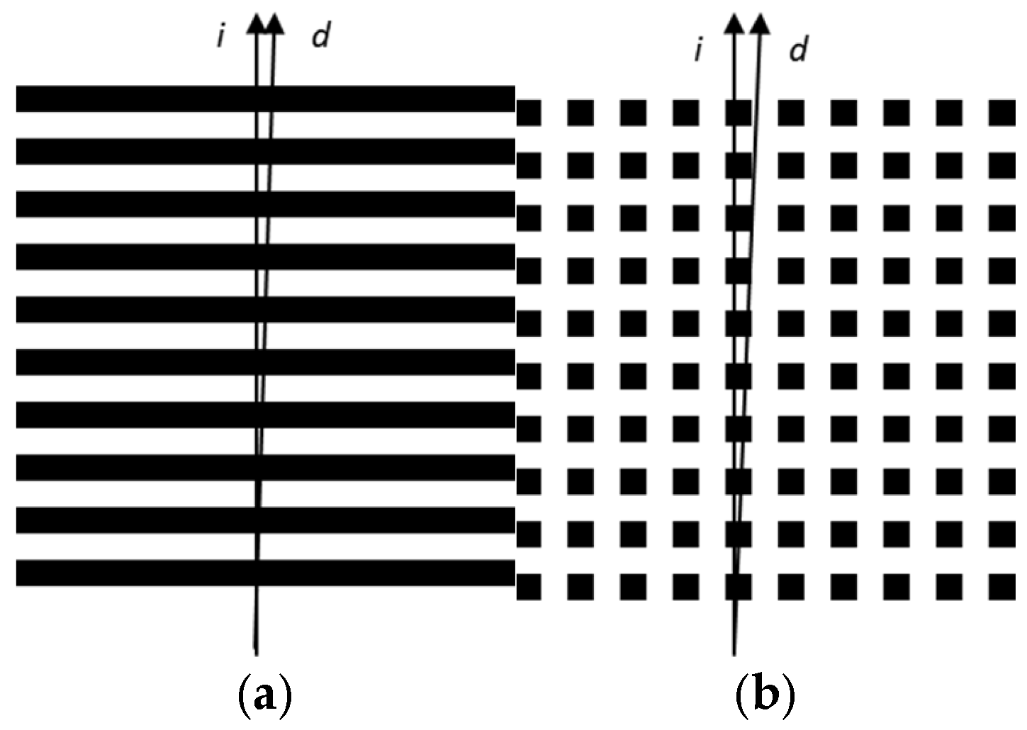
In the measurements, the operations are performed along the vertical line. At a certain misalignment, there is practically no difference between the processing along the vertical ideal (denoted as “i”) and inclined deviated (denoted as “d”) lines in the line grid (see Figure 9a). However, the dot matrix (e.g., a square matrix) requires more accurate angular alignment than the line grid due to the non-zero peak width. For example, when the scan line leaves the square at the other end of the dot matrix at an angle of approximately arctan (1/2n) (n is the number of squares) (see Figure 9b), a sharp change in intensity may occur. In subsequent processing, this may lead to a shift in the intensity of the moiré pattern and then to an incorrect measurement.

Therefore, the proposed method (using the average profile) requires an alignment accuracy similar to that of the square matrix, i.e., the allowed misalignment within the angle arctan (1/2n), because the processing is made in the horizontal direction too.

2.5. Measurement System

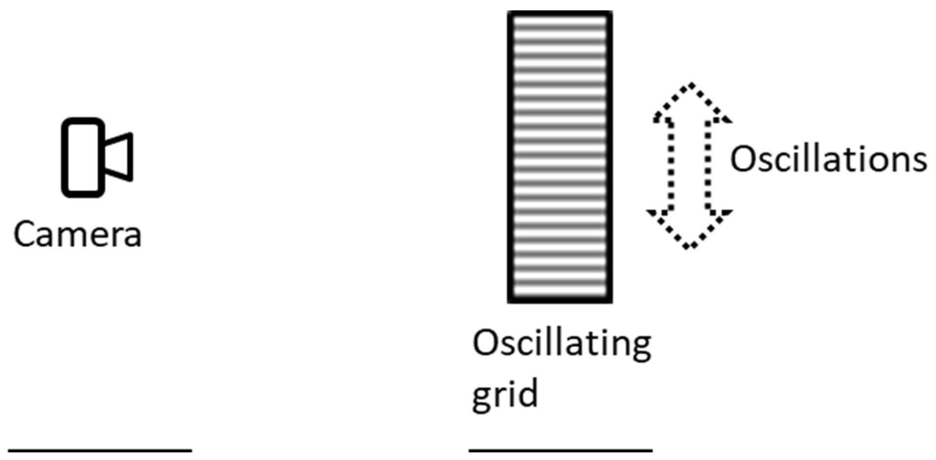
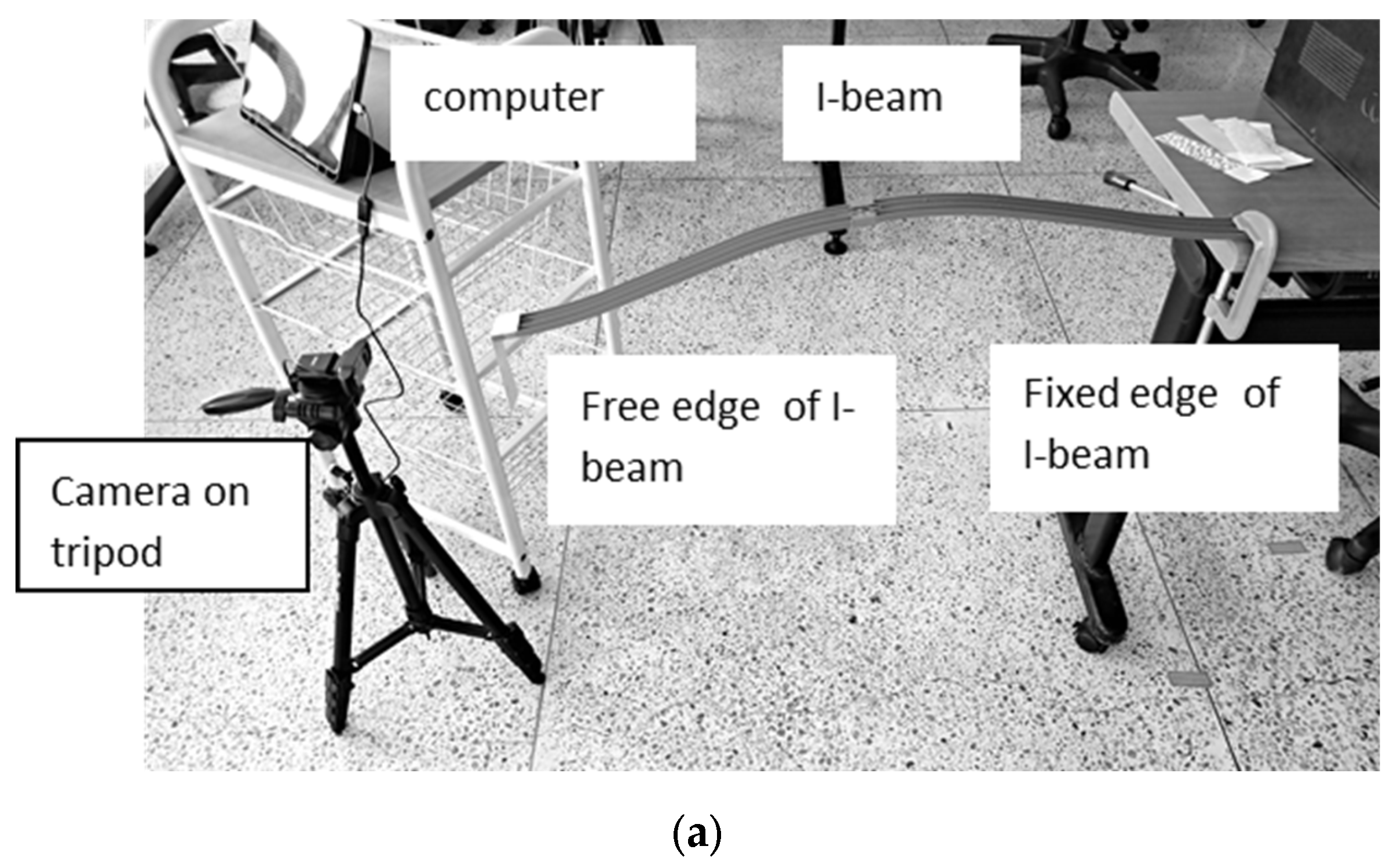
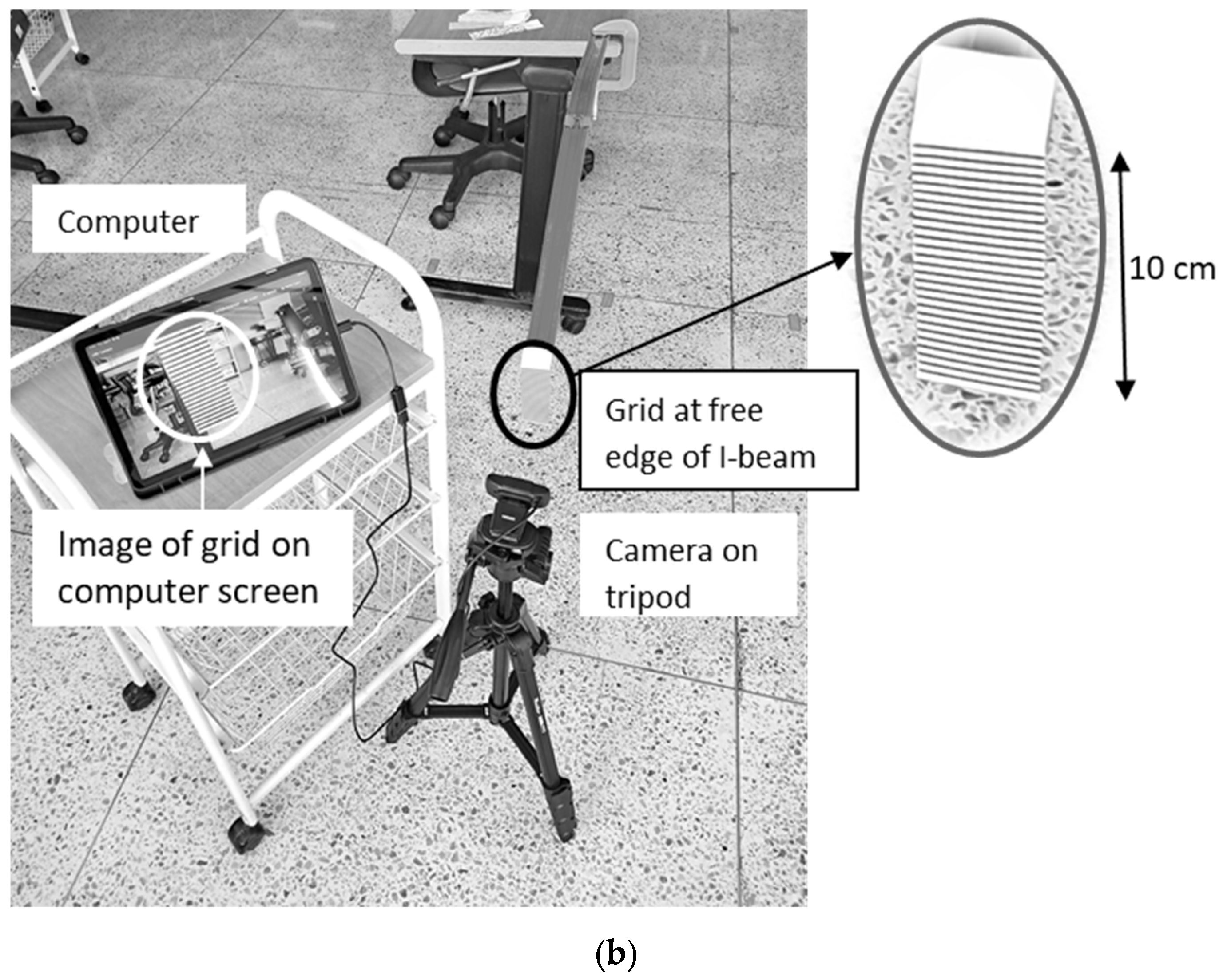
In the moiré measurement system, a grid is attached to an object whose displacement (oscillations, vibration) is measured. The camera is installed at a certain distance from the object, as shown in Figure 10. The phase of the moiré patterns is linearly proportional to the grid displacement. The physically measured value is the difference between the heights of the camera and the grid (the vibration averaged over the grid area). It is effectively applied to the center of the grid. In the system [31], a static computer-generated grid provides a common reference throughout the video.

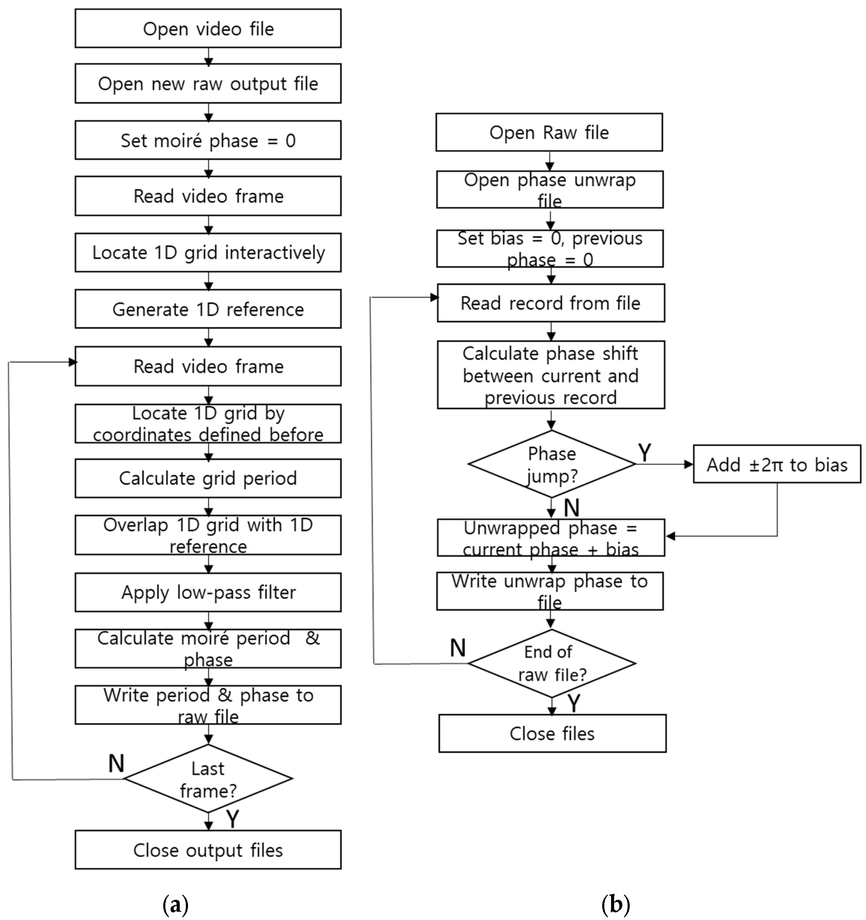
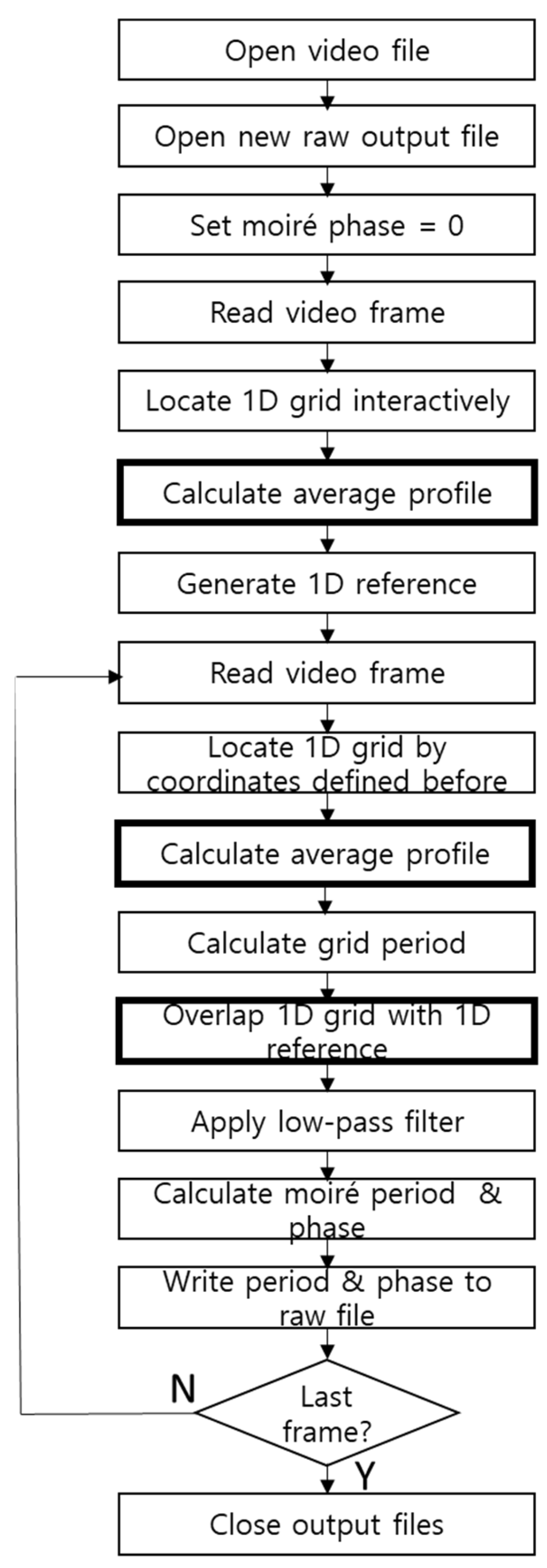
Figure 11 shows the flow charts of the processing algorithms (two stages). In the deferred system, the second stage starts after the completion of the first stage, but in the real-time system, they run simultaneously.

In the startup process (see upper part of Figure 11a), the first video frame is displayed in a pop-up window, and the start and end points of the cross section are located in the image interactively. Accordingly, we generate a common 1D reference (array) for the entire video. These points will be used for all the video frames one by one. Then (lower part of Figure 11a), we read all the video frames and superimpose the cross section of the current grid (using the points defined in the startup) with the reference. The product is filtered using a Gaussian filter, and moiré patterns are obtained. Their period and phase are measured and written to the raw file. In the second stage (see Figure 11b), the raw phase is unwrapped by adding/subtracting the period corresponding to the sign of the detected phase jump between the current and previous frames, as in [37]. The result is written to the file (deferred version of the system) or displayed on the screen (real-time version).

3. Results

Previously [31], we considered grids with a rectangular profile consisting of solid straight lines, shown in Figure 12a. The grid’s intensity profile, i.e., its cross section along a line (l) perpendicular to the grid lines (in this example, vertical), is shown in Figure 12b (the intensity was measured in 8-bit units from 0 to 255). The profile is the same for all the parallel vertical lines within the grid.

3.1. Approximate Grids

Except for the line grid, other regular graphical objects, such as a dot matrix, shown in Figure 13a, can also be used for the moiré effect. However, in this case, the profiles along different lines are different (see Figure 13b,c). Such an inconvenient irregularity makes dealing with the vertical profiles difficult.

To eliminate the influence of such irregularity, we consider the average profile obtained by summation along the horizontal lines of the image, as shown in Figure 13d. Such a profile does not depend on the horizontal coordinate.

Besides regular grids, we can also consider some nearly regular graphical objects arranged in rows. For example, the pattern in Figure 14a consists of segments of straight lines lying at the same height in each row. Also, some of the black squares of the square grid shown in Figure 13 can be recolored or even removed, as in Figure 15a. In these cases, the profiles along different lines are already different (see Figure 14b,c and Figure 15b,c). However, the periodic structure can be recognized in the average vertical profiles (obtained by summation along the image lines), shown in Figure 14d and Figure 15d.

The average profiles are not strictly periodic but are nevertheless close to it. In these cases, the average profile is an almost periodic function. Later, we will see that such a “distorted” periodicity may almost not affect the moiré measurements.

3.2. Other Graphical Objects as Grids

As an illustration of the flexibility of the proposed approach, consider some other graphical objects arranged in “rows”, such as text, which can also be used for the moiré effect (see Figure 16a). An excerpt from a dummy placeholder text called “lorem ipsum” is shown in Latin in [38]. Again, although the cross sections are different (Figure 16b,c), the average profile (Figure 16d) is close to periodic, except for some narrow peaks. This situation is generally similar to the dashed lines or the gray-dot matrix, although the average profile of the text is less regular.

Usually, the text in other languages is also arranged in parallel rows (see the example of lorem ipsum in Korean [39] in Figure 17) and thus can also be used for the moiré effect. The Korean language was taken as an example of a language whose writing system is not based on the Latin alphabet. As before, while the individual profiles (cross sections) shown in Figure 17b,c are different and almost random, the average profile appears close to regular (especially its “upper” part), and its almost periodic structure is recognizable.

All samples in Figure 13, Figure 14, Figure 15, Figure 16 and Figure 17 are arranged in rows; i.e., they consist of parallel, horizontal, relatively dark “rows” separated by blank gaps, although within the rows, they may be unpredictable and almost random. The vertical cross sections of such grids are practically random functions, and the moiré patterns obtained from these profiles will also be random. However, the average vertical profile (obtained by summation along the image lines) is almost periodic, and the periodic structure is recognizable. Therefore, their average profiles help obtain a uniform moiré effect independently of the internal almost random structure inside the “rows” and can therefore be used for the moiré measurements as a 1D cross section of the grid, similar to Section 2.

3.3. Computer Simulation

To verify our approach (using graphical objects arranged in rows), we primarily simulated the moiré effect in the four grids considered in Section 3.1 and Section 3.2 (i.e., dash grid, grayed square grid, Latin and Korean text). All grids had the same period. As in Figure 1, the product resulted from the multiplication of the average intensity profile with the reference, and the moiré patterns were obtained as filtered products (namely, the Gaussian filter with the standard deviation of 15 units). The results of the simulation are shown in Figure 18.

The shape and period of the moiré patterns are practically identical in all four cases. Although the patterns near the cross section edges are somewhat distorted, the periods in the middle were 106.5, 106.5, 104, and 104 units; the average period was equal to 105.25, very close to that of the regular line (see the Section 1). This suggests that grids arranged in rows can be successfully used.

3.4. Measurements Using Various Grids

The measurement scheme was similar to that shown in Figure 10; the general view (photographs) is shown in Figure 19. The grid was attached to the free edge of the I-beam.

We used a Samsung Galaxy Tab S9 FE (10.9″) tablet computer and an external webcam on a tripod in the experiments. The plastic rod (I-beam) length with one fixed edge was 88 cm, and its cross section was 37 mm × 8 mm. A C-clamp held one edge of the rod on the table; the grid was attached at the free edge. The distance from the camera to the free edge of the rod was 25 cm. The size of the printed grid was 4 cm × 10 cm, and its period was 4.038 mm.

The vibration was excited by manually pushing the I-beam (using a similar plastic rod) approximately in the middle. The FHD video (1920 × 1080, 30 frames per second) was recorded for about 1 min. The grid image’s typical size was 480 × 260 pixels. The grid image can be seen on the computer screen shown in Figure 19b.

The regular line grid was processed according to the algorithm described in Section 2. In the measurements in grids other than the line grid, the average profile was used instead of the profile. Figure 20 shows the first stage of the image processing algorithm modified for the average profile of graphical objects arranged in rows. Almost all the steps of the image processing algorithm (including the superimposition with the computer-generated grid and the measurement of the phase of the moiré patterns) remained exactly the same as those for the regular line grid described in Section 2. The modified sections are outlined in Figure 20 in bold. The phase unwrapping algorithm remained untouched.

Figure 21 shows examples of photographed grids arranged in rows. Figure 22 illustrates the stages of processing.

The period of oscillations was measured as the time interval between the successive maxima or minima on the time plot shown in Figure 22c, and the amplitude (Figure 22d) was measured as one-half of the peak-to-peak magnitude (between the current maximum and the following minimum on the time plot). The exponential regression of the amplitude gives the logarithmic decrement of the decayed oscillations.

3.5. Analysis of Measurements Using Various Grids

The results of the measurements using a regular grid and other graphical objects arranged in parallel rows are presented in

Table 1. Summarized results of measurements of decaying oscillations in I-beam.

Grid	Period, s	Standard Deviation	Decrement, s−1	R2 (Coefficient of Determination)
Mean	0.493	4.2%	−0.107	0.984
Standard deviation	0.001		0.024
NRMSE	0.27%		22.74%

,

Table 2. Results of measurements of decaying oscillations in I-beam by groups.

Grid	Period, s	Standard Deviation	Decrement, s−1	R2 (Coefficient of Determination)
Line	0.494	3.6%	−0.128	0.965
Dash	0.494	3.5%	−0.103	0.997
Square	0.493	4.6%	−0.095	0.973
Partially grayed square	0.493	4.2%	−0.113	0.994
Latin text	0.495	4.6%	−0.119	0.985
Korean text	0.492	4.4%	−0.093	0.988
Mean	0.494	4.2%	−0.108	0.984
Standard deviation	0.001		0.014
NRMSE	0.24%		12.74%

and

Table 3. Results of measurements of decaying oscillations in I-beam for selected videos.

Grid	Period, s	Standard Deviation	Decrement, s−1	R2 (Coefficient of Determination)
Line	0.495	3.4%	−0.094	0.993
Dash	0.494	3.5%	−0.100	0.998
Square	0.493	4.0%	−0.104	0.987
Partially grayed square	0.492	4.9%	−0.107	0.989
Latin text	0.495	5.6%	−0.111	0.986
Korean text	0.492	3.7%	−0.107	0.995
Mean	0.494	4.2%	−0.104	0.991
Standard deviation	0.001		0.006
NRMSE	0.29%		5.87%

. We processed 19 individual videos (six grids, 2 to 4 videos for each grid). The statistical data for all 19 measurements with no regard for the grid type are given in Table 1. The normalized root-mean-squared error (NRMSE) is a measure of the accuracy; it is equal to the ratio of the standard deviation to the range of the variable and is expressed in percent. The coefficient of determination (R²) shows the quality of the regression. For videos divided into six groups (according to the grid type), the data are given in Table 2. For the six selected files (only one video with the best R² from each group), the data are provided in Table 3.

The mean period is practically the same in all three cases (Table 1, Table 2 and Table 3), and its NRMSE (derived from the standard deviation) is less than 0.3%. This means that the differences in the measured period between the groups and the individual measurements in all the tables are negligible. The mean decrement is also nearly the same in three cases, but its variation is over 5%, and it exceeds 20% in the first case (Table 1).

The experiments showed the following: the mean measured period (across all grids) was 0.494 s, the average decrement was −0.104 s⁻¹, and the oscillation frequency was 2.024 Hz with an average lifetime of 9.615 s. There was no difference between the period of oscillation measured using the linear grid and the period measured using other graphical objects. The NRMSE of the period (across all grids) was less than 0.3%, the NRMSE of the decrement was less than 6%, and the determination coefficient of the exponential regression (R²) was over 0.986 (i.e., 98.6%). Such values of the NRMSE and R² mean that the results of the measurements using all grids are similar. These experiments demonstrated the reliability of moiré measurements using the average profile of various graphical objects arranged in rows.

4. Discussion

Moiré measurements for graphical objects arranged in rows were obtained using the average profile. They appear similar primarily because of the integral nature of the moiré effect. Thus, the influence of narrow peaks mentioned in Section 3.2 was effectively eliminated.

However, a more precise angular alignment was required in the approximate grids and text compared to the regular linear grid.

We considered only five examples of graphical objects arranged in rows. However, many similar graphical objects can easily be found around us, for example, in slogans, labels, advertisements on bridges, buildings, equipment, and the like, and are accordingly used in practice with the processed average profile.

Changing the frequency does not affect the measured displacement, but it can affect the period. This can happen in the processing of a recorded video, since it assumes equidistant frames. However, this factor can be eliminated in real-time processing because, here, we can rely on other methods of measuring the time intervals, for example, using the operating system calls.

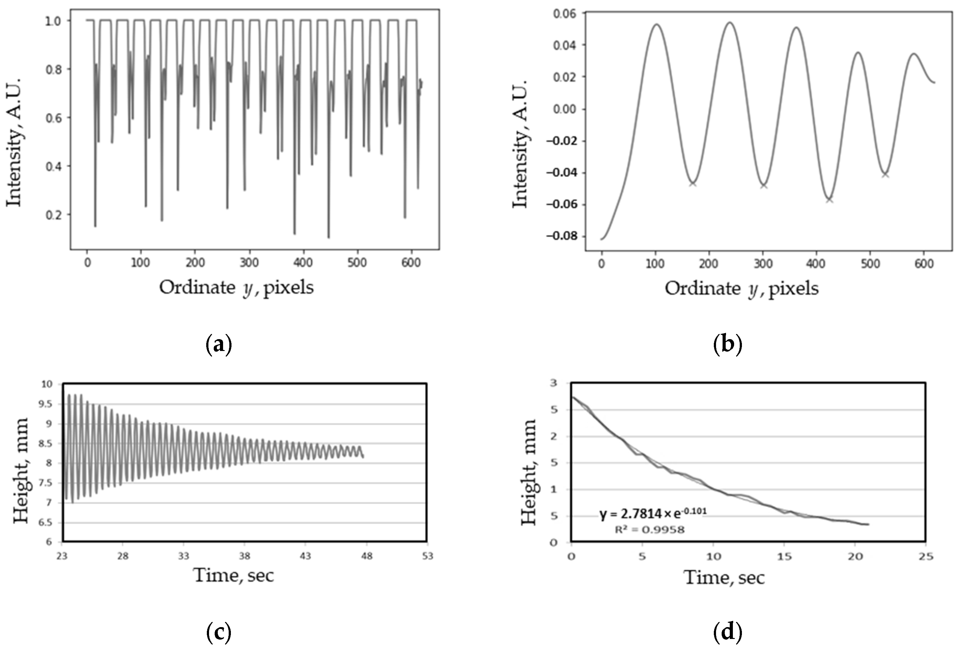
As described in Section 3.4, the period of oscillation was measured as the distance between the successive maxima or minima on the time curve. We did not compare the measured values at each point of every waveform in each experiment; instead, we compared the secondary parameters (period and decrement) that are independent of the particular time curve.

The mechanical properties of the rod’s material determine the period and decrement. We used the same rod of the same length in all the measurements presented in our paper. The experimental setup remained untouched after assembly until all the experiments were completed. In practice, the values of the period and decrement deviate slightly due to natural causes; unavoidable noise caused some deviations. However, the method for measuring the decrement (currently, the exponential regression) should be improved, since it has a larger deviation.

It might be worth trying to take measurements using the average profile without the moiré effect, but we have not yet performed this.

The algorithm in Figure 11 has been additionally implemented in real time [40]. In this case, both stages of the algorithm (measuring the moiré phase and unwrapping it) were implemented in one pass. As there is no significant difference between the original algorithm and the algorithm modified for graphical objects arranged in rows (Figure 20), there are no principal restrictions on the modified algorithm’s implementation in real time.

5. Conclusions

We investigated the moiré effect in graphical objects arranged in parallel rows. Despite the completely different (virtually random) results that could be obtained with conventional image processing, very similar results were obtained in various grids with a slight change in the processing algorithm (using the average profile). The similarity was demonstrated for five graphical objects arranged in rows, including approximate grids and text in different languages. The results can potentially be applied to practical moiré measurements using graphical objects arranged in rows that may already exist on the object.