Measuring Salinity and Density of Seawater Samples with Different Salt Compositions and Suspended Materials

Abstract

Determining the solute mass amount in seawater using in situ measurements in seas and oceans is currently an unresolved problem. To solve it, it is necessary to develop both new methods and instruments for measurements. The authors of this article analyzed methods for the indirect measurement of salinity and density using parameters that can be measured in situ, including relative electrical conductivity, speed of sound, temperature, and hydrostatic pressure. The authors propose an electric conductivity sensor design that allows for the obtainment of data on solid suspensions along with measuring the impedance of electrodes under various the alternating current frequencies. The authors analyzed the joint measurement technique using the Conductivity-Temperature-Depth (CTD) and Sound Velocity Profiler (SVP) devices in a marine testing area. Based on the results of joint measurements, the authors present tests of water samples of various salt compositions for the presence of solid suspensions.

1. Introduction

Knowledge of salt composition and suspended matter is a prerequisite for forecasting and developing marine ecosystems. The influence of salinity on the physiological and behavioral parameters of planktonic organisms has been rarely investigated (Lee and Petersen, 2002). Living in a variable salinity mode provides a unique opportunity for individual populations to quickly acclimatize.

During marine research in the Black Sea and Sea of Azov, we conducted experiments to determine the reliability of the measurement results obtained with Conductivity-Temperature-Depth (CTD) and Sound Velocity Profiler (SVP) instruments in the shelf zone. We used the data from these experiments to calculate the salinity and density of seawater.

When studying the results of the joint measurements by the CTD and SVP devices, we identified a number of factors that signified an incorrect interpretation of the obtained data. We compared these data with the values of salinity and density indirectly obtained using well-established algorithms.

We assumed that the use of standard algorithms, which do not consider the effects of solid suspensions in the seawater, results in significant errors in the calculations of salinity and density when processing in situ measurements obtained using the CTD and SVP devices.

We must note that some researchers have been trying to develop methods for correction marine measurement results that would help to determine the true values of absolute salinity and density of seawater with non-standard composition, including samples with solid suspensions.

Some well-known works [1,2,3,4,5,6,7,8,9,10] have only partially solved this problem. For example, when determining a salinity anomaly δS_A with CTD probes with an electric conductivity measurement channel, the TEOS-10 user manual [11] suggests to use a chemical conductivity and density model [1] to assess the correlation between the salinity changes and measured properties of seawater.

This model allows for the determination of the salinity anomaly expressed in (g/kg) through nitrate (NO₃⁻) and silicate (Si(OH)₄) concentration values in a seawater sample and through the two differences of ΔTA (∆TA = Total Alkalinity (TA) − 0.0023 (S_P/35), mole/kg) and ΔDIC (∆DIC = Dissolved Inorganic Carbon (DIC) − 0.00208 (S_P/35), mole/kg):

δS_A/(g/kg) = (55.6·∆TA + 4.7·∆DIC + 38.9·NO₃⁻ + 50.7·Si(OH)₄)/(mole/kg),

(1)

where S_P is the practical salinity expressed in practical salinity units (psu). The ΔTA and ΔDIC differences are determined between the TA and DIC in a sample and the respective best assessments of TA and DIC in standard seawater [1,2].

According to [2], the standard uncertainty of model compliance is 0.08 mg/kg in the oceanic range if the exact amounts of all the substances are known.

Other research works have shown that δS_A can be calculated using a simplified empirical equation based on the measurement of SiO₂ silicate concentration measurement and the total alkalinity (TA) because these components are measured and well-suited for the assessment of density and salinity changes of the deep water.

This empirical equation is as follows [3]:

δS_A = a·∆[SiO₂] + b·∆[NTA],

(2)

where NTA is the total alkalinity, normalized to salinity 35 (NTA = (TA/Sp)·35).

According to Millero [4,5,6,7], ∆[NTA] is the difference between the measured value of normalized total alkalinity (NTA) and the reference value (0.0023 mole/kg) for surface seawater. However, the practical method for determining δS_A is based on the use of density measurements [8].

As stated in [3,9], the method proposed by Millero et al. can be used to calculate δS_A through the following formula: δρ = 0.75179 δS_A.

Unfortunately, the majority of results have been obtained in laboratories because it is difficult to adjust measurement results through bathometer sampling and subsequent seawater density measurements onboard a ship when using, for instance, an Anton Paar DMA 5000 M vibration sensor because the task of keeping of solid suspensions in suspension state in a sample is not easy.

It is difficult to use these models and research works when working in situ in the shelf zone where there are solid suspensions.

2. Materials and Methods

As mentioned above, our research was conducted in the natural conditions of the shelf zone using two devices and one model.

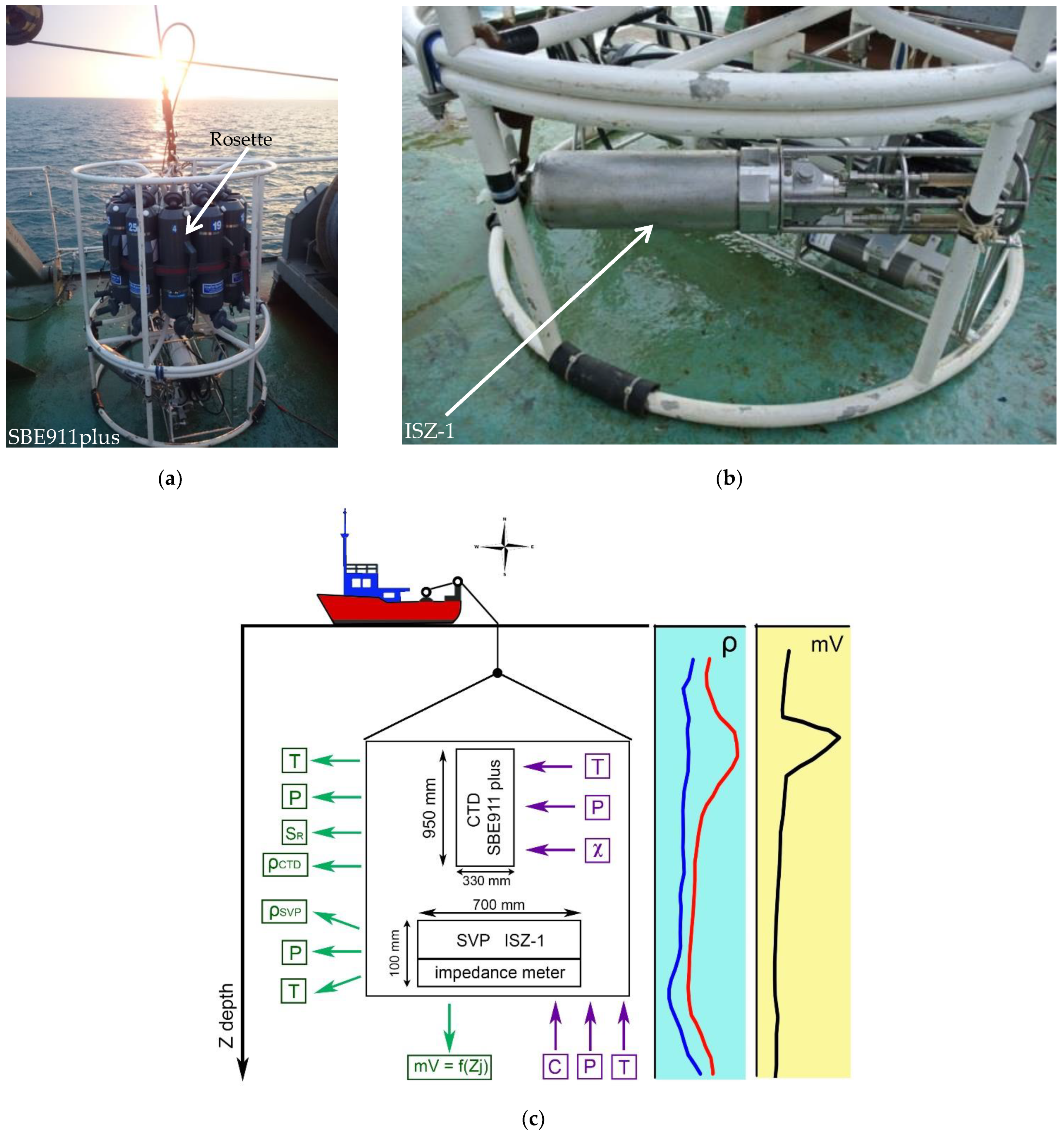
To do this, we complemented a standard SBE911 oceanological probing CTD unit [12] with an ISZ-1, which is an SVP probe developed at the Institute of Natural and Technical Systems (INTS) [13] (Figure 1). The ISZ-1 probe also featured an ultrasonic attenuation measuring channel. Unfortunately, it only worked on a few of the stations and it ran in the testing mode. Data on the metering attenuation duct are provided in [14]. In the testing mode, an impedance channel model with the 4-electrode cell was used, and its operation is described below. Figure 1c shows a structural and functional diagram of the entire measuring set of instruments and included devices, as well as their dimensions. The devices were lowered on a cable-rope to a certain depth using a winch installed on the ship. The ship’s coordinates were fixed by navigation systems. The input measured parameters of the water are indicated in purple: T—temperature; P—hydrostatic pressure; c—speed of sound; and χ—electrical conductivity. The calculated output values are indicated in green: T—temperature; P—hydrostatic pressure; S_R—salinity; ρ_CTD—calculated density values from CTD readings; ρ_SVP—calculated density values according to SVP readings; and mV—impedance value Z_j. The same figure shows the vertical profiles of the density (ρ_SVP and ρ_CTD) and impedance distribution expressed in mV.

The specifications for both probes are presented in

Table 1. Specifications of the ISZ-1 probe.

Measured Parameters	Range Measured	Error
Sound speed, m/s	1375 … 1900	±0.02
Water temperature, °C	−2 … +35	±0.001
Hydrostatic pressure, dbar	0 … 2000	±2

and

Table 2. Specifications of the SBE911plus probe.

Measured Parameters	Range Measured	Error
Electric conductivity, S/m	0 … 7	0.0003
Water temperature, °C	−5 … +35	0.001
Hydrostatic pressure, dbar	0 … 2000	0.015%

.

Both devices were mounted on the same basket next to one another, which allowed us to compare measurement results based on two different salinity and density calculation methods using electric conductivity or sound speed. When calculating density and salinity using the data measured by the CTD probe, we used the integrated SeaBird software based on TEOS-10.

When reviewing measurement results obtained using the CTD and SVP devices to determine the causes of discrepancies, we also analyzed the measurement channels for electrical conductivity and sound speed in the seawater. Two other measurement channels (pressure and temperature) were identical in their metrological parameters. To compare the discrepancies in the measurements obtained using the CTD and SVP devices, we compared the values of salinity and density calculated by the algorithms based on TEOS-10 and that have been established for clear seawater without impurities. Next, we review in detail what factors affect the reliability of measurements obtained through in situ devices by analyzing the operations of measurement channels for sound speed and electrical conductivity.

CTD probes widely employ the contact (conductive) method and the contactless (inductive) method to measure the specific electrical conductivity of water. For example, conductive sensors are used in devices such as Neil Brown Instrument Systems (NBIS), Sea Bird Electronics Inc (SBE), Guildline Instruments Ltd. (Guildline), and IDRONAUT S.r.l. Inductive sensors are used in Aanderaa Data Instruments AS, Falmouth Scientific, Inc, and other devices. Despite their advantages (zero contact), inductive sensors have a narrow frequency bandpass, and it is very difficult to extend their functional capacities, e.g., in order to use them for impedance spectroscopy.

The most successful conductive cells have four electrodes or more. Electrodes are made of platinum and located inside an alumina ceramic or borosilicate glass cylindrical tube. For example, a Sea Bird Electronics Inc (SBE) cell is equipped with 10 mm wide platinized round electrodes and a 190 mm long tube, with an internal diameter of 7 mm.

The design features of the cells and their shielding are well-developed in modern devices; therefore, the influence of external fields is minimized. As a consequence, the effect of interference on the cell is reduced, which contributes to good metrological characteristics. However, the large cell length and a small cross-section of the flow channel make it impossible for water to pass through the cell with the required speed. Thus, forced injection systems (special pumps) are used in this case. The small diameter of the flow channel makes SBE probes very sensitive to impurities.

When electric current passes through a conductive cell, a chain of electric and thermodynamic processes starts in it.

When the current is not supplied to the electrodes, the ions in the solution only take part in thermal motion. When a field of strength E is supplied on a cell, it forces the ions to move towards the electrodes, complementing the thermal motion.

The key problem with conductivity measurement using alternating current is the correct interpretation of the results. This can be complicated by the facts that the equivalent circuit of a cell is usually unknown and that the sample with connected electrodes is basically an electric black box.

When studying the impedance of electrochemical cells, it is necessary to obtain reliable information on electrode processes, i.e., the processes occurring on the surface of contact between the electrode and electrolyte.

Let us review in detail a conductive sensor with 4-electrode cell.

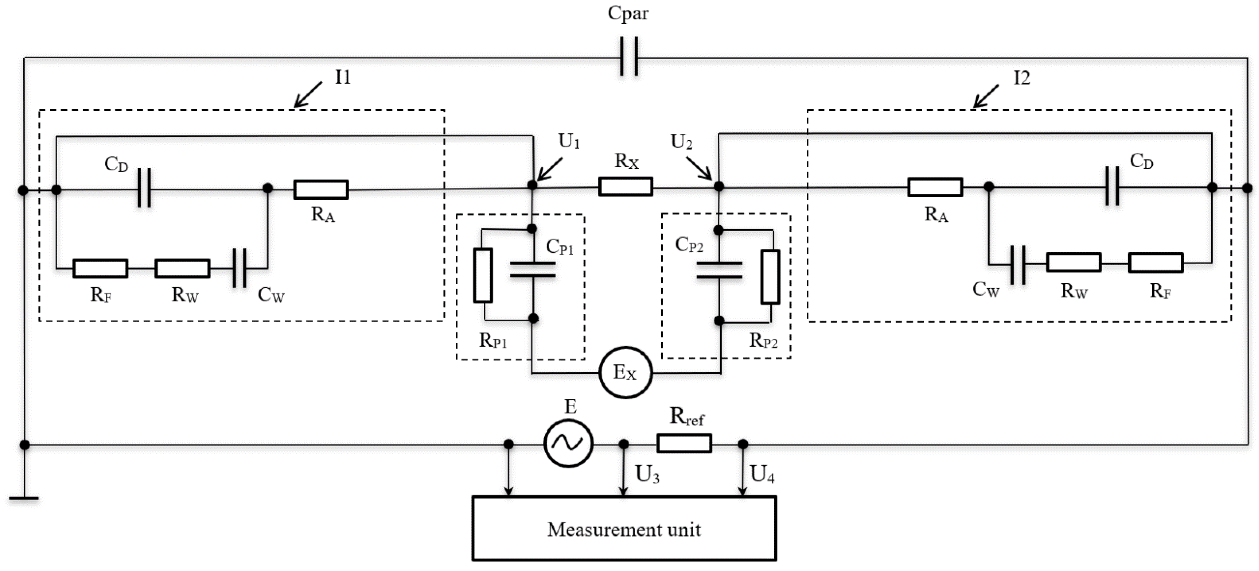
The equivalent circuit of a 4-electrode cell with an auxiliary node to measure impedance is shown in Figure 2.

The equivalent circuit of the cell in question comprises two current (I1 and I2) and two potential (U1 and U2) electrodes with some of the impedance of the water solution in question between them. Current electrodes I1 and I2 are supplied with alternating current. They can be represented as a capacitance of double layer C_D, parallel with the impedance of electrochemical polarization $R_F=\partial E/\partial i_F$ and serial-connected to resistance R_W and capacitance C_W related to the concentration polarization (usually referred to as Warburg’s impedance) [15].

Resistance R_A reflects the absorption of atoms, ions, or molecules on the surface of the electrode, and it can be equal to zero under appropriate conditions (e.g., the use of a perfectly polarizable electrode and an inert electrolyte).

In an equivalent circuit, parasitic capacitance Cpar accounts for a sum of capacitances determined by the dielectric constant of water solution, the distance between the electrodes, the active surface areas of electrodes, and the capacitance between the conductors connected to the electrodes. When considering impedance, it is worth noticing that the parasitic capacitance is especially evident at higher frequencies. For the equivalent circuit shown in Figure 2, the total impedance of the conductometric cell in question can be expressed as follows, provided that Cpar = 0:

$$Z_j=R_X+\frac{2R_W{C}_W^2}{{\omega }^2{R}_W^2{C}_W^2\hspace{0.17em}{C}_D^2+{(C_D+C_W)}^2}-2j\frac{{\omega }^2{R}_W^2{C}_D{C}_W^2+C_D+C_W}{{\omega }^2{R}_W^2{C}_W^2{C}_D^2+{(C_D+C_W)}^2}\cdot \frac{1}{\omega }.$$

(3)

In this expression, the first component is the true impedance value of solution, the second real component can be denoted as ΔR_W is the error caused by polarization phenomena, and the third component is the virtual one that can be determined as capacitive reactance.

This can be reduced by using special circuits integrated into the measuring device and used to obtain additional information on the phase at various frequencies, which can be further used in the research of cell impedance variability. We know that the material and surface condition of electrodes have significant impacts on the polarization impedance value. We assume that the value of polarization impedance is related to the design of the crystalline grid of the electrode material, the absorption properties of its active surface, and the formation of surface oxidic films. Additionally, the frequency of alternating current has a significant impact on the polarization effect. Numerous authors [16] have claimed that the correlation between R_W and frequency for reversible electrodes made of different materials used in water solutions of various concentrations can be expressed as follows:

$$R_W=\frac{\eta }{\sqrt{\omega }}$$

(4)

where $\eta$ is a constant. From Formula (4), we can conclude that R_W decreases as the frequency increases and becomes insignificant at frequencies above 1 kHz. On the other hand, the correlation between the polarization capacitance and the frequency is as follows:

$$C_W=\frac{1}{\eta \sqrt{\omega }}$$

(5)

The constant $\eta$ in expressions (4) and (5) reflects the dependence of R_W and C_W, respectively, from concentration, ion diffusion factor, and double-layer potential.

$$\eta ={\displaystyle \sum _i{\beta }_i\hspace{0.17em}{\nu }_i}\frac{1}{\sqrt{2D_i}},$$

(6)

where ${\beta }_i=\frac{\partial E}{\partial W_i}$; $W_i$ is the concentration of the potential determining ions of the i-th kind in the presence of a sufficiently large amount of inert electrolyte, which is introduced to eliminate the migration effect of the potential determining ions; ν_i is the number of equivalents of ions arising from the chemical interaction when passing through the dividing surface of one faraday of electricity; D_i is the diffusion coefficient of the potential determining ions; and E is the double layer potential, corrected for the voltage drop (E = φ − Δφ).

Unfortunately, the presented linear equations could not produce acceptable results when used for precise calculations in the model. Therefore, we had to use the experimentally obtained coefficients for each specific case.

To eliminate or reduce errors R_A when measuring the ohmic resistance of the cell R_x, special conditions (such as a perfectly polarized electrode and inert electrolyte) are sometimes used. As mentioned above, the polarization resistance value ΔR_W and the respective error, accounted for in the measured resistance, depend on a large number of various system parameters.

In some cases, the error caused by the impact of polarization resistance ΔR_W on the measured resistance R_x may reach 20%. Thus, for high-precision measurements, it is necessary to introduce an allowance for polarization resistance ΔR_W. Our experiments confirmed that the minimum error caused by ΔR_W for platinum group electrodes at some frequencies is 0.001%.

Concerning design features, many authors [17] have conducted experiments to prove that the distance between electrodes in a conductometric mesh does not affect the polarization resistance value ΔR_W.

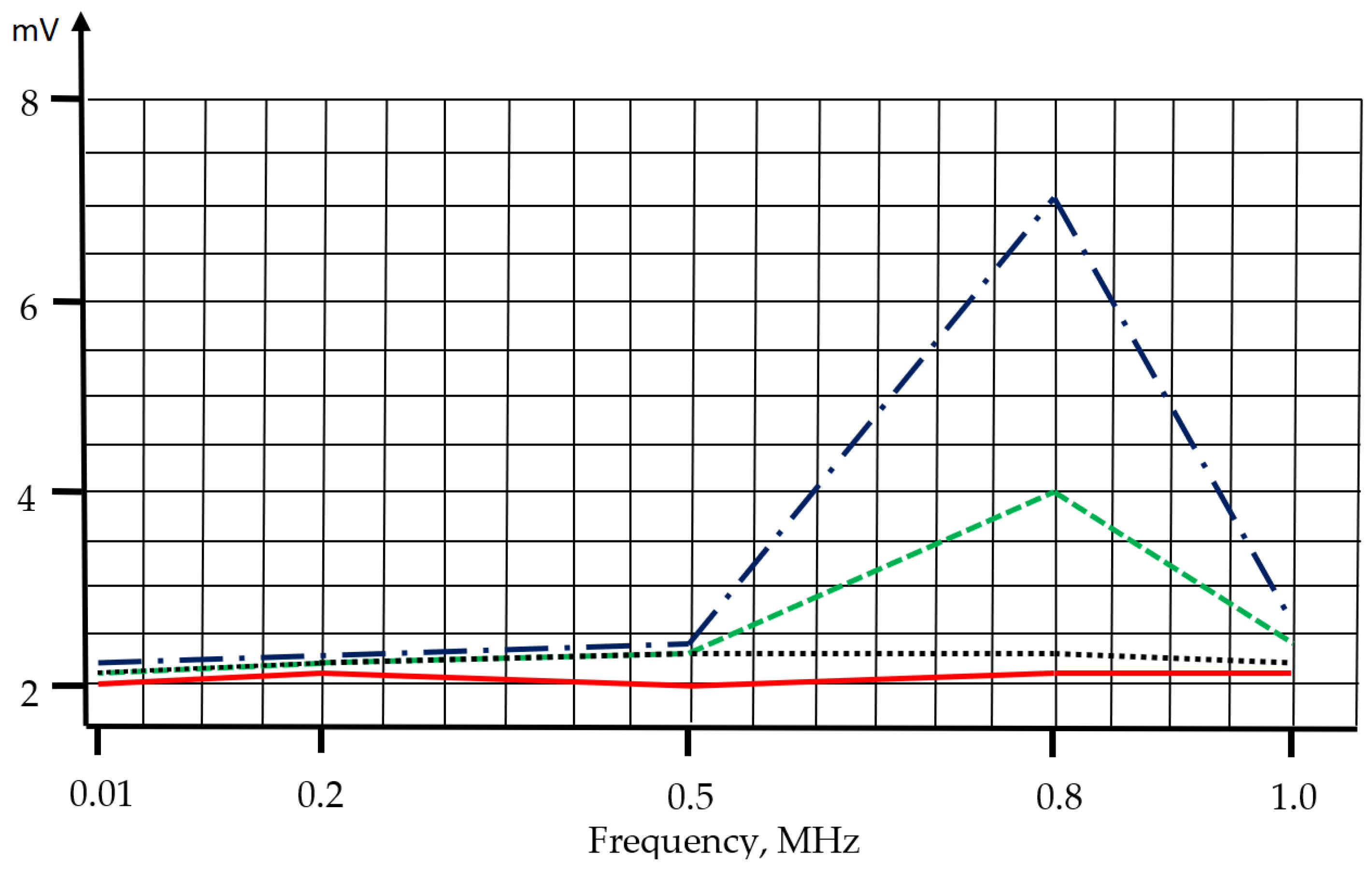
We used the abovementioned recommendations to develop a simplified model of the electrical conductivity sensor with four platinum electrodes placed inside a quartz glass tube with an inner diameter of 8 mm and a length of 60 mm; this tube was then placed in a sealed case and tested under high pressure. Like the SBE911 model described above that features a water pump, this sensor design is not perfect. The sensor model was also equipped with an impedance measurement module operating in situ at constant frequencies within the range of 0.01–1.0 MHz. The sensor model was tested during the marine trip together with the CTD and SVP devices. It produced additional data about suspended impurities in the seawater. The impedance sensor model helped us record suspended impurities corresponding to the impurities recorded by the ultrasonic SVP device and missing in the electric conductivity channel of the CTD probe. In this case, the operating frequency was about 0.8 MHz.

A simplified function diagram of the impedance measurement module together with the equivalent 4-electrode conductometric cell is shown above in Figure 2. The impedance measurement module consisted of the reference resistor Rref, from which the amplitude of a sinusoidal signal of a certain frequency was fed to the measuring unit. The impedance was determined by the equation Z_j = U4·Rref/(U3 − U4). The impedance measurement module operated at 5 constant frequencies—0.01, 0.2, 0.5, 0.8, and 1.0 MHz—with a homogenization duration of 1 s an each of them. The entire measurement cycle lasted for 5 s.

If we extend the functional capabilities of metering channels for electrical conductivity and sound speed of the CTD and SVP devices by using impedance and acoustic attenuation, we could obtain quantitative and qualitative parameters of suspended materials in seawater without using any additional tools.

The key measured parameters related to absolute salinity (S_A) and density (ρ) include relative electrical conductance (χ), sound speed in water (c), temperature (T), and hydrostatic pressure (P). To calculate absolute salinity and density using the parameters measured in situ, we used the following algorithms:

(1) S_A = S_A1(T, P, χ).

(2) S_A = S_A2(T, P, c).

(3) S_A = S_A3(T, P, ρ).

(4) ρ = ρ₁(T, P, c).

(5) ρ = ρ₂(T, P, S_A1).

(6) ρ = ρ₃(T, P, S_A2).

The connection between absolute salinity and practical salinity of seawater is set by the following relationship in TEOS-10 manual [11]:

$$S_A=\left(35.16504/35\right)S_P+\delta S_A\left(x,y,P\right),\hspace{0.17em}\mathrm{g}/\mathrm{kg}.$$

(7)

Here, δS_A(x, y, P), g/kg is the “absolute salinity anomaly”, which should consider the disturbances in the constancy of the salt composition of seawater. Thus, to the problems associated with finding reliable values of the practical salinity (S_P) of seawater (which is calculated by considering conductivity and should characterize the influence of the ionic component of the mass of dissolved substances), if the water passes through a 0.2 μm filter, there are added the problems of zoning of disturbances of the seawater salt composition constancy and definition estimates of the corresponding values of the anomaly of absolute salinity with reference to geographic coordinates (x, y) and depth (or pressure, P) with considering the presence of solid suspensions.

To calculate the density on the SVP device data, we used the equation of state [18]:

ρ = ρ (T, P, c).

(8)

To construct this equation, we used the international Equation of State of Seawater TEOS-10 [11]. The initial data array {ρ_m, c_m, T_m, P_m, S_Am}, m = 1, …, M was generated with using density and sound speed equations from the TEOS-10 system [11]. The couples of the value densities ρ (T_m, P_m, and S_Am) and sound speeds c (T_m, P_m, and S_Am) were calculated between melting curve and 40 °C, between 0 and 120 MPa of hydrostatic pressure, and between 0 and 42 g/kg of salinity. The ranges of changes in the speed of sound and density were approximately 1300–1800 m/s and 990–1090 kg/m³, respectively.

The seawater density interpolation Equation (8) has the following polynomial form:

$$\gamma ={\displaystyle \sum _{i=1}{\displaystyle \sum _{j=1}{\displaystyle \sum _{k=1}{b}_{ijk}{\tau }^i{\pi }^j{\omega }^k}}}$$

(9)

where γ = (ρ − ρ₀)/ρ*; τ = (T − T₀)/T*; π = (P_abs − P₀)/P*; ω = (c − c₀)/c*; ρ₀ = 990 kg/m³; ρ* = 100 kg/m³; T₀ = −10 °C; T* = 50 °C; P₀ = 0.101325 MPa; P* = 120 MPa; c₀ = 1300 m/s; and c* = 500 m/s.

Equation (9) explicitly expresses the functional dependency between the density of seawater and parameters T, P, and c and can be useful in marine research. The advantage of this equation is that salinity is not explicitly present in it, although, of course both the density and the sound speed of seawater are functionally related to its salinity. An equation like this helps to eliminate the indirect (via conductivity) salinity measurements by replacing them with direct sound speed measurements.

CTD and SVP probes are used for the synchronous in situ measurements of two different groups of seawater parameters (see

Table 3. The measured parameters of the CTD and SVP probes.

In Situ Measured Parameters	CTD	SVP
Temperature (T)	Yes	Yes
Hydrostatic pressure (P)	Yes	Yes
Relative electrical conductivity (χ)	Yes	No
Sound speed (c)	No	Yes

).

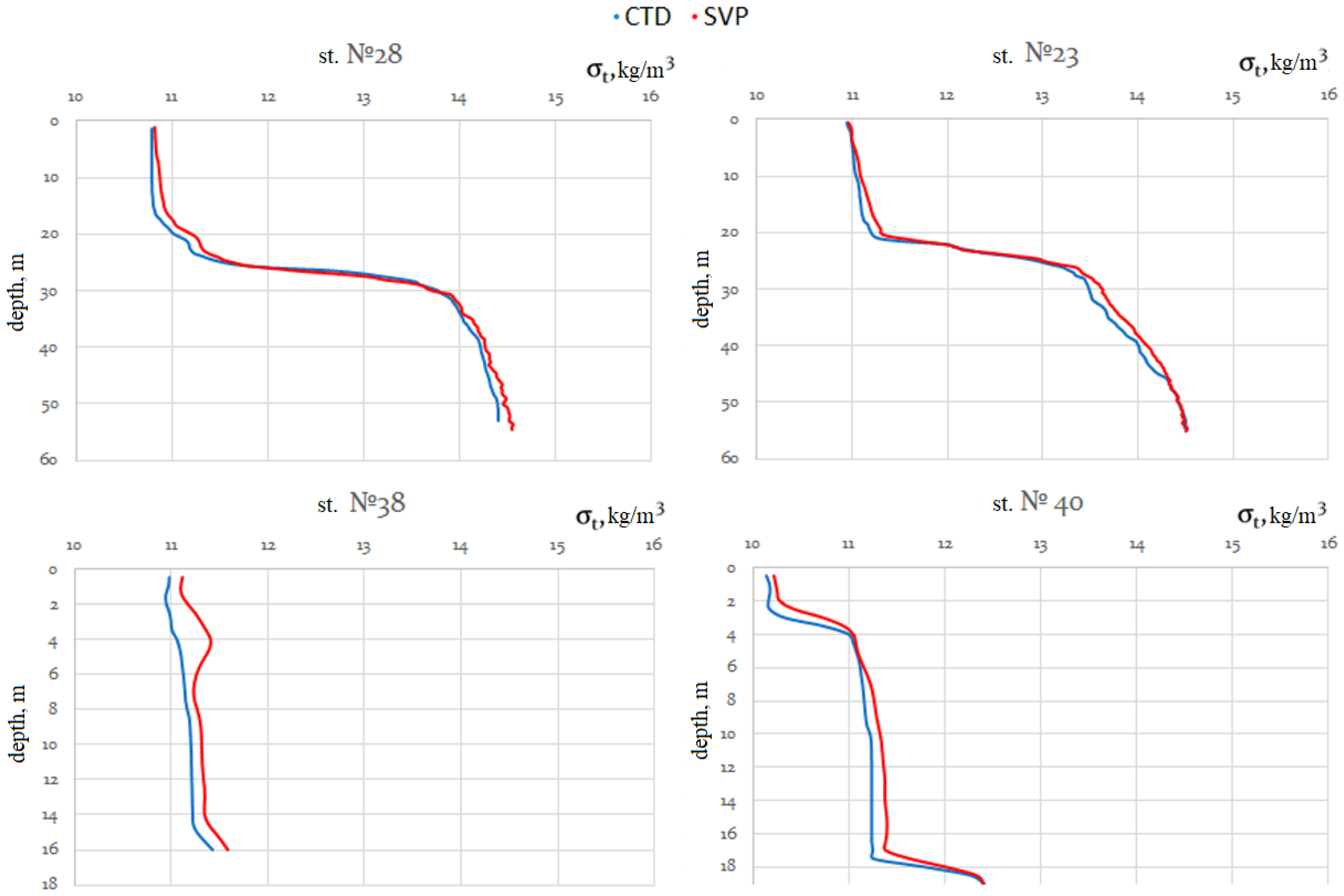
The two groups of parameters measured by the CTD and SVP probes can be further used to calculate of two usually different density values of seawater.

The differences in the density values obtained from CTD (ρ_CTD) and SVP (ρ_SVP) data are due to the fact that there are fundamental and significant differences between the physical processes of the passage of electric current and the propagation of sound in seawater. It should be noted that the value of the measured CTD relative electrical conductivity is only affected by the total ionic component of substances dissolved in seawater, i.e., only electrolyte solutions in seawater. At the same time, the speed of sound propagation measured by SVP is affected by the total mass fraction of all substances dissolved and suspended in seawater.

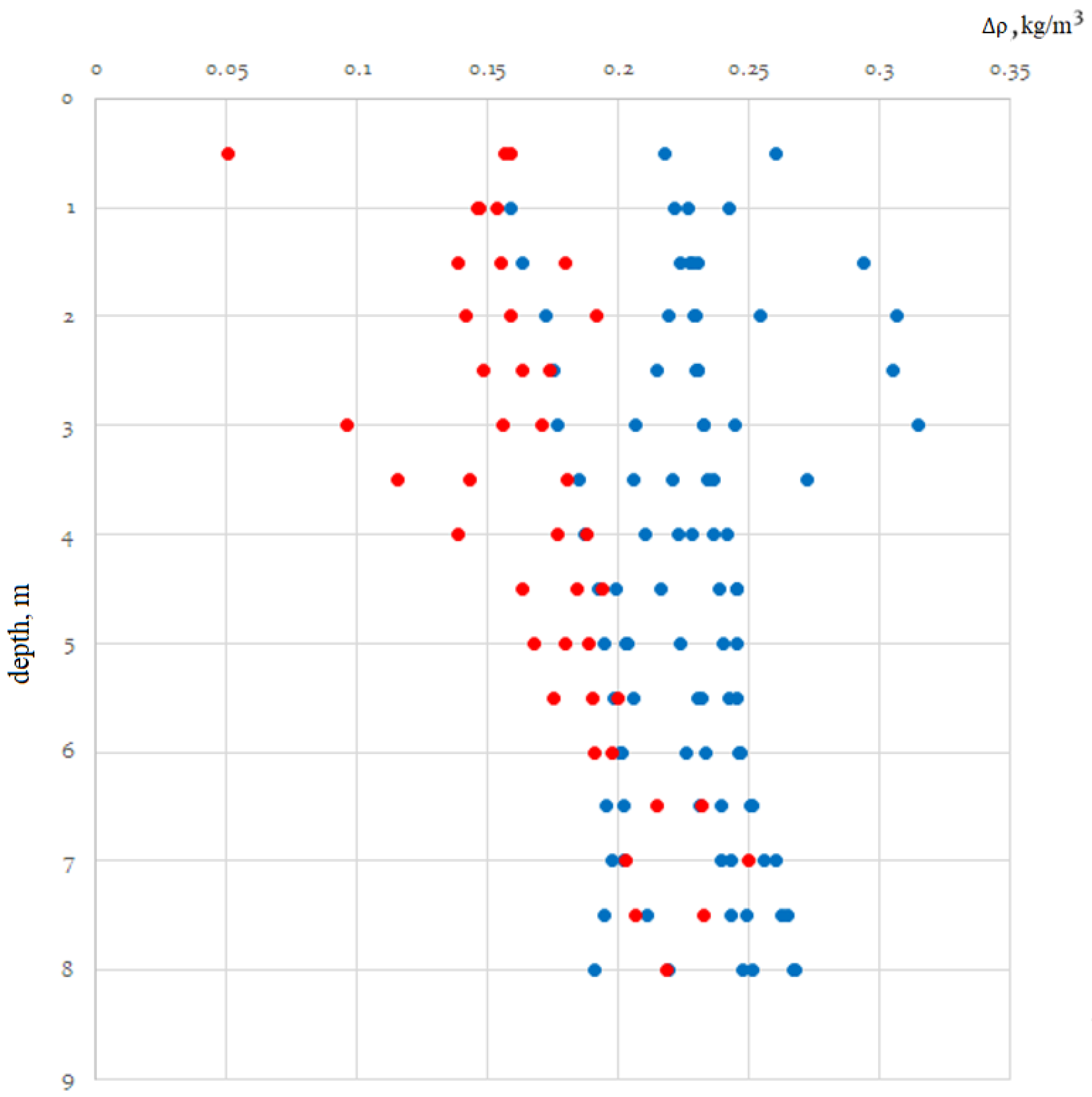
Therefore, the difference (delta) of densities can be used to estimate the amount of suspended matter in seawater:

∆ρ = ρ_SVP − ρ_CTD,

(10)

where

ρ_CTD = ρ (T, P, S_R),

(11)

S_R = (35.16504/35) S_P (T, P, χ)

ρ_SVP = ρ (T, P, c).

(12)

Here, S_P = S_P(T, P, χ); practical salinity is presented in the form of a special algorithm within the framework of the International Scale of Practical Salinity from 1978 [19,20].

The international Thermodynamic Equation Of state of Seawater TEOS-10 [11] and the authors’ equation [18] for calculating the density of seawater from measurements of the sound speed can be used, respectively, as equations for ρ_CTD (11) and ρ_SVP (12).

3. Results

Now, we analyze the results of measurements taken in the Black Sea and the Sea of Azov. The measurements were carried out in the period from 19 July 2017 to 24 July 2017 during the 96th expedition of Professor Vodyanitsky research vessel. The measurement results were not affected by the seasonal variability of the studied fields due to the short duration of the expedition. However, daily variability could have affected the results depending on the strength and direction of the wind, sea currents, and waves.

Based on the two described methods for determining the density of seawater, we calculated two profiles of the density anomaly (σ_t = ρ − 1000) depending on the depth (z) for each of the stations where measurements were made via vertical probing using the CTD and SVP instruments. Figure 3 and Figure 4 show the density anomaly profiles on the stations in the Black Sea and Sea of Azov, respectively.

These charts show that density anomaly profiles had similar shapes, but the density calculated using the equation ρ = ρ (T, P, c) exceeded the density calculated using the equation ρ = ρ (T, S_A, P) by ∆ρ = 0.20 kg/m³ on average.

4. A Differences Analysis of Density Profiles

Using the measurement data obtained with the CTD and SVP devices, we performed a difference analysis of vertical density profiles for the stations in the Black Sea and the Sea of Azov. For each of the stations, we found the difference (delta) of densities at various horizons by steps of 1 m. The density average delta for the Black Sea was 0.23 kg/m³, with a root-mean-square deviation of 0.05 kg/m³. The density average delta for the Sea of Azov was 0.16 kg/m³, with a root-mean-square deviation of 0.03 kg/m³. The distribution of density delta across the density horizons is shown in Figure 5. For the Black Sea, ∆ρ is marked in blue, and for the Sea of Azov, it is marked in red.

The study of measurement results obtained at various horizons (2, 4, 6, and 8 m) at Station 38 using the impedance measurement module confirmed the possibility of using this parameter for the detection of suspended impurities. Figure 6 shows impedance value charts for various constant frequencies at horizons of 2, 4, 6, and 8 m. From Figure 6, it follows that at horizons of 2, 6, and 8 m, impedance did not rapidly change at different frequencies. However, at a depth about 4 m and a frequency of 0.8 MHz, the signal amplitude harshly changed. The changes in the acoustic signal parameter at the same horizon of this station also confirmed the presence of suspended impurities in seawater.

5. Discussion

Following the analysis of the measurements and calculation results shown in Figure 3, Figure 4, Figure 5 and Figure 6, we came to the following conclusions.

• The main instrumental error of the devices was additive and equally contributed to the measurement results. The calculated density difference profiles characterized differences in the ionic composition of the Black Sea and Sea of Azov water.
• At some stations, deviations of the density difference from the average values up to ±0.1 kg/m³ were recorded. Such an increase in the density difference indicates the presence of suspended impurities, the effect of which on electrical conductivity is poorly understood and has not yet been taken into account in the calculations.
• At Station 38 (see Figure 3) in the Black Sea on the horizons of 3–4 m, the density values obtained through sound speed measurements by the SVP device were increased. At the same time, there were almost no changes in electric conductivity at the main operating frequency of the conductivity channel of the CTD probe. The difference analysis of density values showed an anomaly spot of ∆ρ reaching the maximum value of 0.31 kg/m³.
• At Station 44 in the Sea of Azov (see Figure 4), there was a drop in the density values measured through sound speed. We assume that this was caused by air bubbles, although the electrical conductivity channel did not find such impurities.
• The use of extra information produced by the acoustic attenuation and impedance metering channel models confirmed the presence of suspended impurities because the measured acoustic attenuation and impedance were directly related to the density and concentration of particles.

Figure 7 shows the vertical profiles of density differences between the measurements taken by the CTD and SVP probes sketched on the map of operations.

The results of the calculations were used to chart the density delta distribution fields for various horizons. Figure 8 shows the density field charted using the measurements taken by the CTD and SVP probes at a depth of 3 m.

The anomaly ∆ρ reached a maximum value of 0.31 kg/m³, as could be clearly seen in the gulf of Feodosia near Cape Chauda. This is an indirect sign of anthropogenic pollution in the area, which features an oil loading terminal and experiences regular problems with wastewater.

6. Conclusions

None of the existing methods provide a complete understanding of the distribution of density and salinity of seawater (especially in shelf zones) when it has various suspended impurities. Therefore, oceanological research must combine various instruments based on different physical principles to study the parameters of water. This work suggests improving mass-produced devices without adding new measuring channels and using improved processing methods for obtained data. This could significantly increase the reliability of measurements and reduce marine research costs.

The use of the suggested difference technique for processing the data obtained with the CTD and SVP devices can help assess the correctness of the interpretation of vertical profiles of density and salinity obtained with the CTD probe in a shelf zone. To do this, we need to develop new algorithms and models while taking the measurements obtained with the SVP into account.

The developed impedance and acoustic attenuation sensor models allow for the improvement of the functional capabilities of sound speed and water sensors without structural modification due to the improvement of hardware and software solutions, the improvement of the widely used CTD and SVP devices, and the retrieval of additional qualitative data on the type of suspended impurities in seawater.

7. Patents

RU2754107, ‘Method for Automatic Determination of Parameters of The State of Seawater in Ocean Conditions’. Authors: Aleksandr N. Grekov, Nikolay A. Grekov, Evgeniy N. Sychev.