Article

The Difference in Wave Dynamics between SARS-CoV-2 Pre-Omicron and Omicron Variant Waves

by
Franz Konstantin Fuss
1,*,
Yehuda Weizman
1,2 and
Adin Ming Tan
1,3
1
Chair of Biomechanics, Faculty of Engineering Science, University of Bayreuth, 95440 Bayreuth, Germany
2
Department of Health and Medical Science, School of Health Science, Swinburne University of Technology, Hawthorn, VIC 3122, Australia
3
Faculty of Health, Arts and Design, Swinburne University, Melbourne, VIC 3000, Australia
*
Author to whom correspondence should be addressed.
COVID 2023, 3(1), 28-50; https://doi.org/10.3390/covid3010002
Submission received: 16 November 2022 / Revised: 17 December 2022 / Accepted: 22 December 2022 / Published: 26 December 2022

Abstract

:
Compared to previous SARS-CoV-2 variants, the Omicron variant exhibited different epidemiological features. The purpose of this study was to assess the wave dynamics of pre-Omicron and Omicron waves in terms of differences and similarities. We investigated the COVID-19 waves since the beginning of the pandemic up to 28 August 2022, 1000 waves in total, as to their effectiveness for flattening the curve, calculated from the first and second time derivative of the daily case data. The average number of Omicron waves per month (42.78) was greater than the one of pre-Omicron waves per month (25.62). Omicron waves steepen and flatten the curve significantly faster, more effectively and with sharper peaks. Omicron waves generated more daily case data than pre-Omicron waves; the pre-Omicron trend showed increasing numbers over time, whereas the Omicron trend showed decreasing numbers. In denser populated countries, pre-Omicron waves were managed more effectively, in contrast to Omicron waves which were managed less effectively (but more effectively in less densely populated countries). This study provides the evidence for a different behaviour of Omicron waves in terms of wave dynamics, and thereby confirms that the Omicron variant is not only genetically different but even more so in terms of epidemiological dynamics.

1. Introduction

Since the beginning of the coronavirus disease (COVID-19) in late 2019, the severe acute respiratory syndrome coronavirus 2 (SARS-CoV-2) was affected by mutations, leading to new variants of the virus. Some of these variants were classified as variants of concern (VOC), such as Alpha, Beta, Gamma, Delta, and Omicron. VOC are characterised by increased human-to-human transmissibility [1].
The most recent variant, Omicron, emerged in Botswana and South Africa in November 2021, rapidly repressing the Delta variant. It was first reported to the WHO on 24 November 2021 [2,3], and on 26 November, the WHO classified the Omicron as a variant of concern [4].
Specifically, the Omicron variant showed slender and sharp spikes of excessive daily case data that surpassed by far any data of the preceding waves. These spikes rose almost as steeply as they fell. According to the CDC [5], “Omicron spreads more easily than earlier variants, including the Delta variant”, and “Omicron causes less severe illness and death in general”. The surge of Omicron cases since the end of 2021 seems to be due to the ability of the Omicron variant to evade antibodies generated by vaccination or past infection [6], as well as due to a shorter serial interval [7,8] and incubation period [9], and high transmission, specifically in household settings [10]. Another peculiarity of the clades of Omicron variant (12K/L & 22A/B/C/D; Figure 1) is that their genetic distance to the root clade is greater than any other of the SARS-CoV-2 clades (19-21H), based on a real-time tracking method of pathogen evolution [11].
These features of the Omicron variant waves suggest that the wave dynamics are different to the pre-Omicron waves. There is some literature on Omicron dynamics, such as: increased prevalence in January 2022 compared the two preceding months [4]; changes in the reproductive number relative to the deadline of the Shanghai lockdown [12]; and “lower peak viral RNA and a shorter clearance phase” compared to Delta infections [13]. To the best of the authors’ knowledge, there is no comprehensive study available in the literature, that deals with comparing the dynamics of pre-Omicron and Omicron waves.
The aim of this study is to identify and calculate wave parameters of all COVID-19 waves since the beginning of the pandemic and to compare the parameters of pre-Omicron and Omicron variant waves. The research question behind this aim reads as follows: are Omicron variant waves dynamically different from pre-Omicron variant waves?

2. Materials and Methods

2.1. Data of Daily Incidence

We used the daily updated dataset of daily incidence COVID-19 data provided by “Our World in Data” [14] up to 28 August 2022, downloaded from GitHub [15]. We analysed the data of 210 countries and dependencies (Appendix A), and excluded twenty (Appendix A), because of missing data (e.g., North Korea) or too few data (e.g., Vatican).

2.2. Data Processing

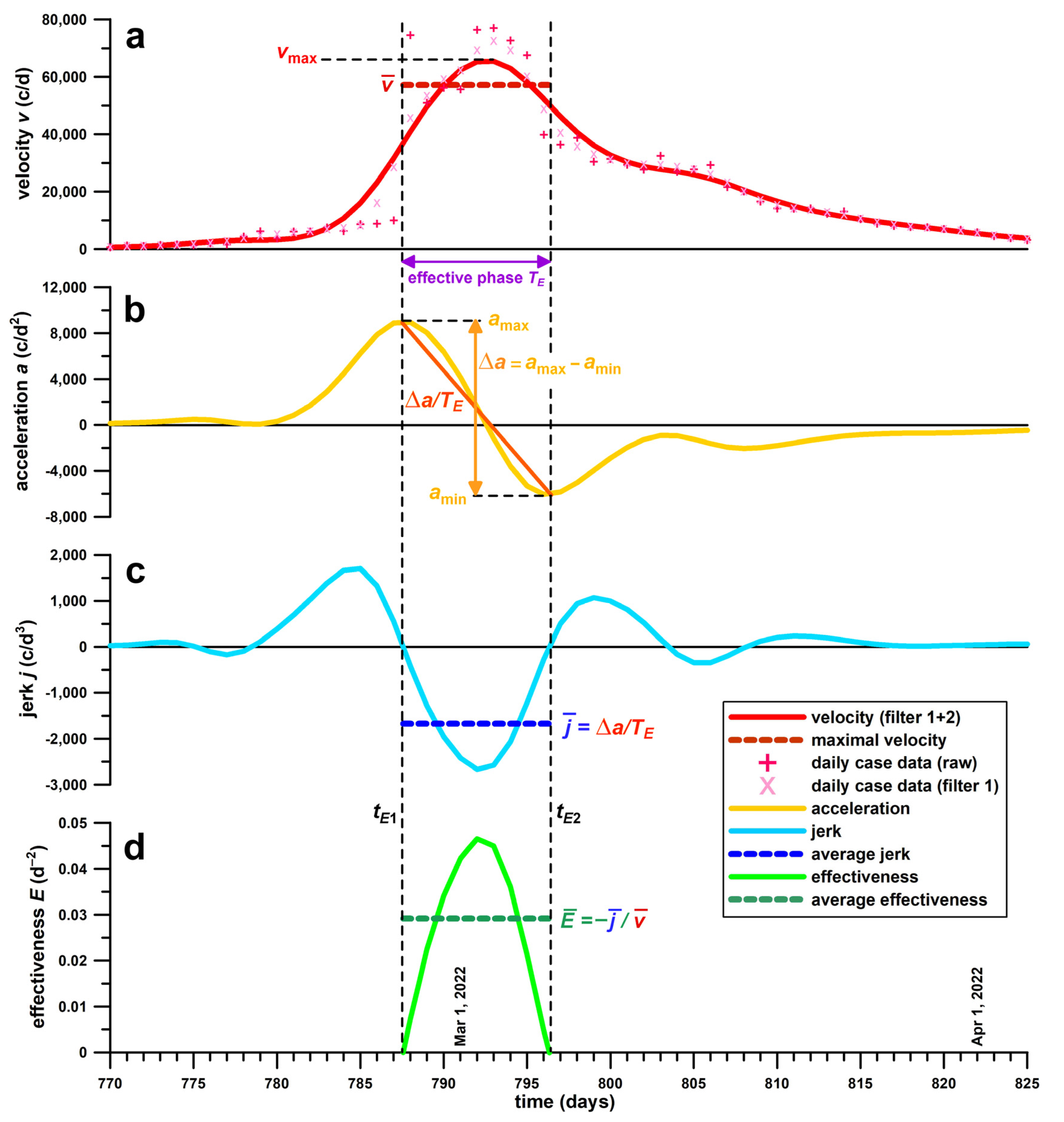
We used the method of Fuss et al. [16,17] for filtering the data and extracting the effectiveness parameters. The daily new case data were pre-filtered by subjecting them to a double running average filter (1st-order Savitzky–Golay filter) with a window width of 3 data (Figure 2a). The major data fit for identifying the trend was performed with a running quadratic filter (2nd-order Savitzky–Golay filter) over a window of 13 data (Figure 2a). The resulting dataset was denoted the velocity v (Figure 2a) of the spreading viral disease. Subsequently, we calculated the numerical time derivative of v twice, to obtain the acceleration a and the jerk j (Figure 2b,c). The major decrease of the acceleration (i.e., the major transition from acceleration to deceleration) is denoted by the effective phase or period, TE (measured in days, in this study as integers). The boundaries of TE correspond to the peak acceleration and deceleration (Figure 2b). Across TE, j is negative on average (Figure 2c). The effectiveness parameter, E, is the ratio of the average j to average v, both averaged across the TE (Figure 2d). The ratio ρ of E to TE is a further effectiveness parameter. Another ratio, ς, is defined as ς = C E−0.5 TE−1, where C is a constant [16].
In addition, we investigated the filtered daily case data at the peak of each wave (peak velocity vmax; Figure 2a), both the actual numbers as well as the peak case numbers normalised to the population of the respective country or dependency.
The effective reproduction number, Reff, was not included in this research, as Reff does not allow defining the TE [16,17]. Nevertheless, Reff is related to our effectiveness parameter E, as ER, the effectiveness calculated from Reff, corresponds to the average decrease of log(Reff) per unit time, across TE [16]. ER correlates well with E, with the regression slope also depending on logς [16].

2.3. Explanation and Definition of Effectiveness Parameters, and Their Practical Application in the Public Health Context

We define four effectiveness parameters [16,17], all of which address different aspects of the effectiveness of controlling the disease, also expressed as ‘flattening the curve’.
(1)
The effectiveness E, sensu stricto, refers to the rate of change of acceleration, that is, how quickly the positive acceleration peak, amax, becomes negative, amina/TE; Figure 1). As the gradient Δa/TE is case number dependent (velocity dependent), it has to be normalised to the average velocity during the effective phase TE. The greater E, the more effectively an epidemic wave is managed.
(2)
The duration of the effective phase, TE, refers to the interruption of the acceleration. Outside the effective phase, any control measures are ineffective, as the acceleration increases before the effective phase; and the deceleration decreases after the effective phase. A shorter effective phase TE, means that an epidemic wave is managed more effectively. This phenomenon can be explained easily from two waves with the same Δa, but different TE. Thus, the shorter TE, the greater is E.
(3)
The ratio ρ of E to TE addresses the following relationship: both E and TE are functions of the width of a wave [16]. The wider the wave in terms of daily case numbers, the smaller is E and the longer is TE. As E and TE are inversely related to each other, a greater E and a shorter TE result in a greater ratio ρ. The ratio ρ therefore combines the two individual effectiveness parameters of E and TE in a single one, referring to the magnitude of effectiveness E per unit time, i.e., per a single day. The greater ρ, the more effectively an epidemic wave is managed.
(4)
As mentioned before, both E and TE are functions of the width of a wave s [16], specifically in Gaussian wave profiles E = c1 s−2 and TE = c2 s, (where c1 and c2 are constants), and therefore the product of E and TE is proportional to a constant, namely: E·TEs−1. Any deviation from this constant indicates that the shape of the wave is no longer Gaussian. The ratio ς, mentioned above, and defined as ς = C E−0.5 TE−1, (where C is a constant [16]) addresses this problem. The shape factor logς defines the peak pattern of the velocity profile. If logς > 0, the velocity peak is triangular, if logς < 0, the peak is trapezoidal (with a plateau), and if logς = 0, the peak is round (Gaussian function). The greater logς > 0, the more triangular or pointed the velocity peak is, and the more effectively an epidemic wave is managed. A triangular shape indicates rapid change from increasing to declining daily case data, whereas a trapezoidal plateau shows that a wave is struggling with achieving a sustained decline of daily case data.
The practical application of the effectiveness parameters is that they gauge the effectiveness of control measures ‘intended’ for the effective management of waves. Retrospectively applied, the effectiveness parameters provide the coherence between cause (i.e., individual control measures) and effect (i.e., how effectively the curve was flattened). Since the beginning of the COVID-19 pandemic, countries and states have introduced different control measures, varying by type and severity, ranging from relaxed measures (e.g., Sweden) to severe lockdowns (e.g., Victoria). There is evidence that relaxed measures can be as effective, or as ineffective, as severe lockdowns [16]. In a previous study, we found no statistically significant difference between relaxed measures and lockdowns in terms of the effectiveness parameters [16]. These issues will be further addressed in the discussion section.

2.4. Wave Definition

In general, a ‘wave’ is usually referred to as a surge in new daily cases followed by a decline. According to Lipsitch, “there is no agreed definition for a second wave—it simply refers to a sustained upsurge in cases” [18]. Quoting Lipsitch [18], “A wave is just a metaphor. It is not a term with a precise definition in epidemiology…”. The same reference [18] also differentiates between a wave and a spike: “A spike [or upsurge] is a momentary phenomenon...”. Zhang et al. [19] offer two defining characteristics of a wave: (1) “some upward and/or downward periods”; (2) “the increase in an upward period or the decrease in a downward period have to be substantial by sustaining over a period of time to distinguish them from” a spike. Based on these characteristics, Zhang et al. [19] suggest the effective reproduction number Reff for defining an upward or downward period if Reff is greater or smaller than 1, respectively, for a sustained period, e.g., for the past 14 days.
In contrast to this suggestion, we define a wave based on the effective phase TE (Figure 2), the duration of which cannot be derived from Reff [16,17]. TE must be at least 5 days to constitute a wave. In addition to this, as a wave does not necessarily start, or end, with zero cases, we consider the amount by which a wave declines or increases, with respect to the preceding data. A wave must decline to at least half its peak value (peak velocity vmax, filtered data), or increase to at least twice the minimum value at the end of the preceding wave. If these conditions are not fulfilled, then two consecutive peaks are counted as a single wave.

2.5. Statistics

For statistical purposes, the effectiveness parameters TE, E, and ρ were log-transformed; whereas the shape parameter logς is already log-transformed. Note that for non-parametric tests, the rank of the median is the same in the original and log-transformed datasets.

2.5.1. Correlations

The correlation analyses served for comparing the slopes for pre-Omicron and Omicron waves, when correlating log E to log TE, and log ρ to logς. The null hypothesis was that slopes for pre-Omicron and Omicron waves were equal.

2.5.2. Regressions

The regression analyses served for establishing the trend of wave effectiveness parameters (log TE, log E, log ρ, logς) over time., that is, the course of the epidemic. As the trends can be increasing or decreasing data with time, the null hypotheses and alternative hypotheses are as follows:
-
apparently increasing trend:
-
H0: the effect (gradient of the trend) is smaller than or equal to zero
-
H1: the effect is greater than zero
-
apparently decreasing trend:
-
H0: the effect is greater than or equal to zero
-
H1: the effect is smaller than zero
As these tests cannot distinguish between zero and an effect in a particular direction, these tests are one-sided. Accordingly, the one-sided p-value was calculated for rejecting (p < 0.05), or failing to reject, the null hypothesis.
As far as the normality of the datasets is concerned, the data were log-transformed in the first place, and according to the central limit theorem, as sample sizes increase from moderate to large sizes, the normality assumption for the residuals is no longer required.

2.5.3. Comparison of Pre-Omicron and Omicron Wave Data

We compared the data of pre-Omicron and Omicron waves with the Mann–Whitney U test. A significant difference between the two medians (pre-Omicron and Omicron) was established from the two-tailed p-value. The effect size, r, was calculated from r = 1 − 2U1/(U1 + U2), where U1 < U2. The effect was interpreted according to McGrath and Meyer [20].

2.5.4. Influence of Geographic and Socioeconomic Data

We considered the following datasets: population P of a country or dependency [21]; land area A [22]; gross domestic product (GDP) [23]; and educational index I [24]. We normalised the GDP to P, to obtain the GDP per capita G; and P to A to derive the population density D. All five parameters, P, A, G, I and D, were log-transformed. These parameters were associated with each country of the wave effectiveness parameter dataset.
For establishing a relationship between wave effectiveness parameters and geographic and socioeconomic data, we divided, for example, the land area A dataset into two unequal size subsamples, and compared the medians of the wave effectiveness parameters (e.g., effectiveness E) within each subsample regarding significant differences. This method is an analogy to the Median–Median Line method by Wald [25], who divided a dataset into two equal size subsamples, separated by the median of the independent parameter. This method was optimised by Fuss et al. [26] with a floating separation line, the optimum position of which was found at the maximum separation of the medians (minimum p-value) on either side of the separation line. A similar approach was used by Fuss et al. [16] for exactly the same purpose as intended in this study. However, we optimised the method further by seeking the optimal separation line within the central 40% percentile (i.e., between 30th and 70th percentile), in contrast to the central 60% percentile used by Fuss et al. [26], based on the minimum p-value of a t-test. The t-test served for comparing the medians of, e.g., E of large and small area countries. An F-test (one-sided p-value) determined whether an equal-variance or unequal-variance t-test had to be performed. Another criterion was the continuous trend condition throughout the central 40% percentile of data, e.g., E of large area countries is consistently smaller than E of small area countries, whereby the terms smaller (or greater/larger) refer to a significant difference between the two medians of E (e.g., one median for large area countries, and another one for small area countries). This approach excludes bidirectional trends (subsequent sections within the same median of greater, insignificantly different, or smaller data) which are considered inconclusive. Once the optimal separation line was identified, then the two cohorts, e.g., E-medians of large/small area countries were compared with the Mann–Whitney U test to find the actual p-value at the separation point.
The ‘running line’ method is exemplified in Figure 3. Figure 3a shows the Box and Whisker plot of log A, where the box denotes the central 50% percentile. Figure 3b identifies the boundary values of log A, associated with the 30th and 70th percentile (central 40% percentile) of log A. Figure 3c shows the p-values associated with each line of separation, dividing the land area into large and small countries. Figure 3d zooms into the central 40% percentile for better visibility of the minimum p-value. Figure 3e shows the medians of log ρ of small and large area countries at any separation line, as well as the difference of the medians. Figure 3f zooms into the central 40% percentile and exhibits a continuous trend, that the median of log ρ of small area countries is significantly greater than the median of log ρ of large area countries.

3. Results

3.1. Wave Data

Since the beginning of the COVID-19 pandemic up to 28 August 2022, there were 1000 waves in 210 countries and dependencies, on average 4.76 ± 1.67 waves per country (1–9 waves). 615 of these waves were pre-Omicron ones, and 385 Omicron waves (ratio of 8:5).
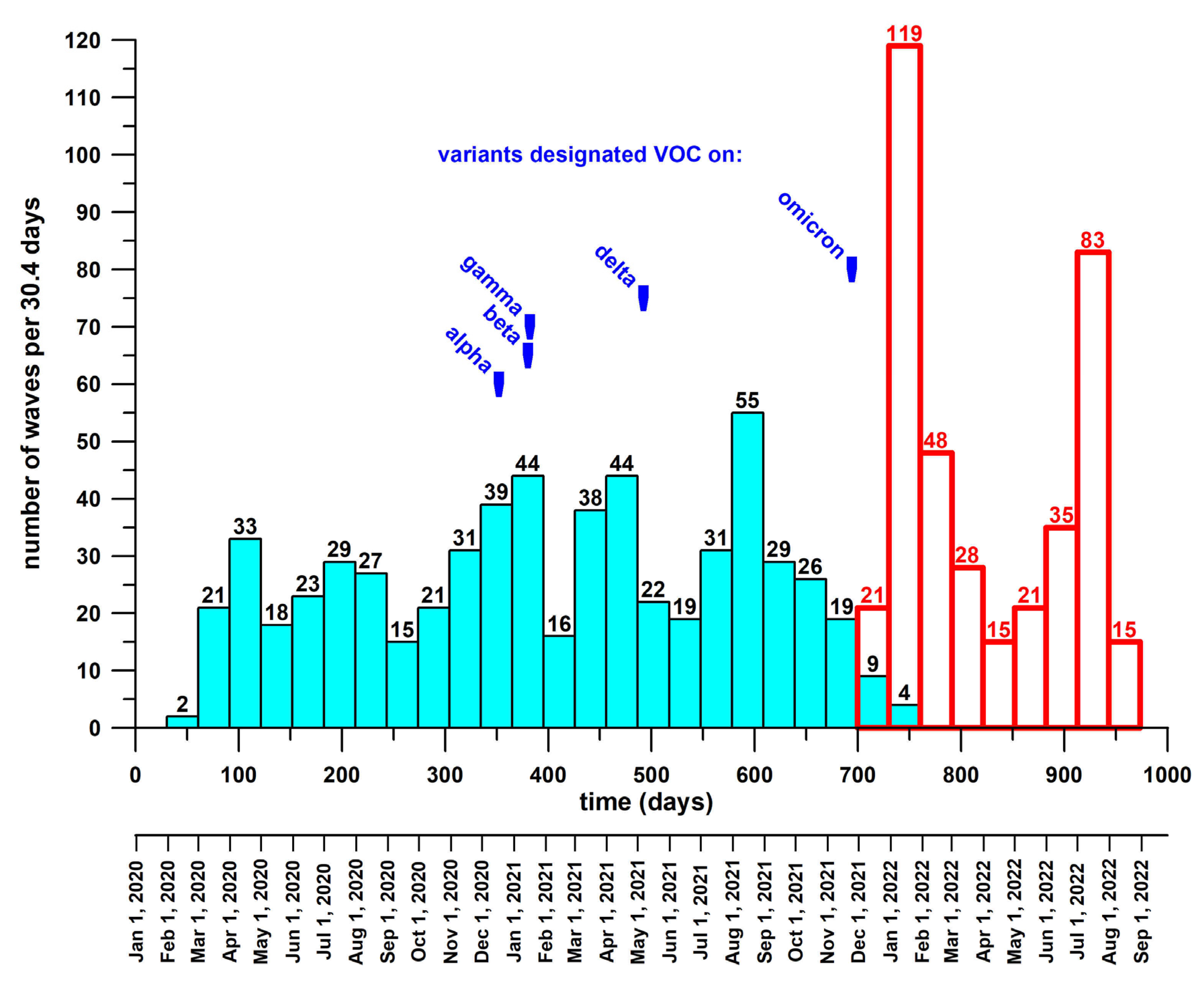
The wave histogram (Figure 4) shows that the peak number of Omicron waves was 119 in January 2022, followed by 83 waves in July 2022; whereas the peak number of pre-Omicron waves was at its maximum of 55 waves in August 2021. The wave distribution was, on average, 25.62 pre-Omicron waves per month and 42.78 Omicron waves per month.

3.2. Correlation Analysis of Effectiveness Parameters

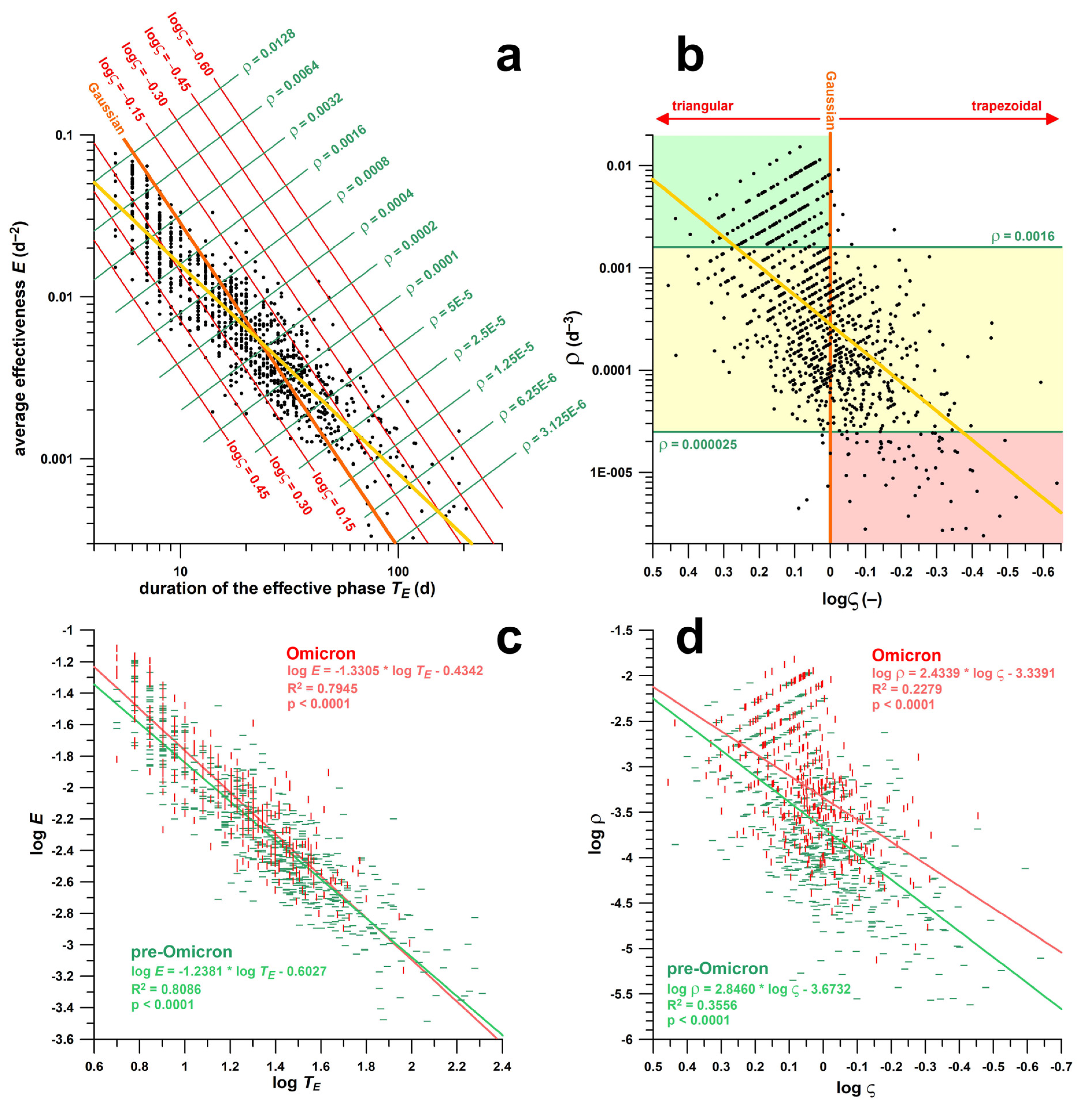
Figure 5a shows the correlation of the effectiveness E vs. the duration of the effective phase, TE, exemplifying that waves managed more effectively (shorter TE, greater E and ρ; independent of the control measures, if any) are more triangularly shaped (log ς > 0). This effect is further enhanced in Figure 5b where log ρ is correlated with log ς. Figure 5b is divided into three zones [16]: the green zone in the top left corner is almost exclusively populated with highly effective and triangularly shaped waves; the red zone in the bottom right corner is almost exclusively populated with less effective and trapezoidally shaped waves; the yellow zone in the centre, featuring waves of average effectiveness, is filled with waves of any shape pattern during the effective phase, from triangular over Gaussian (rounded) to trapezoidal.
The gradients of the correlations (pre-Omicron and Omicron waves) shown in Figure 5c, log E vs. log TE, are significantly different (p = 0.0291), whereas the gradients in Figure 5d, log ρ vs. log ς are not (p = 0.1362). The regression gradient of Omicron waves in Figure 5c is steeper than in pre-Omicron waves, which is due to less ineffective waves. The gradient of Omicron waves in Figure 5d, appears to be flatter than in pre-Omicron waves, equally due to less ineffective waves and less triangular wave shapes. This difference, however, is not significant because of more data spread as seen from the low R2.

3.3. Regression Analysis of Effectiveness Parameters and Peak Daily Case Data against Time

3.3.1. Data of All Waves

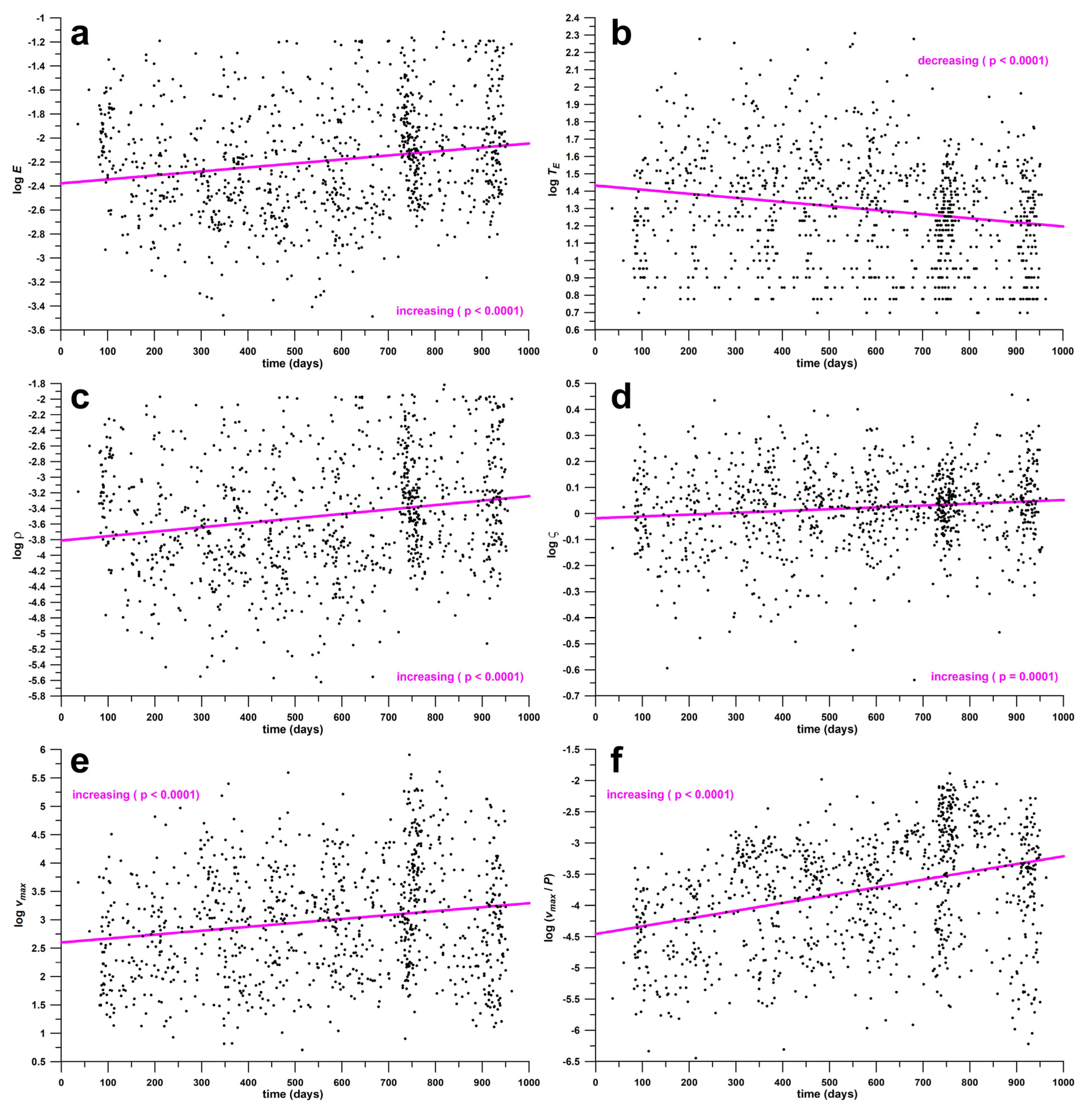
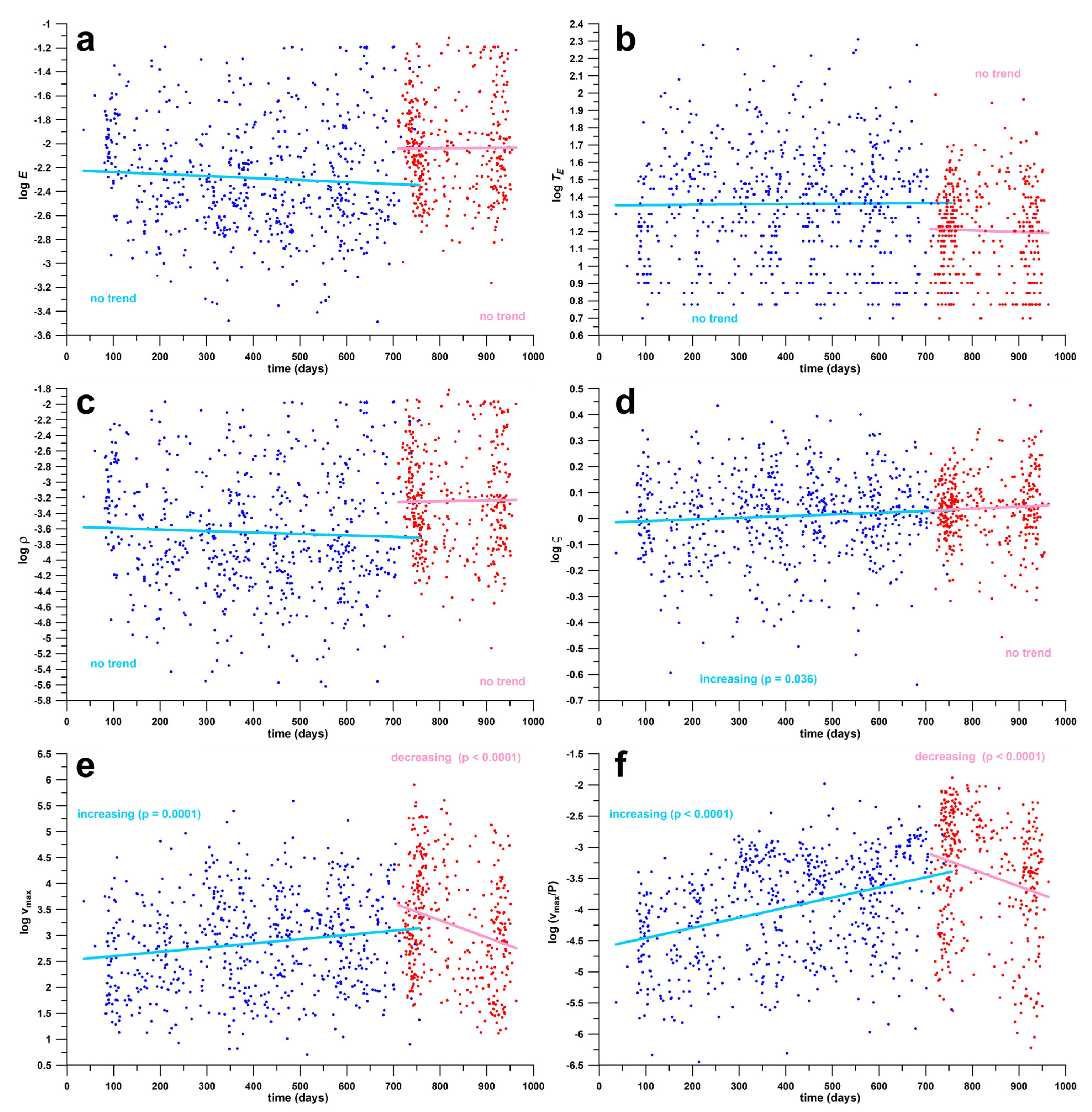
The trends of all parameters, log TE, log E, log ρ, log ς, log vmax, and log (vmax/population), were significant (p ≤ 0.0001; Table 1, Figure 6). All but one parameter increased as the time does; log TE decreased. Thus, the preventive measures (relaxed, restrictions or lockdown) became more effective over time; the shape of the waves became more triangular; and the peak number of daily case data (filtered) increased over time (despite greater effectiveness).

3.3.2. Pre-Omicron and Omicron Waves Separated

There were no significant trends detected in effectiveness parameters (log TE, log E, log ρ; Table 1, Figure 7). The shape factor, logς, increased (p = 0.036) over time in the pre-Omicron waves. The apparent increase of logς in the Omicron waves was not significant (p = 0.18). The peak number of daily case data (filtered), log vmax, and log (vmax/population), increased over time in the pre-Omicron waves (p < 0.0001), but decreased in the Omicron waves (p < 0.0001).

3.4. Comparison of Pre-Omicron and Omicron Data

Why did the effectiveness parameters show a significant trend across all waves, while the waves separated in pre-Omicron and Omicron did not show any significant trend? Comparing the medians of parameters for pre-Omicron and Omicron waves provided an answer (Table 2). Figure 8 shows the box-plots of the effectiveness parameters. Table 2 shows the results of the Mann–Whitney U test, including medians, p-values and effect sizes.
From Table 2 and Figure 8, the preventive measures (relaxed, restrictions or lockdown) are significantly more effective during the Omicron waves; the shape of the Omicron waves became significantly more triangular; and the peak number of daily case data (filtered) significantly increased during the Omicron waves (despite greater effectiveness). The effect size r (Table 2) and the associated effect mirror the closeness of the two medians relative to the pooled dispersion of the data. In the shape factor, logς, the medians are relatively close such that the two medians exhibit a Gaussian profile. In the peak number of daily case data (filtered) per unit population, log (vmax/population), the medians are relatively far apart, accounting for medians of 1.43 and 5.90 cases per ten thousand people, for pre-Omicron and Omicron waves, respectively, that is, four times as much. Note that the rank of the medians remains the same for original and log-transformed data.
The significant differences in medians between pre-Omicron and Omicron waves explains the significant trends shown in Figure 6. These trends are solely due to the different epidemiological dynamics between pre-Omicron and Omicron waves, and are, moreover, not mirrored in the individual wave trends of the effectiveness parameters (log TE, log E, logρ), that are not significant.

3.5. Relationship of Epidemiological Parameters with Geographical and Socioeconomic Data

To understand the epidemiological dynamics, the relationship within and across geographical and socioeconomic data has to be established. The geographical data, population (P) and land area (A), are related to each other (log P vs. log A, R2 = 0.6847); and so are the socioeconomic data, GDP per capita (G) and the educational index (I; log I vs. log G, R2 = 0.7137). There is a slight dependency between P and G (R2 = 0.0660, p < 0.0001), and P and I (R2 = 0.0084, p = 0.0028), in the sense that more populous countries are inhabited by richer and more educated people. The same slight relationship is true for A and G (R2 = 0.0749, p < 0.0001), and A and I (R2 = 0.0134, p = 0.0003), in the sense that larger countries are inhabited by richer and more educated people. Another slight relationship exists between D and G (R2 = 0.0163, p = 0.0001), and D and I (R2 = 0.0054, p = 0.0131): denser populated countries are inhabited by richer and more educated people.

3.5.1. Data of All Waves

The relationship between epidemiological parameters and geographical and socioeconomic data of all waves is shown in Table 3.
From Table 3, in more populous or larger countries, the preventive measures (relaxed, restrictions or lockdown) are significantly less effective (greater log E and logρ, and shorter log TE); the shape of the waves is slightly but significantly more trapezoidal; but the peak number of the normalised daily cases (filtered) is significantly smaller, which does not reflect the lower effectiveness.
In countries with richer and more educated inhabitants, the preventive measures (relaxed, restrictions or lockdown) are equally significantly less effective; the shape of the waves is slightly but significantly more triangular; and the peak number of the normalised daily cases (filtered) is significantly greater, as expected from lower effectiveness.
More densely populated countries show the same trends as countries with richer and more educated inhabitants do (D is positively correlated to G and I), except for log TE and log ς, which are insignificant.

3.5.2. Pre-Omicron Wave Data

The relationship between epidemiological parameters and geographical and socioeconomic data of pre-Omicron waves is shown in Table 4.
For P, A, G, and I, the results shown in Table 3 (all wave data) are matched in Table 4 (pre-Omicron wave data). The only difference is that logς was not affected by P, A, G, and I (insignificant results); and log TE was not affected by G.
In contrast to Table 3, in more densely populated countries, the preventive measures (relaxed, restrictions or lockdown) are significantly more effective.

3.5.3. Omicron Wave Data

The relationship between epidemiological parameters and geographical and socioeconomic data of Omicron waves is shown in Table 5.
For P, A, G, I and D, the results shown in Table 3 (all wave data) are matched in Table 5 (Omicron wave data). The only difference is that log TE and logς were not affected by A (insignificant results); and that log TE was significantly longer in more densely populated countries.
There were no differences between pre-Omicron and Omicron waves, except for the density D: in more densely populated countries, the preventive measures (relaxed, restrictions or lockdown) were significantly more effective (log TE, log E, logρ) in the pre-Omicron waves, and significantly less effective (log TE, log E, logρ) in the Omicron waves as well as in the all-wave cohort (only log E and logρ). The reason for this is that Omicron waves have greater medians of log E and logρ than the pre-Omicron waves, which overrides the pre-Omicron medians and produces in the all-wave cohort similar results as in the Omicron waves. In contrast to this, Omicron waves have smaller medians of log TE than the pre-Omicron waves, which does not suffice to mirror the pre-Omicron result in the all-wave cohort, that does not show a significant difference between the medians of log TE.

4. Discussion

The research question of whether Omicron waves are dynamically different from pre-Omicron waves can be answered clearly by pointing out the differences:
(1)
the average number of Omicron waves per month (42.78) was greater than the one of pre-Omicron waves per month (25.62) (Figure 4);
(2)
Omicron waves steepen and flatten the curve (cumulative data) significantly faster (shorter TE) and more effectively (greater E and ρ), and with sharper peaks (greater logς) (Table 2; Figure 5 and Figure 8);
(3)
Omicron waves generated more cases (vmax and vmax/P) than pre-Omicron waves; the pre-Omicron trend showed increasing numbers over time, whereas the Omicron trend showed decreasing numbers (Figure 7e,f);
(4)
in denser populated countries, pre-Omicron waves are managed more effectively (including shorter TE), in contrast to Omicron waves which were managed less effectively (including longer TE; Table 4 and Table 5).
Similar results, shared by pre-Omicron and Omicron waves, were: in more populous and larger countries, as well as in countries with richer and more educated citizens: waves are managed less effectively. The same trend was also seen in 92 countries (states, provinces, dependencies) during the 1st COVID-19 wave [16]. In this previous study, the population density did not have any influence on the effectiveness (as land area and population positively correlate with each other). However, in this present study, the population density did influence the effectiveness, with opposite trends for pre-Omicron and Omicron waves. It seems logical that waves are less effectively managed in denser populated countries (even if the previous study [16] did not show any evidence). In contrast to the Omicron waves, in the pre-Omicron ones the control measures were more effective in denser populated countries.
The terms velocity and acceleration used in this study should not be confused with similar terminology applied to the ratios of Farr’s [27] law by Pacheco-Barrios et al. [28]. Farr [27] defined ratios of subsequent data of a time series, with the data corresponding to the number of new cases or deaths within a time duration, such as the daily new cases or the velocity v used in our study. E.g., R1 = vt/vt+1 (where t denotes a time stamp), and R2 = R1(t)/R1(t+1). Farr [27] noticed that R2 ratios are very constant, mathematically indicating that the incident data follow a Gaussian function. When applying logarithm to a Gaussian function (velocity v), then we obtain a 2nd-order function, the first derivative (D1) of which is a 1st-order function, and the 2nd derivative (D2) is a constant. Pacheco-Barrios et al. [28] misinterpreted the ratio R1 as the velocity, and R2 as the acceleration of the epidemic. However, when relating R1 and R2 to D1 and D2, respectively, then R1 = e−D1 and R2 = eD2. R1 as a velocity ratio cannot be a velocity per se, as a ratio is unitless; and D1 is the time derivative of the logarithm of the velocity. Interestingly, as D1 equals the logarithmic growth rate K, the effective reproduction number Reff, based on the exponential equation given by Diekmann et al. [29] and the serial interval SI, is calculated from Reff = eD1 SI, which yields Reff = R1−SI.
The actual velocity and acceleration of a spreading contagious disease are subsequently put into context. When introducing control measures, independent of their severity, it is the cumulative case curve that should be flattened, which is the summation of the daily case data (velocity v). The rate of change of the acceleration a, in turn, is directly related to the effectiveness E (which corresponds to the 3rd time derivative of the cumulative case curve). The coherence between cause (i.e., individual control measures) and effect (i.e., how effectively the curve was flattened), depends on several factors:
(1)
The type of control measure; if there were no further influences, then the control measure is expected to succeed, and the effectiveness would correlate with the severity and complexity of the control measures, resulting in maximum coherence.
(2)
The compliance of the citizens [30], which can be enforced by restrictions but suffers when disagreeing with enforcement.
(3)
Socioeconomic status: citizens of richer countries are better educated and thus less likely to follow orders [16].
(4)
Geographical factors: smaller countries with less population manage the waves more efficiently, specifically small islands [16].
(5)
Timely introduction of control measures: if, e.g., a lockdown is introduced one serial interval before the end of the effective phase, then it was implemented too late and cannot contribute to the flattening of the curve anymore [17] which at this point is already completed.
(6)
Epidemiological factors, related to microorganisms (e.g., contagiousness), herd immunity, vaccines, etc.
Combining all these factors can result in zero coherence between control measure and effectiveness [16]. However, retrospectively seen, the effectiveness provides information about the combined effect of all the factors involved, and ultimately how effectively a wave was managed. In the case of the Omicron waves, their significantly greater effectiveness of wave management, compared to pre-Omicron waves, is unclear, specifically when considering the odds against high effectiveness, based on features mentioned in the discussion: Omicron spreads more easily [5] with a high transmission [10], evades antibodies generated by vaccination or past infection [6], and has a shorter serial interval [7,8] and incubation period [9]. These features, however, explain only the steep rise of daily case numbers, but neither their equally steep decline nor the effective management. Yet, there is another likely explanation, which is that the shockingly high daily case numbers forced citizens to be more compliant, which subsequently triggered the precipitous drop in daily cases.

Author Contributions

All authors contributed equally to the conceptualization, methodology, validation, investigation, formal analysis, resources, writing—original draft preparation, writing—review and editing, visualization and project administration. All authors have read and agreed to the published version of the manuscript.

Funding

This research received no external funding.

Institutional Review Board Statement

Not applicable.

Informed Consent Statement

Not applicable.

Data Availability Statement

The data presented in this study are available on request from any qualified researcher to the corresponding author.

Conflicts of Interest

The authors declare no conflict of interest.

Appendix A

Countries included in this study:
Afghanistan, Albania, Algeria, Andorra, Angola, Antigua and Barbuda, Argentina, Armenia, Aruba, Australia, Austria, Azerbaijan, Bahamas, Bahrain, Bangladesh, Barbados, Belarus, Belgium, Belize, Benin, Bermuda, Bhutan, Bolivia, Bonaire Sint Eustatius and Saba, Bosnia and Herzegovina, Botswana, Brazil, British Virgin Islands, Brunei, Bulgaria, Burkina Faso, Burundi, Cambodia, Cameroon, Canada, Cape Verde, Cayman Islands, Central African Republic, Chad, Chile, China, Colombia, Comoros, Congo, Cook Islands, Costa Rica, Cote d’Ivoire, Croatia, Cuba, Curacao, Cyprus, Czechia, Democratic Republic of Congo, Denmark, Djibouti, Dominica, Dominican Republic, Ecuador, Egypt, El Salvador, Equatorial Guinea, Eritrea, Estonia, Eswatini, Ethiopia, Faeroe Islands, Fiji, Finland, France, French Polynesia, Gabon, Gambia, Georgia, Germany, Ghana, Gibraltar, Greece, Greenland, Grenada, Guatemala, Guinea, Guinea-Bissau, Guyana, Haiti, Honduras, Hong Kong, Hungary, Iceland, India, Indonesia, Iran, Iraq, Ireland, Isle of Man, Israel, Italy, Jamaica, Japan, Jordan, Kazakhstan, Kenya, Kiribati, Kosovo, Kuwait, Kyrgyzstan, Laos, Latvia, Lebanon, Lesotho, Liberia, Libya, Liechtenstein, Lithuania, Luxembourg, Macao, Madagascar, Malawi, Malaysia, Maldives, Mali, Malta, Mauritania, Mauritius, Mexico, Micronesia (country), Moldova, Monaco, Mongolia, Montenegro, Montserrat, Morocco, Mozambique, Myanmar, Namibia, Nepal, Netherlands, New Caledonia, New Zealand, Nicaragua, Niger, Nigeria, North Macedonia, Norway, Oman, Pakistan, Palau, Palestine, Panama, Papua New Guinea, Paraguay, Peru, Philippines, Poland, Portugal, Qatar, Romania, Russia, Rwanda, Saint Kitts and Nevis, Saint Lucia, Saint Pierre and Miquelon, Saint Vincent and the Grenadines, Samoa, San Marino, Sao Tome and Principe, Saudi Arabia, Senegal, Serbia, Seychelles, Sierra Leone, Singapore, Slovakia, Slovenia, Solomon Islands, Somalia, South Africa, South Korea, South Sudan, Spain, Sri Lanka, Sudan, Suriname, Sweden, Switzerland, Syria, Taiwan, Tajikistan, Tanzania, Thailand, Timor, Togo, Tonga, Trinidad and Tobago, Tunisia, Turkey, Turks and Caicos Islands, Uganda, Ukraine, United Arab Emirates, United Kingdom, United States, Uruguay, Uzbekistan, Vanuatu, Venezuela, Vietnam, Wallis and Futuna, Yemen, Zambia, Zimbabwe.
Countries excluded from this study:
Anguilla, Falkland Islands, Guam, Guernsey, Jersey, Marshall Islands, Nauru, Niue, North Korea, Northern Cyprus, Northern Mariana Islands, Pitcairn, Puerto Rico, Saint Helena, Sint Maarten (Dutch part), Tokelau, Turkmenistan, Tuvalu, United States Virgin Islands, Vatican.

References

  1. Shahhosseini, N.; Babuadze, G.; Wong, G.; Kobinger, G.P. Mutation Signatures and In Silico Docking of Novel SARS-CoV-2 Variants of Concern. Microorganisms 2021, 9, 926. [Google Scholar] [CrossRef] [PubMed]
  2. Quarleri, J.; Galvan, V.; Delpino, M.V. Omicron variant of the SARS-CoV-2: A quest to define the consequences of its high mutational load. GeroScience 2022, 44, 53–56. [Google Scholar] [CrossRef] [PubMed]
  3. Gowrisankar, A.; Priyanka, T.M.; Banerjee, S. Omicron: A mysterious variant of concern. Eur. Phys. J. Plus 2022, 137, 100. [Google Scholar] [CrossRef] [PubMed]
  4. Elliott, P.; Eales, O.; Bodinier, B.; Tang, D.; Wang, H.; Jonnerby, J.; Haw, D.; Elliott, J.; Whitaker, M.; Walters, C.E.; et al. Dynamics of a national Omicron SARS-CoV-2 epidemic during January 2022 in England. Nat. Commun. 2022, 13, 4500. [Google Scholar] [CrossRef] [PubMed]
  5. Centers for Disease Control and Prevention (CDC). Variants of the Virus. Available online: https://www.cdc.gov/coronavirus/2019-ncov/variants/index.html (accessed on 15 October 2022).
  6. Willyard, C. What the Omicron wave is revealing about human immunity. Nature 2022, 602, 22–25. [Google Scholar] [CrossRef] [PubMed]
  7. Backer, J.A.; Eggink, D.; Andeweg, S.P.; Veldhuijzen, I.K.; van Maarseveen, N.; Vermaas, K.; Vlaemynck, B.; Schepers, R.; Hof, S.V.D.; Reusken, C.B.; et al. Shorter serial intervals in SARS-CoV-2 cases with Omicron BA.1 variant compared with Delta variant, the Netherlands, 13 to 26 December 2021. Eur. Surveill. 2022, 27, 2200042. [Google Scholar] [CrossRef] [PubMed]
  8. Kremer, C.; Braeye, T.; Proesmans, K.; André, E.; Torneri, A.; Hens, N. Serial Intervals for SARS-CoV-2 Omicron and Delta Variants, Belgium, November 19-December 31, 2021. Emerg. Infect. Dis. 2022, 28, 1699–1702. [Google Scholar] [CrossRef] [PubMed]
  9. Wu, Y.; Kang, L.; Guo, Z.; Liu, J.; Liu, M.; Liang, W. Incubation Period of COVID-19 Caused by Unique SARS-CoV-2 Strains: A Systematic Review and Meta-analysis. JAMA Netw Open. 2022, 5, e2228008. [Google Scholar] [CrossRef] [PubMed]
  10. Baker, J.M.; Nakayama, J.Y.; O’Hegarty, M.; McGowan, A.; Teran, R.A.; Bart, S.M.; Mosack, K.; Roberts, N.; Campos, B.; Paegle, A.; et al. SARS-CoV-2 B.1.1.529 (Omicron) Variant Transmission Within Households—Four U.S. Jurisdictions, November 2021–February 2022. MMWR Morb. Mortal. Wkly. Rep. 2022, 71, 341–346. [Google Scholar] [CrossRef] [PubMed]
  11. Hadfield, J.; Megill, C.; Bell, S.M.; Huddleston, J.; Potter, B.; Callender, C.; Sagulenko, P.; Bedford, T.; Neher, R.A. Nextstrain: Real-time tracking of pathogen evolution. Bioinformatics 2018, 34, 4121–4123. [Google Scholar] [CrossRef] [PubMed] [Green Version]
  12. Chen, Z.; Deng, X.; Fang, L.; Sun, K.; Wu, Y.; Che, T.; Zou, J.; Cai, J.; Liu, H.; Wang, Y.; et al. Epidemiological characteristics and transmission dynamics of the outbreak caused by the SARS-CoV-2 Omicron variant in Shanghai, China: A descriptive study. Lancet Reg. Health—West. Pac. 2022, 29, 100592. [Google Scholar] [CrossRef] [PubMed]
  13. Hay, J.A.; Kissler, S.M.; Fauver, J.R.; Mack, C.; Tai, C.G.; Samant, R.M.; Connelly, S.; Anderson, D.J.; Khullar, G.; MacKay, M.; et al. Viral dynamics and duration of PCR positivity of the SARS-CoV-2 Omicron variant. medRxiv 2022. [Google Scholar] [CrossRef]
  14. Our World in Data. Available online: https://ourworldindata.org/explorers/coronavirus-data-explorer (accessed on 28 August 2022).
  15. COVID-19 Data. Available online: https://github.com/owid/covid-19-data/tree/master/public/data (accessed on 28 August 2022).
  16. Fuss, F.K.; Weizman, Y.; Tan, A.M. COVID-19 Pandemic: How Effective Are Preventive Control Measures and Is a Complete Lockdown Justified? A Comparison of Countries and States. COVID 2022, 2, 18–46. [Google Scholar] [CrossRef]
  17. Fuss, F.K.; Weizman, Y.; Tan, A.M. Which Preventive Control Measure Initiated the ‘Flattening of the Curve’: A Comparison of Austria and Victoria during the 2nd Wave of the COVID-19 Pandemic. Wien. Klin. Wochenschr. (Cent. Eur. J. Med. ) 2022, 134, 831–841. [Google Scholar] [CrossRef] [PubMed]
  18. BBC News. South Korea Says It Has a Second Wave of Coronavirus Infections—But What Does That Really Mean? Available online: https://www.abc.net.au/news/2020-06-24/coronavirus-covid-19-countries-second-wave-explainer-south-korea/12385882 (accessed on 24 October 2022).
  19. Zhang, S.X.; Arroyo Marioli, F.; Gao, R.; Wang, S. A Second Wave? What Do People Mean by COVID Waves?—A Working Definition of Epidemic Waves. Risk Manag. Healthc Policy 2021, 14, 3775–3782. [Google Scholar] [CrossRef] [PubMed]
  20. McGrath, R.E.; Meyer, G.J. When effect sizes disagree: The case of r and d. Psychol. Meth. 2006, 11, 386–401. [Google Scholar] [CrossRef] [PubMed] [Green Version]
  21. List of Countries and Dependencies by Population. Available online: https://en.wikipedia.org/wiki/List_of_countries_and_dependencies_by_population (accessed on 1 August 2022).
  22. List of Countries and Dependencies by Area. Available online: https://en.wikipedia.org/wiki/List_of_countries_and_dependencies_by_area (accessed on 1 August 2022).
  23. List_of_Countries_by_GDP. Available online: https://en.wikipedia.org/wiki/List_of_countries_by_GDP_(nominal) (accessed on 1 August 2022).
  24. Education Index. Available online: https://en.wikipedia.org/wiki/Education_Index (accessed on 1 August 2022).
  25. Wald, A. The fitting of straight lines if both variables are subject to error. Ann. Math. Stat. 1940, 11, 282–300. [Google Scholar] [CrossRef]
  26. Fuss, F.K.; Düking, P.; Weizman, Y. Discovery of a Sweet Spot on the Foot with a Smart Wearable Soccer Boot Sensor That Maximizes the Chances of Scoring a Curved Kick in Soccer. Front. Physiol. 2018, 9, 63. [Google Scholar] [CrossRef] [PubMed]
  27. Farr, W. Causes of Death in England and Wales. Second Annual Report of the Registrar General of Births, Deaths and Marriages in England; Clowes and Sons: London, UK, 1840; Available online: https://babel.hathitrust.org/cgi/pt?id=njp.32101064041955&view=1up&seq=1 (accessed on 16 October 2022).
  28. Pacheco-Barrios, K.; Cardenas-Rojas, A.; Giannoni-Luza, S.; Fregni, F. COVID-19 pandemic and Farr’s law: A global comparison and prediction of outbreak acceleration and deceleration rates. PLoS ONE 2020, 15, e0239175. [Google Scholar] [CrossRef] [PubMed]
  29. Diekmann, O.; Heesterbeek, H.; Britton, T. Mathematical Tools for Understanding Infectious Disease Dynamics; Princeton University Press: Princeton, NJ, USA, 2013. [Google Scholar]
  30. Murphy, K.; Williamson, H.; Sargeant, E.; McCarthy, M. Why people comply with COVID-19 social distancing restrictions: Self-interest or duty? Aust. N. Z. J. Criminol. 2020, 53, 477–496. [Google Scholar] [CrossRef]
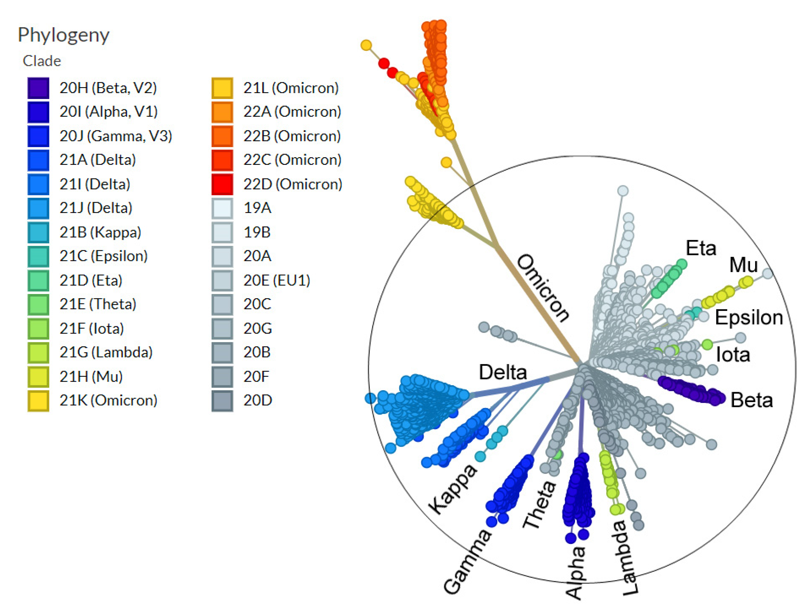
Figure 1. SARS-CoV-2 variants of concern shown on an unrooted phylogenetic tree, the branches of which are scaled by genetic divergence. This image was derived from Nextstrain (https://nextstrain.org/; 15 October 2022) under a CC-BY-4.0 license. The authors of this publication added annotations of the clades to the tree, as well as the centred black circle through the most distant non-Omicron variant.
Covid 03 00002 g001
Figure 2. Dynamics of the Omicron wave in Hong Kong; (a) velocity (daily case data) against the time (in days; day 1 = 1 January 2020), vmax = peak velocity of filtered data, v ¯ = average velocity of the effective phase; (b) acceleration against time, amax = maximum acceleration, amin = minimum acceleration (maximum deceleration), Δa = acceleration differential during the effective phase, TE = duration of the effective phase; (c) jerk against time, j ¯ = average jerk across the effective phase; (d) effectiveness against time, tE1 & tE2 = start and end of the effective phase, E ¯ = average effectiveness across the effective phase.
Covid 03 00002 g002
Figure 3. Running Line Method; (a) Box and Whisker plot of the logarithm of the land area (log A of countries shown in Appendix A); (b) log A against the percentile of land area; boundary values of log A, associated with the 30th and 70th percentile (central 40% percentile); (c) p-values associated with each line of separation, dividing the land area into large and small countries, against the %ile of land area; (d) enlarged section of c (central 40% percentile); (e) the medians of log ρ of small and large area countries at any separation line, including the difference of the medians, against the %ile of land area; (f) enlarged section of (e) (central 40% percentile).
Covid 03 00002 g003
Figure 4. Wave histogram (density diagram): number of waves per month against the time (in days; day 1 = 1 January 2020); bin width = number of days of the mean year divided by 12.
Covid 03 00002 g004
Figure 5. Correlations; (a) effectiveness E data of 1000 waves against the duration of the effective phase TE with associated isolines of ρ (=E/TE) and log ς (wave shape factor); (b) ρ against log ς; (c) effectiveness E against the duration of the effective phase TE separately for Omicron and pre-Omicron waves; (d) ρ against log ς separately for Omicron and pre-Omicron waves.
Covid 03 00002 g005
Figure 6. Regressions; (a) effectiveness E data of 1000 waves against time; (b) duration of the effective phase TE against time; (c) ρ against time; (d) log ς against time; (e) peak velocity vmax against time; (f) peak velocity per population (vmax/P) against time; note that the two bands with greater wave density, at approximately 750 and 925 days are Omicron waves.
Covid 03 00002 g006
Figure 7. Regressions; (a) effectiveness E data of 615 pre-Omicron (blue) and 385 Omicron (red) waves against time; (b) duration of the effective phase TE against time; (c) ρ against time; (d) log ς against time; (e) peak velocity vmax against time; (f) peak velocity per population (vmax/P) against time; “no trend” refers to p > 0.05.
Covid 03 00002 g007
Figure 8. Box and Whisker plots of effectiveness parameters such as duration of the effective phase TE, effectiveness E, ρ and log ς of 1000 COVID-19 waves, thereof 615 pre-Omicron and 385 Omicron waves.
Covid 03 00002 g008
Table 1. Statistical details of Figure 6 and Figure 7; R2 = coefficient of determination, r = effect size (Cohen’s f); p = probability value; TE = duration of the effective phase; E = effectiveness (of wave management); ρ = E/TE; log ς = wave shape factor; vmax = peak velocity; vmax/P = peak velocity per population P.
All WavesR2rEffectp-ValueStandard Error
log TE0.03580.1927smallp < 0.00010.3124
log E0.03510.1907smallp < 0.00010.4446
log ρ0.03710.1964smallp < 0.00010.7382
log ς0.01410.1195smallp = 0.00010.1489
log (vmax/P)0.12130.3715mediump < 0.00010.8719
log vmax0.03200.1818smallp < 0.00010.9794
pre-Omicron wavesR2reffectp-valuestandard error
log TE0.00010.0104very smallp > 0.050.3329
log E0.00440.0664very smallp > 0.050.4573
log ρ0.00190.0439very smallp > 0.050.7708
log ς0.00530.0727very smallp = 0.0360.1613
log (vmax/P)0.13050.3873mediump < 0.00010.7614
log vmax0.02620.1642smallp = 0.00010.9051
Omicron wavesR2reffectp-valuestandard error
log TE0.00070.0267very smallp > 0.050.2669
log E00.0058very smallp > 0.050.3985
log ρ0.00020.0146very smallp > 0.050.6478
log ς0.00220.0472very smallp > 0.0550.1269
log (vmax/P)0.05170.2334smallp < 0.00010.9336
log vmax0.06220.2575mediump < 0.00011.0193
Table 2. Comparison of medians of pre-Omicron (n = 615) and Omicron (n = 385) waves (wave ratio 8:5); U = U-statistic value of the Mann–Whitney test; p = probability value; r = effect size; TE = duration of the effective phase; E = effectiveness (of wave management); ρ = E/TE and log ς = wave shape factor; vmax = peak velocity; vmax/P = peak velocity per population P.
ParametersMedian Pre-OmicronMedian OmicronUprEffectInterpretation: Omicron Waves Have a … Median
log TE1.3801.25585,359<0.00010.279mediumsmaller
log E−2.334−2.12079,591<0.00010.328mediumgreater
log ρ−3.722−3.36881,110<0.00010.315mediumgreater
log ς0.0250.043107,0370.01080.096very smallgreater
log vmax2.9633.28396,037<0.00010.189smallgreater
log (vmax/P)−3.845−3.22973,844<0.00010.376largegreater
Table 3. Relationship between epidemiological parameters and geographical and socioeconomic data across all 1000 waves; P = population; A = land area; G = GDP per capita (GDP/P); I = educational index; D = population density (P/A); TE = duration of the effective phase; E = effectiveness; ρ = E/TE and logς = wave shape factor; vmax = peak velocity; vmax/P = peak velocity per population P; cut-off = value of P, A, G, I, or D that divides, e.g., P into two subsamples of low and high P with associated, e.g., E-values that are significantly different at the lowest possible p-value (cf. Figure 3c,d); n1,2 = sample sizes for the Mann–Whitney U test; U = U-statistic value of the Mann–Whitney test; p = probability value; r = effect size.
PCut-Offn1, Low Pn2, High PMedian, Low PMedian, High PUprEffectInterpretation
log TE6.5393376661.231.35288,571<0.00010.211smallmore P, longer duration
log E6.539337666−2.061−2.30581,296<0.00010.276mediummore P, less effective
log ρ6.539337666−3.254−3.66883,755<0.00010.254mediummore P, less effective
log ς6.9665194830.0420.022112,5110.00510.102smallmore P, less triangular
log (vmax/P)7.067594409−3.319−4.20452,960<0.00010.564largemore P, less relative cases
Acut-offn1, small An2, large Amedian, small Amedian, large AUpreffectinterpretation
log TE4.5843396631.2041.36286,818.5<0.00010.227smallmore A, longer duration
log E4.627352651−2.063−2.31982,163<0.00010.283mediummore A, less effective
log ρ4.627352652−3.246−3.68584,149<0.00010.267mediummore A, less effective
log ς4.9164295750.0450.025111,384.50.00850.097very smallmore A, less triangular
log (vmax/P)4.96460542−3.242−3.97669,799.5<0.00010.44largemore A, less relative cases
Gcut-offn1, low Gn2, high Gmedian, low Gmedian, high GUpreffectinterpretation
log TE−1.9663366631.2791.32299,2920.0050.109smallmore G, longer duration
log E−1.9476633360.0070.00588,280<0.00010.207smallmore G, less effective
log ρ−1.844416583−3.418−3.667101,392<0.00010.164smallmore G, less effective
log ς−1.7575114890.0230.039115,093.50.03080.079very smallmore G, more triangular
log (vmax/P)−1.947336665−4.568−3.31235,558<0.00010.682largemore G, more relative cases
Icut-offn1, low In2, high Imedian, low Imedian, high IUpreffectinterpretation
log TE0.6383385861.2551.36279,376.5<0.00010.198smallmore I, longer duration
log E0.638338586−2.058−2.33468,536.5<0.00010.308mediummore I, less effective
log ρ0.638338671−3.312−3.64387,807.5<0.00010.226smallmore I, less effective
log ς0.8056582620.0250.04673,681.50.00060.145smallmore I, more triangular
log (vmax/P)0.64335671−4.54−3.31536,844.5<0.00010.672largemore I, more relative cases
Dcut-offn1, low Dn2, high Dmedian, low Dmedian, high DUpreffectinterpretation
log TEin-significant
log E1.912487513−2.177−2.23135,079.50.02570.081very smallmore D, less effective
log ρ1.903484515−3.471−3.56115,6670.04880.072very smallmore D, less effective
log ςin-significant
log (vmax/P)1.974539463−3.814−3.409100,923.5<0.00010.191smallmore D, more relative cases
Table 4. Relationship between epidemiological parameters and geographical and socioeconomic data across all pre-Omicron waves; P = population; A = land area; G = GDP per capita (GDP/P); I = educational index; D = population density (P/A); TE = duration of the effective phase; E = effectiveness; ρ = E/TE and logς = wave shape factor; vmax = peak velocity; vmax/P = peak velocity per population P; cut-off = value of P, A, G, I, or D that divides, e.g., P into two subsamples of low and high P with associated, e.g., E-values that are significantly different at the lowest possible p-value (cf. Figure 3c,d); n1,2 = sample sizes for the Mann–Whitney U test; U = U-statistic value of the Mann–Whitney test; p = probability value; r = effect size.
PCut-Offn1, Low Pn2, High PMedian, Low PMedian, High PUprEffectInterpretation
log TE6.963023141.3011.44736,495.5<0.00010.23smallmore P, longer duration
log E6.63207409−2.15−2.43229,834<0.00010.295mediummore P, less effective
log ρ6.96302314−3.518−3.88534,911<0.00010.264mediummore P, less effective
log ςin-significant
log (vmax/P)7.067357260−3.566−4.33824,561<0.00010.471largemore P, less relative cases
Acut-offn1, small An2, large Amedian, small Amedian, large AUpreffectinterpretation
log TE4.6822104061.2551.44730,755.5<0.00010.279mediummore A, longer duration
log E4.628206410−2.123−2.4527,597<0.00010.347mediummore A, less effective
log ρ4.682210406−3.359−3.88328,867<0.00010.323mediummore A, less effective
log ςin-significant
log (vmax/P)4.959276341−3.404−4.12225,696<0.00010.454largemore A, less relative cases
Gcut-offn1, low Gn2, high Gmedian, low Gmedian, high GUpreffectinterpretation
log TEin-significant
log E−1.99207409−2.286−2.435,8050.00170.154smallmore G, less effective
log ρ−1.916227389−3.676−3.80238,7880.01170.121smallmore G, less effective
log ςin-significant
log (vmax/P)1.99208409−4.649−3.51414,107<0.00010.668largemore G, more relative cases
Icut-offn1, low In2, high Imedian, low Imedian, high IUpreffectinterpretation
log TE0.6182053681.3421.43131,0440.00040.177smallmore I, longer duration
log E0.618205413−2.241−2.41232,901.5<0.00010.223smallmore I, less effective
log ρ0.604199373−3.58−3.8728,214.5<0.00010.24smallmore I, less effective
log ςin-significant
log (vmax/P)0.632207407−4.639−3.50314,265.5<0.00010.661largemore I, more relative cases
Dcut-offn1, low Dn2, high Dmedian, low Dmedian, high DUpreffectinterpretation
log TE2.1054102061.4311.30136,7430.00850.13smallmore D, SHORTER duration
log E2.105410206−2.424−2.21636,434.50.00540.137smallmore D, MORE effective
log ρ2.073404213−3.818−3.55937,7060.01140.124smallmore D, MORE effective
log ςin-significant
log (vmax/P)1.833250367−3.99−3.68736,395<0.00010.207smallmore D, more relative cases
Table 5. Relationship between epidemiological parameters and geographical and socioeconomic data across all Omicron waves; P = population; A = land area; G = GDP per capita (GDP/P); I = educational index; D = population density (P/A); TE = duration of the effective phase; E = effectiveness; ρ = E/TE and logς = wave shape factor; vmax = peak velocity; vmax/P = peak velocity per population P; cut-off = value of P, A, G, I, or D that divides, e.g., P into two subsamples of low and high P with associated, e.g., E-values that are significantly different at the lowest possible p-value (cf. Figure 3c,d); n1,2 = sample sizes for the Mann–Whitney U test; U = U-statistic value of the Mann–Whitney test; p = probability value; r = effect size.
PCut-Offn1, Low Pn2, High PMedian, low PMedian, High PUprEffectInterpretation
log TE7.2262581271.1761.30112,861.50.00060.215smallmore P, longer duration
log E7.226258127−2.028−2.16813,078.50.00130.202smallmore P, less effective
log ρ7.226258127−3.2−3.47712,871.50.00060.214smallmore P, less effective
log ς7.2262581270.0510.03114,016.50.02140.144smallmore P, less triangular
log (vmax/P)6.349125261−2.792−3.4938522<0.00010.478largemore P, less relative cases
Acut-offn1, small An2, large Amedian, small Amedian, large AUpreffectinterpretation
log TEin-significant
log E4.482135250−1.988−2.11514,278.50.01280.154smallmore A, less effective
log ρ4.482135250−3.168−3.3914,425.50.01880.145smallmore A, less effective
log ςin-significant
log (vmax/P)4.952182203−2.868−3.58310,426.5<0.00010.436largemore A, less relative cases
Gcut-offn1, low Gn2, high Gmedian, low Gmedian, high GUpreffectinterpretation
log TE−1.662121741.191.27913,957.5<0.00010.243mediummore G, longer duration
log E−1.66212174−1.968−2.2311,065<0.00010.4largemore G, less effective
log ρ−1.707209177−3.173−3.5412,165<0.00010.342mediummore G, less effective
log ς−1.42671190.0310.06413,0040.00440.181smallmore G, more triangular
log (vmax/P)−1.648218168−3.74−2.7425889<0.00010.678largemore G, more relative cases
Icut-offn1, low In2, high Imedian, low Imedian, high IUpreffectinterpretation
log TE0.6591302181.0971.2799323.5<0.00010.342mediummore I, longer duration
log E0.659130218−1.838−2.1777005<0.00010.506largemore I, less effective
log ρ0.659130218−2.943−3.4827819<0.00010.448largemore I, less effective
log ς0.7312031450.0250.06711,5840.00070.213smallmore I, more triangular
log (vmax/P)0.765223163−3.688−2.6725432.5<0.00010.701largemore I, more relative cases
Dcut-offn1, low Dn2, high Dmedian, low Dmedian, high DUpreffectinterpretation
log TE1.9031871991.2041.25515,896.50.01350.146smallmore D, longer duration
log E1.903187198−2.017−2.12315,072.50.00160.186smallmore D, less effective
log ρ1.903187198−3.251−3.37815,401.50.00440.168smallmore D, less effective
log ςin-significant
log (vmax/P)1.974207179−3.4−3.01914,8780.00080.197smallmore D, more relative cases
Disclaimer/Publisher’s Note: The statements, opinions and data contained in all publications are solely those of the individual author(s) and contributor(s) and not of MDPI and/or the editor(s). MDPI and/or the editor(s) disclaim responsibility for any injury to people or property resulting from any ideas, methods, instructions or products referred to in the content.