Machine Learning Prediction of Henry’s Law Constant for CO₂ in Ionic Liquids and Deep Eutectic Solvents

Abstract

Ionic liquids (ILs) and deep eutectic solvents (DESs) have been extensively studied as absorbents for CO₂ capture, demonstrating high efficiency in this role. To optimize the search for compounds with superior absorption properties, theoretical approaches, including machine learning methods, are highly relevant. In this study, machine learning models were developed and applied to predict Henry’s law constants for CO₂ in ILs and DESs, aiming to identify systems with the best absorption performance. The accuracy of the models was assessed in interpolation tasks within the training set and extrapolation beyond its domain. The optimal predictive models were built using the CatBoost algorithm, leveraging CDK molecular descriptors for ILs and RDKit descriptors for DESs. To define the applicability domain of the models, the SHAP-based leverage method was employed, providing a quantitative characterization of the descriptor space where predictions remain reliable. The developed models have been integrated into the web platform chem-predictor, where they can be utilized for predicting absorption properties.

1. Introduction

Carbon capture, utilization, and storage (CCUS) technologies play a key role in mitigating global climate change caused by greenhouse gas emissions [1,2]. These technologies aim to reduce atmospheric CO₂ concentrations by capturing it from industrial sources, such as flue gases from power plants and manufacturing facilities. Once captured, CO₂ can either be converted into valuable products [3] or securely sequestered to prevent its release back into the atmosphere [4].

Although CO₂ capture using aqueous monoethanolamine solutions has been widely applied in industry for decades, its high energy demand and significant solvent losses during regeneration have driven the search for alternative absorbents [5,6,7]. Developing efficient CO₂ capture and separation methods remains an urgent challenge for the scientific community and is a key topic in chemical engineering [8].

Ionic liquids (ILs), composed of organic cations and organic or inorganic anions, represent a unique class of compounds that have attracted considerable attention due to their exceptional properties. They remain liquid over a wide temperature range, including ambient conditions, and exhibit negligible vapor pressure, making them non-volatile. Additionally, ILs are thermally stable, non-flammable, and chemically versatile, allowing for a broad spectrum of ion combinations [9]. These properties make them promising candidates for reducing the environmental risks associated with various technological processes, including acid gas capture [10,11,12,13,14,15,16] and gas separation, which is crucial for natural gas purification [17,18]. Moreover, the non-volatility of ILs allows captured CO₂ to be easily released from the saturated solvents, resulting in lower energy consumption and reduced environmental impact compared to conventional amine scrubbing methods.

Deep eutectic solvents (DESs) have emerged as new-generation solvents that serve as potential alternatives to conventional solvents in various industrial applications. Their advantages include ease of synthesis, versatility, and superiority over both industrial solvents and ILs [19]. DESs are formed as mixtures of hydrogen bond acceptors (HBAs) and hydrogen bond donors (HBDs) [20], creating eutectic systems with melting points lower than those of the individual components. These mixtures exhibit negative deviations from thermodynamic ideality due to enthalpic interactions [21]. Compared to ILs, DESs offer the benefits of lower cost and simpler preparation, further enhancing their attractiveness as CO₂ absorbents.

CO₂ solubility is typically described by Henry’s law, where the key parameter is Henry’s constant (${\mathit{H}}_{\mathit{x}}$), expressed on a molar fraction scale. This constant depends solely on temperature and solvent nature, with higher ${\mathit{H}}_{\mathit{x}}$ values indicating lower solubility and vice versa. Theoretical approaches for predicting Henry’s constants are of significant interest, particularly in the context of absorption systems. In recent years, quantitative structure–property relationship (QSPR) models employing various methods have been developed to estimate CO₂ solubility in ILs and DESs.

For example, in a study by [22], a dataset of 297 experimental data points for 34 ILs was used, with $S\sigma$-profiles (surface area of electrostatic potential and charge distribution region) as descriptors. Models based on multiple linear regression (MLR), support vector machines (SVMs), and extreme learning machines (ELMs) demonstrated that ELMs achieved the best performance, with an average absolute relative deviation (AARD) of 4.24% on the test set. Another study [23] developed two QSPR models for predicting H_x in 32 ILs using MLR and SVM, achieving AARDs of 6.33% and 4.42%, respectively. Wu et al. [24] used 160 experimental data points for 32 imidazolium-based ILs in the temperature range of 283–350 K. Their multilayer perceptron (MLP) model, which incorporated 11 structural descriptors and temperature as a variable, achieved an RMSE of 0.7915 MPa. Zhang et al. [25] combined 132 experimental Henry’s constants with 84 values computed using molecular dynamics and trained models using RDKit descriptors, where the MLP model achieved the lowest MAE of 0.3023 MPa.

Additionally, a dataset of Henry’s constants for 20,000 ILs was generated using the Conductor-like Screening Model for Real Solvents (COSMO-RS) method [26]. This dataset was employed to construct a Gaussian process regression model with 12 filtered descriptors, yielding an RMSE of 1.5 MPa. However, as noted by Liu et al. [27], COSMO-RS-derived Henry’s constants can exhibit significant systematic deviations that require correction. The same study developed a COSMO-RS model tested on 132 experimental CO₂ Henry’s constants in DESs, yielding absolute relative deviations (ARDs) in the range of 13.7–36.3%.

Two major limitations are evident in the reviewed studies. First, studies relying on limited experimental datasets (containing fewer than 50 absorbents) inherently have a narrow applicability domain. Second, model performance evaluation in most of these studies is imprecise due to random dataset splitting, where the same absorbents appear in both training and test sets. This leads to overly optimistic results that do not reflect true model generalization. Only one study [24] employed the leave-one-compound-out protocol, where each IL (including all its data points at different temperatures) was sequentially used as the test set. This analysis revealed significantly higher errors compared to random splits, with the best model exhibiting an MAE of 1.6694 MPa.

To address these limitations, our study employed the largest possible dataset of CO₂ Henry’s constants for ILs and DESs, expanding it by incorporating structurally similar compounds to improve the models’ applicability domains. Furthermore, special attention was given to data-splitting strategies and cross-validation protocols during model evaluation to ensure a true assessment of generalization ability. Through this approach, we successfully developed publicly accessible models for predicting CO₂ Henry’s constants in ILs and DESs.

2. Materials and Methods

2.1. Datasets

The slope of the CO₂ solubility curve in the absorbent corresponds to the Henry’s law constant based on the mole fraction (${\mathit{H}}_{\mathit{x}}$), as defined by the following relationship (1):

$$H_x(p,T)=\underset{x_{C{O}_2}\to 0}{lim}{\displaystyle \frac{f_{C{O}_2}^{\mathrm{liq}}}{x_{C{O}_2}}}\cong {\displaystyle \frac{p{\varphi }_{C{O}_2}}{x_{C{O}_2}}},$$

(1)

where $f_{C{O}_2}^{\mathrm{liq}}$, $x_{C{O}_2}$, and ${\varphi }_{C{O}_2}$ are the fugacity, mole fraction, and fugacity coefficient of CO₂ in the liquid phase, respectively; p is the pressure and T is the temperature.

The dataset of Henry’s law constants for CO₂ in absorbents was compiled from the literature and is provided in the Supplementary Information, along with references to the original sources. The dataset for ILs as absorbents consists of 311 data points for 59 ILs, with values ranging from 0.75 to 35 MPa, measured at temperatures between 283 and 500 K (referred to as the “ILs dataset”).

The dataset of ${\mathit{H}}_{\mathit{x}}$ in DESs comprises 346 data points for 72 DESs, with Henry’s law constant values ranging from 2.95 to 77 MPa. The molar fraction of HBDs in the mixtures varies between 0.3 and 0.94, while the temperature range extends from 293 to 363 K (referred to as the “DESs dataset”).

To the best of our knowledge, this is the largest publicly available database of ILs and DESs to date. The SMILES representations for ILs, as well as for HBAs and HBDs, were generated based on their chemical names using the OPSIN online service [28].

A straightforward procedure was employed to identify and eliminate duplicates within the collected datasets [29]. Initially, the entire dataset was used to develop a regression model. Subsequently, structures with multiple property values were filtered out, and data points exhibiting the largest deviations from the model were removed.

2.2. Molecular Descriptors

In this study, well-established and widely used descriptor sets were selected to automate the descriptor generation process and ensure the seamless integration of the model into an autonomous mode on a web platform. Three open-source cheminformatics tools were utilized: Mold2 [30], CDK (Chemistry Development Kit) [31], and RDKit [32]. The Mold2 package comprises 777 molecular descriptors. The CDK software (version 2.8) generates a collection of 222 two-dimensional descriptors. RDKit provides more than 200 descriptors. These tools offer a diverse range of descriptors capturing the chemical and topological properties of molecules, which can be broadly classified into the following categories: atomic characteristics, structural properties, physicochemical parameters, basic electronic information, and molecular complexity.

The inclusion of an excessive number of irrelevant features can introduce noise and distract the model, particularly in low-data scenarios [33]. Therefore, after descriptor generation, a filtering step was applied to remove those that were ineffective in describing the structure–property relationships. Descriptors with constant values and absolute values exceeding 999,999 were eliminated. Additionally, descriptors with a high pairwise correlation coefficient (above 0.95) were grouped, and only the first descriptor from each group was retained for model development. The final number of selected features varied depending on the descriptor set.

For ILs, descriptors were calculated for the ion pair, while for mixtures, the descriptors of each component were averaged according to their molar fraction.

2.3. Machine Learning Algorithms

Prior to selecting algorithms for modeling, we carried out an initial comparison between representation learning approaches (Directed Message-Passing Neural Networks (D-MPNNs) [34] and Transformer Convolutional Neural Fingerprint (TransCNF) [35]) and traditional machine learning algorithms such as Random Forest [36] and CatBoost [37] (see Figure S1). Traditional methods showed comparable performance with TransCNF, but we favored them because they are among the most widely used solutions due to their versatility and interpretability.

Random Forest employs ensemble learning (combining multiple decision trees), which reduces the risk of overfitting and enhances the model’s robustness to noise in the data.

CatBoost effectively addresses the overfitting issues inherent in traditional gradient boosting by utilizing a unique approach to categorical feature processing and estimating leaf values through random permutations during tree construction. CatBoost has already been successfully applied to mixtures [38] and chemical reactions [39], demonstrating its effectiveness when trained on limited data.

These algorithms generally outperform neural network approaches on small datasets, making them particularly suitable for our task. Moreover, they require minimal data preprocessing and exhibit high training efficiency.

In this study, model hyperparameters were optimized using Optuna [40].

2.4. Model Validation

An essential aspect of understanding the predictive capability of a model is the division of experimental data into a training dataset, used for model calibration, and a validation dataset, used to assess the model’s performance and estimate prediction uncertainty. All models developed in this study underwent a 5-fold cross-validation (5-CV) procedure. In 5-CV, the dataset was split into five approximately equal subsets, and the model was trained and validated five times. During each training iteration, one subset was used as the validation set, while the remaining four subsets were combined into a training set. Cross-validation provides predictions for all data points, distinguishing it from the more conventional approach of making a single prediction based on a random train–test split.

For ionic liquids and mixtures, cross-validation can be performed using three different strategies [41,42]: “Data-points” validation, “Mixture” validation, and “Components” validation. Since the “Components” validation protocol requires a large dataset with a diverse set of molecules, in this study, models were validated using only the first two protocols.

The “Data-points” validation protocol (hereafter referred to as random splitting) evaluates the model within the training set, interpolating predictions for new mixture concentrations or temperatures. The “Mixture” validation protocol (hereafter referred to as strict splitting) assesses the model’s ability to extrapolate, predicting the properties of new mixtures or ionic liquids composed of components (ions) already present in the training set. Three statistical metrics were used to evaluate model performance: the root mean square error (RMSE), the coefficient of determination ($R^2$), and the average absolute relative deviation (AARD):

$$\mathrm{RMSE}=\sqrt{{\displaystyle \frac{1}{n}}\sum _{i=1}^n{(H_{x_i}^{\exp }-H_{x_i}^{\mathrm{pred}})}^2}$$

(2)

$$R^2=1-{\displaystyle \frac{{\sum }_{i=1}^n{(H_{x_i}^{\exp }-H_{x_i}^{\mathrm{pred}})}^2}{{\sum }_{i=1}^n{(H_{x_i}^{\exp }-{\overline{H_x}}^{\exp })}^2}}$$

(3)

$$\mathrm{AARD}={\displaystyle \frac{100\%}{n}}\sum _{i=1}^n{\displaystyle \frac{|H_{x_i}^{\exp }-H_{x_i}^{\mathrm{pred}}|}{H_{x_i}^{\exp }}}$$

(4)

where n is the number of data points, $H_{x_i}^{\exp }$ is the experimental Henry’s constant value, and $H_{x_i}^{\mathrm{pred}}$ is the predicted Henry’s constant value.

2.5. SHAP-Based Leverage

The leverage method, widely used for outlier diagnostics, has proven to be an effective tool due to its analytical rigor and clear visualization using Williams plots [43]. This method involves calculating standardized residuals, which reflect the deviation of model predictions from experimental data, as well as leverage values, defined as the diagonal elements of the influence matrix (hat matrix). The influence matrix, based on linear algebra principles, quantitatively assesses the degree of influence each data point has on the model. However, the classical leverage method has a significant limitation: it assumes a linear relationship between descriptors and the target variable, making it less applicable to nonlinear models, where such assumptions may lead to overly optimistic estimates.

A SHAP-based leverage approach, using SHapley Additive exPlanations (SHAP) values, was previously proposed [44] to evaluate the contribution of each feature to the model’s prediction. Leverage values (L) in this approach are computed as the sum of the absolute SHAP values for each data point:

$$L_i=\sum _{j=1}^d\left|{\mathrm{SHAP}}_{ij}\right|$$

(5)

where ${\mathrm{SHAP}}_{ij}$ represents the contribution of the j-th descriptor to the i-th data point, and d is the number of descriptors.

3. Results and Discussion

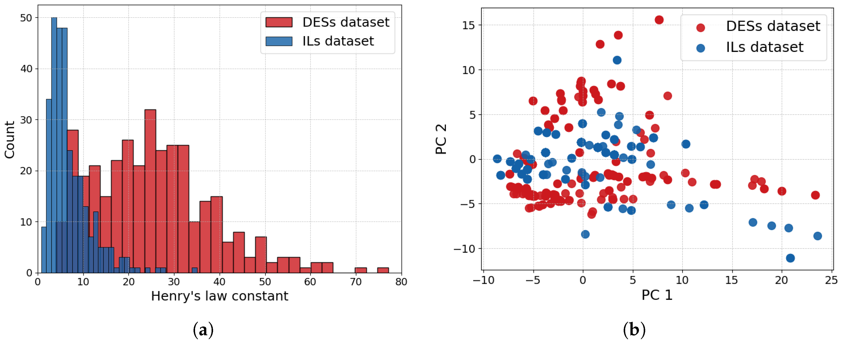
3.1. Dataset Analysis

The structural diversity of compounds plays a key role in improving the predictive power and generalizability of models. However, excessive diversity can negatively impact prediction accuracy. In this study, we analyzed the IL and DES datasets to assess their chemical space distribution and the distribution of Henry’s constant values.

The distributions of Henry’s constant values for the ILs and DESs datasets (Figure 1a) exhibit different patterns. The IL distribution is concentrated at low values (0–15 MPa), with a sharp decline in frequency as the constant increases. In contrast, the DES distribution is broader and right-skewed, with a greater number of values in the 10–50 MPa range and occasional outliers above 60 MPa. The ILs dataset exhibits a more pronounced left skew, whereas the DESs distribution is closer to normal but with a slight right skew. A comparison of these distributions indicates that, on average, CO₂ is more soluble in ILs than in DESs. This can be attributed to the stronger electrostatic and dispersion interactions between ILs and CO₂ compared to DESs. Additionally, ILs often contain large anions, such as bis(trifluoromethanesulfonyl)imide and hexafluorophosphate, which are highly polarizable and enhance CO₂ interactions.

Principal Component Analysis (PCA) was employed to explore dataset structure. PCA is a linear projection method that identifies fundamental variables (principal components), which are eigenvectors of the covariance matrix of the multivariate space. The first two PCA dimensions capture most of the variation in the original dataset. RDKit descriptors were used as compressed features for both datasets.

PCA analysis revealed that the structures of DESs and ILs exhibit overlapping yet distinct distributions (Figure 1b). While no clear separation into two distinct clusters was observed, a significant shift in the center (around zero) was noted: DES structures were more frequently found in the negative region of PC2, whereas ILs were predominantly found in the positive region.

Since PCA reflects real differences in descriptor distributions, this divergence may introduce challenges in the generalization of machine learning models. To assess the feasibility of merging these datasets into a unified model, it is necessary to evaluate prediction quality separately for each subset.

Additionally, Tanimoto similarity was calculated for the absorbent structures in both datasets, and Empirical Cumulative Distribution Functions (ECDFs) were constructed for the mean similarity values (Figure S2). For this, Extended Connectivity Fingerprints (ECFPs) (radius 2, 2048-bit) were computed using RDKit, and the mean Tanimoto similarity between each molecule and all others in the corresponding dataset was determined.

The analysis revealed that ILs exhibit a broader similarity distribution, with most molecules showing Tanimoto similarity values in the 0.2–0.6 range. In contrast, the DES distribution was more compact, with similarity values predominantly in the 0.1–0.3 range. This indicates lower intragroup similarity and higher structural diversity in the DES dataset compared to the relatively homogeneous ILs dataset.

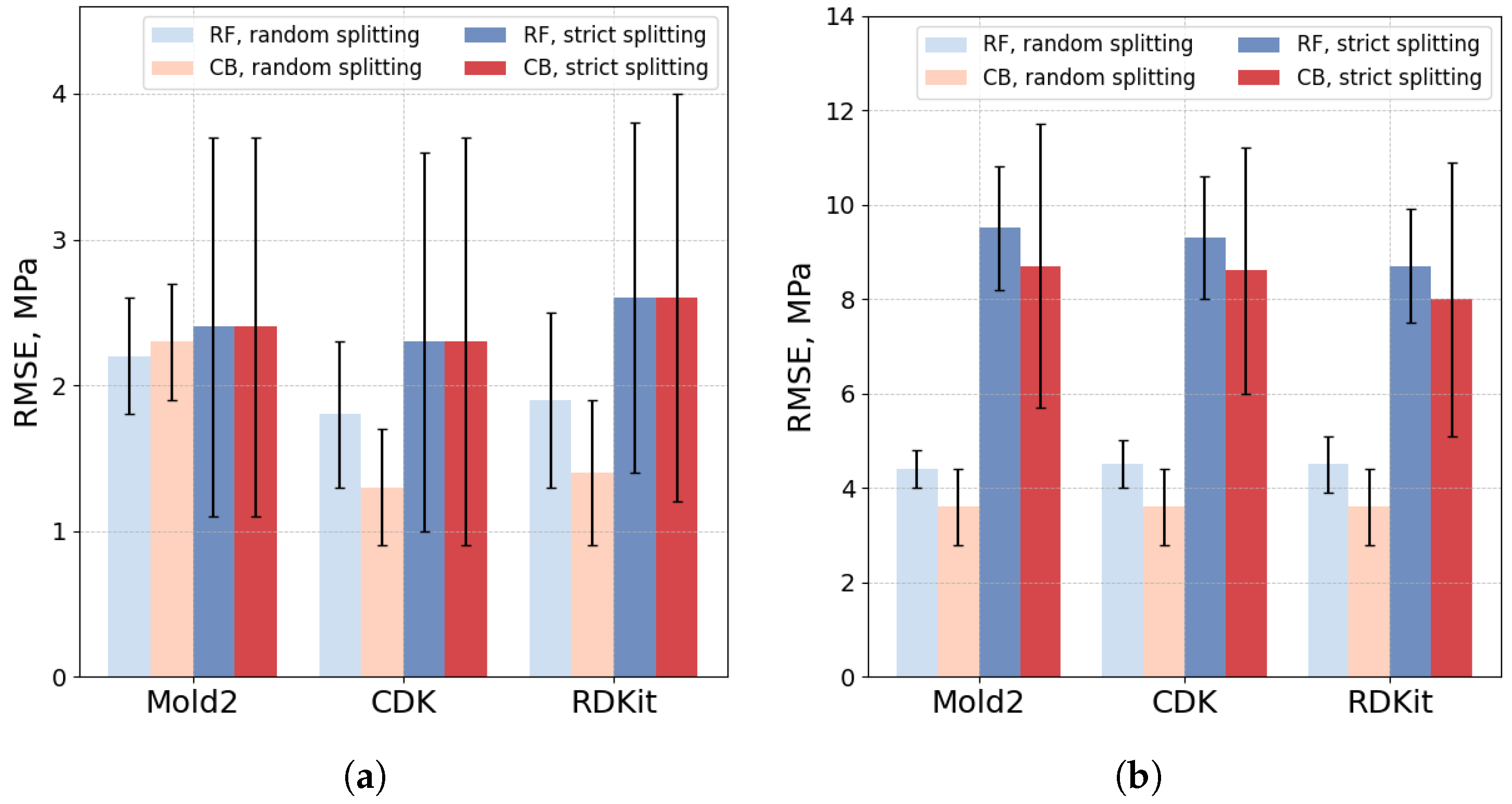
3.2. Models for Individual Datasets

The next stage of this study involved identifying the most suitable algorithm and descriptor set for predicting the Henry’s constant of CO₂ in ILs and DESs. The statistical parameters of models developed using different methods and evaluated via two types of 5-fold cross-validation are presented in Table S1, while their RMSE values are shown in Figure 2.

Figure 2 illustrates that strict data splitting during validation leads to higher RMSE values compared to random splitting. In random splitting, the same ionic liquid (or DES) at different temperatures (or concentrations) may appear in different folds during cross-validation. This allows the model to “recognize” certain compounds in the test sets, leading to more accurate property predictions.

Strict splitting, in contrast, creates more challenging conditions for the model by partitioning data based on chemical diversity, which better reflects real-world application scenarios. Consequently, model performance exhibits greater variability, as indicated by increased standard deviation. This can be attributed to the varying complexity of test sets, which depends on the degree of similarity between the test compounds and those in the training set.

It is also important to note that errors differ depending on the type of absorbent. For the IL dataset, the average RMSE is 2.3 MPa, whereas for DESs, it increases to 8 MPa. This is due not only to the broader range of Henry’s constant values in DES mixtures compared to ILs but also to the fact that DESs consist of two components with variable concentrations, adding additional complexity to their modeling. This is further supported by the more significant increase in error when transitioning from random to strict data splitting for DESs compared to ILs.

The CatBoost algorithm outperforms Random Forest in most cases, yielding lower RMSE values and indicating its higher accuracy for the given tasks. Additionally, RDKit and CDK descriptors demonstrate lower RMSE values compared to Mold2. Moving forward, only strict data splitting was considered for selecting the final models. The optimal combination for the IL dataset was CatBoost with CDK descriptors, whereas for the DES dataset, the best performance was achieved using CatBoost with RDKit descriptors.

3.3. Models for Combined Datasets

Next, we investigated the potential advantages of increasing the chemical diversity of the training set by merging IL and DES data. Previous studies have shown that this approach yielded positive results when modeling the mole fraction solubility of CO₂ in DESs [45], where the training set was augmented with pure IL data. However, a similar strategy did not lead to significant improvements in predicting the viscosity of DESs [38].

To ensure a reliable comparison, we employed 5-CV with strict data splitting for each subset. The test folds remained fixed, while the training sets were always supplemented with all data from the other subset (i.e., all DES data were added to the IL training set and vice versa). For reproducibility, the random seed value for data partitioning was kept constant. This allowed us to accurately compare model performance on the same test sets used for individual datasets (as described in Section 3.2).

For the IL dataset, this strategy increased the RMSE from 2.3 to 2.7 MPa after expanding the training set. For DESs, the RMSE increased from 8.0 to 8.4 MPa. Thus, the blind merging of datasets does not improve model generalization. Consequently, developing a global model by combining ILs and DESs into a single dataset is not advisable, as individual models exhibit superior performance.

Next, the Tanimoto similarity index was used to selectively add only structurally similar components to each dataset. For this, the average Tanimoto similarity was calculated for each DES structure with all IL structures, and vice versa (Figure S3).

Ideally, merging should occur when Tanimoto similarity values exceed 0.3. However, at this threshold, no DES structures were recommended for inclusion in the IL set, nor vice versa. Lowering the threshold to 0.10 allowed the addition of 67 data points corresponding to 27 unique DESs to the IL dataset. The retrained CatBoost:CDK model slightly improved RMSE to 2.2 MPa. For DESs, 45 data points from nine ILs were added, and the retrained CatBoost:RDKit model reduced the average RMSE to 7.9 MPa. This indicates that selectively incorporating structurally similar compounds expanded the chemical diversity of the dataset while slightly enhancing model performance.

After adding the selected ILs and DESs to their respective datasets, we retrained the best models to finalize their performance metrics under the two validation protocols. Scatter plots and statistical indicators illustrating the effectiveness of the best models in predicting the Henry’s constant of CO₂ in ILs and DESs under different validation protocols are presented in Figure 3. Notably, when evaluating the extrapolation capabilities of the models for both datasets, there was a consistent trend of underestimating the predicted Henry’s constants for absorbents with low CO₂ solubility.

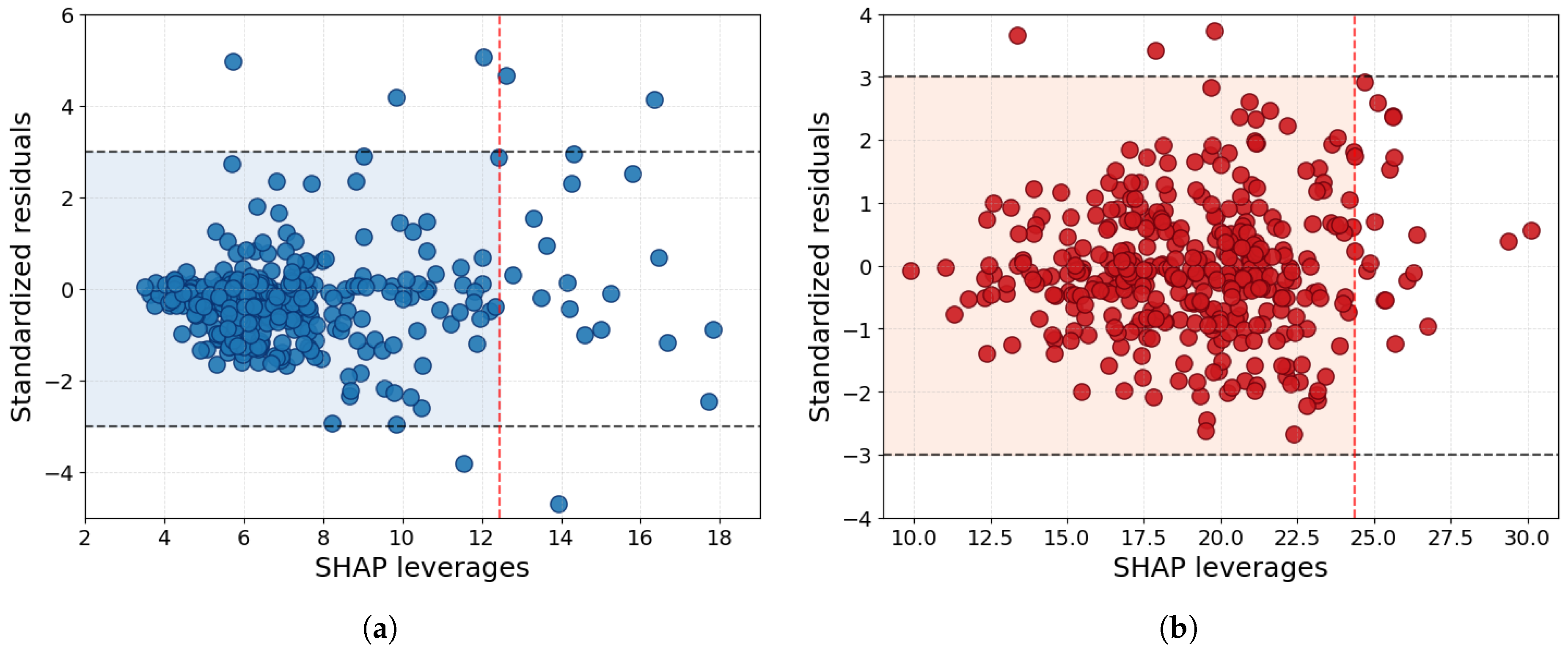
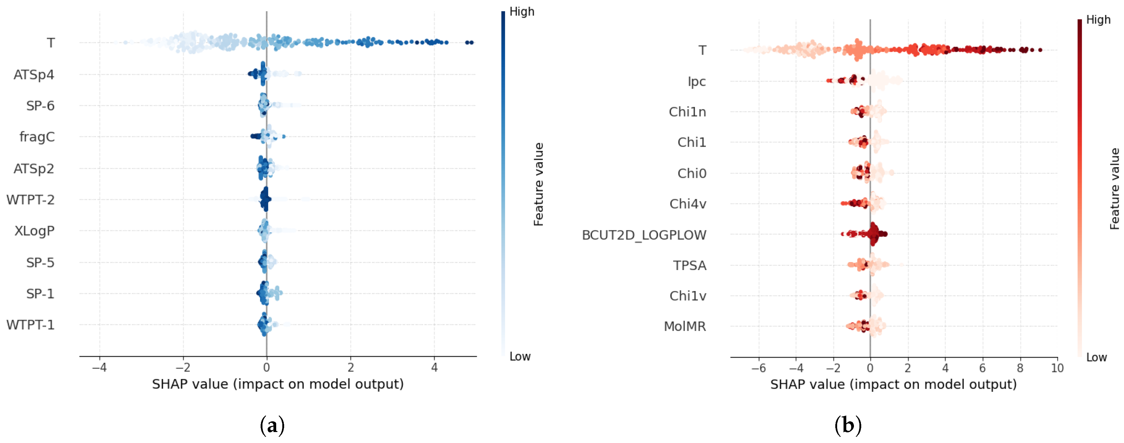
3.4. Applicability Domain and Feature Importance

To identify outliers in the datasets and establish the range of compounds suitable for reliable predictions, the applicability domain was assessed using SHAP leverage values for the best models. For a more robust evaluation, the analysis was conducted using 5-CV. To account for model variability during cross-validation, SHAP leverage values from each test set were aggregated, and the results were presented in a Williams plot (Figure 4).

Defining the reliable zone (shaded area) helps identify data points that align with the model’s expectations and fall within statistical reliability, facilitating accurate assessment and interpretation of the dataset. For the IL and DES datasets, the critical SHAP leverage values ($L^{*}$) were determined as 12.3 and 24.4, respectively. In the IL dataset, 19 data points corresponding to 8 compounds exceeded the threshold $L^{*}$, while in the DES dataset, 20 data points corresponding to 10 mixtures surpassed this limit. This suggests that predictions for these compounds may be less reliable.

In the IL dataset, the outliers included five salts based on the bis(trifluoromethanesul- fonyl)imide anion and three mixtures where butyltripropylammonium salts were used as HBAs. In the DES dataset, the identified outlier structures were more diverse, comprising mixtures based on choline chloride, betaine, biphenylmethane, L-proline, cetyltrimethylammonium bromide, and two ionic liquids with imidazolium cations.

In particular, the standardized residuals for these outliers were not excessively large. This suggests that compounds with high leverage values represent unusual but valid samples that the model interprets correctly, indicating a strong generalization capability.

The number of predicted CO₂ Henry’s constants falling outside the standardized residual range was minimal; however, most such cases were observed in the IL dataset. This could indicate potential experimental data errors for these compounds.

To evaluate the contribution of molecular descriptors to the prediction of the Henry’s law constant for CO₂, SHAP was used to interpret the trained models. Below, we present an analysis of the ten most important features identified for each model (Figure 5).

In both cases, temperature (T) was found to have the greatest impact on the model predictions, which supports the physicochemical plausibility of the models: as temperature increases, CO₂ solubility decreases, resulting in higher predicted values of the Henry’s constant.

For IL-based absorbents, the most influential descriptors included the autocorrelation indices ATSp4 and ATSp2, which capture interactions of atomic properties (e.g., polarizability) over specific bond distances. The WTPT-2 and WTPT-1 descriptors, associated with weighted topological paths, also played a significant role. Additionally, spectral indices such as SP-6, SP-5, and SP-1 highlighted the importance of the molecular graph’s spectral characteristics. The XLogP descriptor, which reflects molecular lipophilicity, contributed significantly to this outcome. Indeed, compounds with higher lipophilicity exhibited higher predicted Henry’s constants, consistent with the lower solubility of polar gases in nonpolar environments.

For DES systems, several RDKit topological descriptors were identified as key contributors. These included Ipc (information content index of connectivity) and a series of Chi indices (Chi0, Chi1, Chi1n, Chi1v, Chi4v), which reflect the molecular graph’s structure and branching. BCUT2D-LOGPLOW, a descriptor related to molecular polarity and charge distribution, and TPSA (topological polar surface area) further underscored the importance of polar interactions in CO₂ retention. The MolMR (molecular refractivity) descriptor reflected the influence of both volumetric and electronic properties of the molecules.

Thus, in both IL and DES systems, the models exhibited interpretable behavior by accounting for physicochemical (temperature, polarity, lipophilicity) and structural (topological, autocorrelation, spectral) molecular characteristics. This demonstrates that despite the different natures of ILs and DESs, the key patterns governing CO₂ solubility remain consistent and reproducible in predictive modeling.

4. Conclusions

In this study, individual models were developed for predicting the Henry’s constant of CO₂ in ILs and DESs. The feasibility of expanding training datasets by merging IL and DES datasets was explored. The most effective dataset expansion was observed when utilizing the average Tanimoto similarity index, which, at specific threshold values, improved the predictive performance of individual models. Compared to the Random Forest method, the proposed CatBoost-based models demonstrated higher accuracy. The best performance for ILs was achieved using CatBoost in combination with CDK descriptors, while for DESs, the best results were obtained with RDKit descriptors.

Model performance was assessed using both interpolation and extrapolation-based data splitting strategies, providing a practical evaluation of potential prediction errors for CO₂ Henry’s constant in next-generation absorbents. Despite differences in errors between the two types of absorbents (RMSE of 2.8 MPa for ILs and 7.7 MPa for DESs, as determined through rigorous model evaluation), these errors did not exceed 10% of the variability range of Henry’s constant values in the studied datasets.

As a result of this theoretical study, an online version of the developed models has been made available for use without registration at: http://chem-predictor.isc-ras.ru/ionic/ (accessed on 29 May 2025).

Besides high CO₂ solubility, the practical application of next-generation absorbents requires consideration of the thermodynamic characteristics of desorption. The energy intensity of sorbent regeneration can significantly limit their industrial implementation. In the future, models should take into account not only solubility parameters but also factors related to the reversibility of the process and the energy costs of CO₂ desorption, for example, by predicting the enthalpy of dissolution.

References

1. Lin, Q.; Zhang, X.; Wang, T.; Zheng, C.; Gao, X. Technical perspective of carbon capture, utilization, and storage. Engineering 2022, 14, 27–32. [Google Scholar] [CrossRef]
2. Gao, W.; Liang, S.; Wang, R.; Jiang, Q.; Zhang, Y.; Zheng, Q.; Xie, B.; Toe, C.Y.; Zhu, X.; Wang, J.; et al. Industrial carbon dioxide capture and utilization: State of the art and future challenges. Chem. Soc. Rev. 2020, 49, 8584–8686. [Google Scholar] [CrossRef]
3. LeClerc, H.O.; Erythropel, H.C.; Backhaus, A.; Lee, D.S.; Judd, D.R.; Paulsen, M.M.; Ishii, M.; Long, A.; Ratjen, L.; Gonsalves Bertho, G.; et al. The CO2 Tree: The Potential for Carbon Dioxide Utilization Pathways. ACS Sustain. Chem. Eng. 2024, 13, 5–29. [Google Scholar] [CrossRef]
4. Snæbjörnsdóttir, S.Ó.; Sigfússon, B.; Marieni, C.; Goldberg, D.; Gislason, S.R.; Oelkers, E.H. Carbon dioxide storage through mineral carbonation. Nat. Rev. Earth Environ. 2020, 1, 90–102. [Google Scholar] [CrossRef]
5. Chai, S.Y.W.; Ngu, L.H.; How, B.S. Review of carbon capture absorbents for CO2 utilization. Greenh. Gases Sci. Technol. 2022, 12, 394–427. [Google Scholar] [CrossRef]
6. Wu, H.; Zhang, X.; Wu, Q. Research progress of carbon capture technology based on alcohol amine solution. Sep. Purif. Technol. 2024, 333, 125715. [Google Scholar] [CrossRef]
7. Xu, Y.; Zhang, R.; Zhou, Y.; Hu, D.; Ge, C.; Fan, W.; Chen, B.; Chen, Y.; Zhang, W.; Liu, H.; et al. Tuning ionic liquid-based functional deep eutectic solvents and other functional mixtures for CO2 capture. Chem. Eng. J. 2023, 463, 142298. [Google Scholar] [CrossRef]
8. Zhao, K.; Jia, C.; Li, Z.; Du, X.; Wang, Y.; Li, J.; Yao, Z.; Yao, J. Recent advances and future perspectives in carbon capture, transportation, utilization, and storage (CCTUS) technologies: A comprehensive review. Fuel 2023, 351, 128913. [Google Scholar] [CrossRef]
9. Zhang, Z.y.; Wang, X.; He, Q.; Sun, Z. Chemical accuracy prediction of molecular solvation and partition in ionic liquids with educated estimators. J. Mol. Liq. 2023, 391, 123202. [Google Scholar] [CrossRef]
10. Blanchard, L.A.; Hancu, D.; Beckman, E.J.; Brennecke, J.F. Green processing using ionic liquids and CO2. Nature 1999, 399, 28–29. [Google Scholar] [CrossRef]
11. Aghaie, M.; Rezaei, N.; Zendehboudi, S. A systematic review on CO2 capture with ionic liquids: Current status and future prospects. Renew. Sustain. Energy Rev. 2018, 96, 502–525. [Google Scholar] [CrossRef]
12. Godény, M.; Schröder, C. Reactive Molecular Dynamics in Ionic Liquids: A Review of Simulation Techniques and Applications. Liquids 2025, 5, 8. [Google Scholar] [CrossRef]
13. Wang, C.; Luo, X.; Zhu, X.; Cui, G.; Jiang, D.E.; Deng, D.; Li, H.; Dai, S. The strategies for improving carbon dioxide chemisorption by functionalized ionic liquids. RSC Adv. 2013, 3, 15518–15527. [Google Scholar] [CrossRef]
14. Elmobarak, W.F.; Almomani, F.; Tawalbeh, M.; Al-Othman, A.; Martis, R.; Rasool, K. Current status of CO2 capture with ionic liquids: Development and progress. Fuel 2023, 344, 128102. [Google Scholar] [CrossRef]
15. Wen, S.; Zhang, X.; Wu, Y. Efficient Absorption of CO2 by Protic-Ionic-Liquid Based Deep Eutectic Solvents. Chem.-Asian J. 2024, 19, e202400234. [Google Scholar] [CrossRef]
16. Wu, Y.; Xu, J.; Mumford, K.; Stevens, G.W.; Fei, W.; Wang, Y. Recent advances in carbon dioxide capture and utilization with amines and ionic liquids. Green Chem. Eng. 2020, 1, 16–32. [Google Scholar] [CrossRef]
17. Huo, M.; Peng, X.; Zhao, J.; Ma, Q.; Cai, R.; Deng, C.; Liu, B.; Sun, C.; Chen, G. Mixed solvent of alcohol and protic ionic liquids for CO capture: Solvent screening and experimental studies. Int. J. Hydrogen Energy 2023, 48, 33173–33185. [Google Scholar] [CrossRef]
18. Ma, C.; Wang, N.; Xie, Y.; Ji, X. Hybrid solvents based on ionic liquids/deep eutectic solvents for CO2 separation. Sci. Talks 2023, 6, 100220. [Google Scholar] [CrossRef]
19. Prabhune, A.; Dey, R. Green and sustainable solvents of the future: Deep eutectic solvents. J. Mol. Liq. 2023, 379, 121676. [Google Scholar] [CrossRef]
20. Abbott, A.P.; Capper, G.; Davies, D.L.; Rasheed, R.K.; Tambyrajah, V. Novel solvent properties of choline chloride/urea mixtures. Chem. Commun. 2003, 70–71. [Google Scholar] [CrossRef]
21. Abranches, D.O.; Coutinho, J.A. Everything you wanted to know about deep eutectic solvents but were afraid to be told. Annu. Rev. Chem. Biomol. Eng. 2023, 14, 141–163. [Google Scholar] [CrossRef]
22. Kang, X.; Liu, C.; Zeng, S.; Zhao, Z.; Qian, J.; Zhao, Y. Prediction of Henry’s law constant of CO2 in ionic liquids based on SEP and Sσ-profile molecular descriptors. J. Mol. Liq. 2018, 262, 139–147. [Google Scholar] [CrossRef]
23. Ghaslani, D.; Gorji, Z.E.; Gorji, A.E.; Riahi, S. Descriptive and predictive models for Henry’s law constant of CO2 in ionic liquids: A QSPR study. Chem. Eng. Res. Des. 2017, 120, 15–25. [Google Scholar] [CrossRef]
24. Wu, T.; Li, W.L.; Chen, M.Y.; Zhou, Y.M.; Zhang, Q.Y. Prediction of Henry’s law constants of CO2 in imidazole ionic liquids using machine learning methods based on empirical descriptors. Chem. Pap. 2021, 75, 1619–1628. [Google Scholar] [CrossRef]
25. Zhang, W.; Wang, Y.; Ren, S.; Hou, Y.; Wu, W. Novel Strategy of Machine Learning for Predicting Henry’s Law Constants of CO2 in Ionic Liquids. ACS Sustain. Chem. Eng. 2023, 11, 6090–6099. [Google Scholar] [CrossRef]
26. Kuroki, N.; Suzuki, Y.; Kodama, D.; Chowdhury, F.A.; Yamada, H.; Mori, H. Machine learning-boosted design of ionic liquids for CO2 absorption and experimental verification. J. Phys. Chem. B 2023, 127, 2022–2027. [Google Scholar] [CrossRef]
27. Liu, Y.; Yu, H.; Sun, Y.; Zeng, S.; Zhang, X.; Nie, Y.; Zhang, S.; Ji, X. Screening deep eutectic solvents for CO2 capture with COSMO-RS. Front. Chem. 2020, 8, 82. [Google Scholar] [CrossRef]
28. Lowe, D.M.; Corbett, P.T.; Murray-Rust, P.; Glen, R.C. Chemical name to structure: OPSIN, an open source solution. J. Chem. Inf. Model. 2011, 51, 739–753. [Google Scholar] [CrossRef]
29. Makarov, D.M.; Fadeeva, Y.A.; Shmukler, L.E. Predictive modeling of physicochemical properties and ionicity of ionic liquids for virtual screening of novel electrolytes. J. Mol. Liq. 2023, 391, 123323. [Google Scholar] [CrossRef]
30. Hong, H.; Xie, Q.; Ge, W.; Qian, F.; Fang, H.; Shi, L.; Su, Z.; Perkins, R.; Tong, W. Mold2, molecular descriptors from 2D structures for chemoinformatics and toxicoinformatics. J. Chem. Inf. Model. 2008, 48, 1337–1344. [Google Scholar] [CrossRef]
31. Willighagen, E.L.; Mayfield, J.W.; Alvarsson, J.; Berg, A.; Carlsson, L.; Jeliazkova, N.; Kuhn, S.; Pluskal, T.; Rojas-Chertó, M.; Spjuth, O.; et al. The Chemistry Development Kit (CDK) v2. 0: Atom typing, depiction, molecular formulas, and substructure searching. J. Cheminform. 2017, 9, 33. [Google Scholar] [CrossRef]
32. Bento, A.P.; Hersey, A.; Félix, E.; Landrum, G.; Gaulton, A.; Atkinson, F.; Bellis, L.J.; De Veij, M.; Leach, A.R. An open source chemical structure curation pipeline using RDKit. J. Cheminform. 2020, 12, 51. [Google Scholar] [CrossRef]
33. Makarov, D.; Fadeeva, Y.A.; Safonova, E.; Shmukler, L. Predictive modeling of antibacterial activity of ionic liquids by machine learning methods. Comput. Biol. Chem. 2022, 101, 107775. [Google Scholar] [CrossRef]
34. Heid, E.; Greenman, K.P.; Chung, Y.; Li, S.C.; Graff, D.E.; Vermeire, F.H.; Wu, H.; Green, W.H.; McGill, C.J. Chemprop: A machine learning package for chemical property prediction. J. Chem. Inf. Model. 2023, 64, 9–17. [Google Scholar] [CrossRef]
35. Makarov, D.M.; Fadeeva, Y.A.; Shmukler, L.E.; Tetko, I.V. Machine learning models for phase transition and decomposition temperature of ionic liquids. J. Mol. Liq. 2022, 366, 120247. [Google Scholar] [CrossRef]
36. Breiman, L. Random forests. Mach. Learn. 2001, 45, 5–32. [Google Scholar] [CrossRef]
37. Prokhorenkova, L.; Gusev, G.; Vorobev, A.; Dorogush, A.V.; Gulin, A. CatBoost: Unbiased boosting with categorical features. Adv. Neural Inf. Process. Syst. 2018, 31, 6639–6649. [Google Scholar]
38. Makarov, D.M.; Kolker, A.M. Viscosity of deep eutectic solvents: Predictive modeling with experimental validation. Fluid Phase Equilibria 2025, 587, 114217. [Google Scholar] [CrossRef]
39. Makarov, D.M.; Lukanov, M.M.; Rusanov, A.I.; Mamardashvili, N.Z.; Ksenofontov, A.A. Machine learning approach for predicting the yield of pyrroles and dipyrromethanes condensation reactions with aldehydes. J. Comput. Sci. 2023, 74, 102173. [Google Scholar] [CrossRef]
40. Akiba, T.; Sano, S.; Yanase, T.; Ohta, T.; Koyama, M. Optuna: A next-generation hyperparameter optimization framework. In Proceedings of the 25th ACM SIGKDD International Conference on Knowledge Discovery & Data Mining, Anchorage, AK, USA, 4–8 August 2019; pp. 2623–2631. [Google Scholar]
41. Oprisiu, I.; Novotarskyi, S.; Tetko, I.V. Modeling of non-additive mixture properties using the Online CHEmical database and Modeling environment (OCHEM). J. Cheminform. 2013, 5, 4. [Google Scholar] [CrossRef]
42. Makarov, D.; Fadeeva, Y.A.; Shmukler, L.; Tetko, I. Beware of proper validation of models for ionic Liquids! J. Mol. Liq. 2021, 344, 117722. [Google Scholar] [CrossRef]
43. Gramatica, P. Principles of QSAR models validation: Internal and external. QSAR Comb. Sci. 2007, 26, 694–701. [Google Scholar] [CrossRef]
44. Makarov, D.M.; Kalikin, N.N.; Budkov, Y.A.; Gurikov, P.; Kruchinin, S.E.; Jouyban, A.; Kiselev, M.G. Improved Solubility Predictions in scCO2 Using Thermodynamics-Informed Machine Learning Models. J. Chem. Inf. Model. 2025, 65, 4043–4056. [Google Scholar] [CrossRef]
45. Makarov, D.M.; Fadeeva, Y.A.; Golubev, V.A.; Kolker, A.M. Designing deep eutectic solvents for efficient CO2 capture: A data-driven screening approach. Sep. Purif. Technol. 2023, 325, 124614. [Google Scholar] [CrossRef]
Figure 1. Distribution of Henry’s law constant CO2 in the DES and IL datasets (a). PCA visualization of the chemical space for compounds in the DES and IL datasets (b).
Liquids 05 00016 g001
Figure 2. Comparison of Henry’s law constant CO2 prediction errors using different algorithms and descriptor sets: (a) IL dataset; (b) DES dataset. RF—Random Forest, CB—CatBoost.
Liquids 05 00016 g002
Figure 3. Relationship between the experimentally obtained Henry’s law constants CO2 and the predictions: (a) CatBoost:CDK model for ILs with random splitting; (b) CatBoost:CDK model for ILs with strict splitting; (c) CatBoost:RDKit model for DESs with random splitting; (d) CatBoost:RDKit model for DESs with strict splitting. The color bar indicates the point density distribution.
Liquids 05 00016 g003
Figure 4. Applicability domain assessment using William’s plot: (a) IL dataset; (b) DES dataset. Black dashed lines represent the boundaries of the standardized residuals, while the red dashed line indicates the critical SHAP leverage value.
Liquids 05 00016 g004
Figure 5. The influence of key descriptors on the prediction of Henry’s law constants for CO2 in (a) ILs and (b) DESs.
Liquids 05 00016 g005
Disclaimer/Publisher’s Note: The statements, opinions and data contained in all publications are solely those of the individual author(s) and contributor(s) and not of MDPI and/or the editor(s). MDPI and/or the editor(s) disclaim responsibility for any injury to people or property resulting from any ideas, methods, instructions or products referred to in the content.