Calculation of the Three Partition Coefficients logPow, logKoa and logKaw of Organic Molecules at Standard Conditions at Once by Means of a Generally Applicable Group-Additivity Method

Rudolf Naef; William E. Acree, Jr.

doi:10.3390/liquids4010011

and

¹

Department of Chemistry, University of Basel, 4003 Basel, Switzerland

²

Department of Chemistry, University of North Texas, Denton, TX 76203, USA

^*

Author to whom correspondence should be addressed.

Liquids2024, 4(1), 231-260;https://doi.org/10.3390/liquids4010011

This article belongs to the Special Issue Recent Advances in the Behavior of Liquids in Honor of Prof. Dr. William Acree Jr.

Version Notes

Order Reprints

Abstract

Assessment of the environmental impact of organic chemicals has become an important subject in chemical science. Efficient quantitative descriptors of their impact are their partition coefficients logP_ow, logK_oa and logK_aw. We present a group-additivity method that has proven its versatility for the reliable prediction of many other molecular descriptors for the calculation of the first two partition coefficients and indirectly of the third with high dependability. Based on the experimental logP_ow data of 3332 molecules and the experimental logK_oa data of 1900 molecules at 298.15 K, the respective partition coefficients have been calculated with a cross-validated standard deviation S of only 0.42 and 0.48 log units and a goodness of fit Q² of 0.9599 and 0.9717, respectively, in a range of ca. 17 log units for both descriptors. The third partition coefficient logK_aw has been derived from the calculated values of the former two descriptors and compared with the experimentally determined logK_aw value of 1937 molecules, yielding a standard deviation σ of 0.67 log units and a correlation coefficient R² of 0.9467. This approach enabled the quick calculation of 29,462 logP_ow, 27,069 logK_oa and 26,220 logK_aw values for the more than 37,100 molecules of ChemBrain’s database available to the public.

Keywords:

group-additivity method; Gauss–Seidel diagonalisation; partition coefficient; logP_ow; logK_oa; logK_aw

1. Introduction

Environmental considerations of organic molecules as potential contaminants have become an important subject in recent years. Several descriptors have been applied to quantify their impact on the natural environment, among them the octanol/water partition coefficient logP_ow (more recently named logK_ow), a standard model for the description of the lipophilicity of drugs in medicinal and agricultural chemistry, whereby octanol is the substitute for the natural organic matter, and the octanol/air partition coefficient K_oa and the air/water partition coefficient logK_aw both indicate the role of the chemicals for air-breathing organisms [1,2,3]. In view of the time consumption and costs of their experimental determination, fast mathematical methods for the prediction of their value attributed to a molecule have been developed. An excellent comprehensive overview of the various methods for the prediction of the logK_ow—among many other descriptors—is given by Nieto-Draghi et al. [4]. Cappelli et al. [5] analysed a series of free programs based on atom/fragment contributions, hydrophobicity contributions of atoms, the number of carbon atoms and heteroatoms as well as Monte Carlo methods to calculate logP_ow and found correlation coefficients R² of between 0.7 and 0.8 and root mean square errors (RMSE) from 0.8 to 1.5. A number of authors [6,7,8,9,10,11,12,13] have successfully carried out logP_ow calculations for a large variability of compounds based on various group-additivity methods. Plante and Werner [14] presented a logP_ow prediction method based on the combination of the calculated data of the four different open-source group-additivity calculation methods AlogP, XlogP2, SlogP and XlogP3 into a single model, providing a best RMSE of 0.63. Ulrich et al. [15] used deep neural networks (DNNs) for the logP_ow calculations, based on ca. 14,000 different SMILES representations of molecules including potential tautomers, whereby, however, a substantial number of compounds might have been presented as duplicates and triplicates to the DNNs. Their best prediction performance yielded an RMSE of 0.47. Recently, an entirely different path was followed by Sun et al. [16]: since logP_ow is proportional to the Gibbs free energy of the transfer from one solvent to another, it can be calculated using the free solvation energy in these solvents. Sun used the molecular mechanics–Poisson Boltzmann surface area (MM-PBSA) method for the determination of the free energies of solvation. Their best RMSE for the 707 compounds test set was 0.91.

Many publications [17,18,19,20,21,22,23,24,25,26,27,28] dealing with the prediction of the coefficient K_oa, based on various QSPR methods, are limited to specific chemical families, thus lacking general applicability. Li et al. [29] used a group-additivity method based on five fragment constants and one structural correction factor for the evaluation of logK_oa, limited to halogenated aromatic pollutants. Recently, Ebert et al. [30] suggested a general-purpose fragment model for the calculation of the air/water partition coefficient logK_aw resembling the atom group-additivity method presented in one of our earlier papers [13] for the calculation of—among several further descriptors—the octanol/water partition coefficient logP_ow.

The goal of the present paper was to suggest the extension of a simple tool, which has already served well for the prediction of the octanol/water coefficient logP_ow described in [13], to enable it to calculate all three mentioned partition coefficients at once by means of a uniform computer algorithm based on the atom group-additivity method detailed in [13]. Since under common standard conditions, any third partition coefficient can be directly calculated from the other two if we neglect the effect of the contamination of water in octanol (and vice versa) influencing the determination of the logP_ow values, which will be addressed later on, it made sense to select the two coefficients for which any group parameters could be founded on the most reliable as well as the largest number of experimental data. It turned out that the experimental data for the partition coefficients logP_ow and logK_oa provided excellent basis sets for the evaluation of their respective tables of atom and special group parameters. Accordingly, from the subsequently calculated values of a molecule’s logP_ow and logK_oa, its air/water partition coefficient logK_aw should easily be evaluable following the equation logK_aw ≈ logP_ow − logK_oa.

2. Method

The calculation method is based on a regularly updated object-oriented database of more than 37,100 compounds stored in their geometry-optimised 3D structure, encompassing pharmaceuticals, herbicides, pesticides, fungicides, textile and other dyes, ionic liquids, liquid crystals, metal–organics, lab intermediates and many more, collecting—among further molecular experimental and calculated descriptors—a large set of experimental logP_ow, logK_oa and logK_aw data, outlined in the respective sections below. It should be stressed that for the calculation of the partition coefficients, the 3D geometry-optimised form of the compounds is not required—except for the algorithm-based determination of intramolecular hydrogen bridges, the impact of which will be discussed further down. In order to avoid structural ambiguities in the presentation of the chemical structures to the computer algorithm defining the molecules´ atom groups, a special algorithm ensured at the time of the input of a new compound that any six-membered aromatic ring system is defined by six aromatic bonds instead of alternating single–double-bonds.

2.1. Definition of the Atom and Special Groups

The details of the atom group-additivity model applied in the present study have been outlined in [13]. Accordingly, the definition of the atom types and their immediate atomic neighbourhood and meaning are retained as described in Table 1 of [13] and are also valid for both the logP_ow and logK_oa descriptors. However, since these atom groups are not able to cover certain additional structural effects such as intramolecular hydrogen-bridge bonds and the influence of saturated cyclic compared to saturated noncyclic systems, a number of additional special groups had to be introduced. In a paper applying a different group-additivity method for the calculation of logP_ow, Klopman et al. [8] discovered that the inclusion of a correction value per carbon atom in pure saturated and unsaturated hydrocarbons improved compliance with the experiment. This has indeed been confirmed in the present study.

In order to take account of these and further potential structure-related peculiarities, the list of atom groups has been extended by “special groups” for which the column-title terms “atom type” and “neighbours” in the subsequent tables should not be taken literally, but which the computer algorithm treats in the same way as ordinary atom groups. In Table 1, the respective special groups, their nomenclature and meaning are detailed. In order to enable a future comparison of the contributions of the special group parameter sets within this study, the same special groups have been applied for the calculation of both descriptors logP_ow and logK_oa.

Table 1. Special groups and their meaning.

At present, the list of elements is limited to H, B, C, N, O, P, S, Si and halogen, but an extension is always possible, provided that corresponding molecules with experimental descriptor data are available.

2.2. Calculation of the Atom and Special Group Contributions

Since the algorithm for the evaluation of the parameter values of the atom groups has been outlined in detail in [13], its four steps may just be summarised as follows: the first step encompasses the selection of all the compounds from a database of, at present, more than 37,100 compounds for which the experimental descriptor data in question are known and their storage is in a temporary compounds list. In the second step, the molecules in the temporary list are broken down into their constituting atom groups, whereby their central atoms, called “backbone atoms”, are characterised in that they are bound to at least two covalently bound neighbour atoms. The atom groups’ atom types and neighbour terms are generated according to the rules described in [13] and their occurrence is registered. Any molecule carrying an atom group that is not found in the pre-defined group parameters table is discarded from the temporary compound list. The third step generates an M × (N + 1) matrix, wherein M is the number of molecules, N + 1 is the number of pre-defined atom groups plus the container for the molecule´s descriptor value, and the matrix element (i,j) contains the number of registered occurrences of the jth atom group in the ith molecule. Atom groups and their related jth column, which are not present in any molecule of the temporary molecules list, are removed from the M × (N + 1) matrix. In the final step, this adjusted matrix is normalised into an Ax = B matrix, followed by its balancing by means of fast Gauss–Seidel calculus [31] to receive the atom and special group parameters x. These parameters are then added to their related atom and special group in the corresponding parameter table assigned to the specific descriptor.

The group parameter calculation is then immediately followed by the computation of each molecule’s descriptor value in question, on the basis of these group parameters according to Equation (1) outlined in the next section, and compared with its experimental value to receive the related statistics data, which are finally added at the bottom of the parameter table. Following the above-mentioned procedure resulted in the two parameter sets in Table 2 and Table 3, designed for the calculation of the molecules’ logP_ow and logK_oa values, respectively.

Table 2. Atom and special groups and their contribution in logP_ow calculations.

Table 3. Atom and special groups and their contribution in logK_oa calculations.

2.3. Calculation of Descriptors logP_ow and logK_oa

Based on the aforementioned respective atom-group-parameter tables, the descriptors logP_ow and logK_oa of a molecule can now easily be calculated by simply summing up the contribution of each atom and special group occurring in the molecule, following Equation (1), wherein i and j are the number of atom groups A_i and special groups B_j, respectively, a_i is the contribution of atom group A_i, b_j is the contribution of special group B_j and c is the constant listed at the top of the respective parameter tables.

Descriptor calc = ∑a_iA_i + ∑b_jB_j + c

(1)

In Table 4, a typical example is presented with endosulfan sulphate (Figure 1), demonstrating the ease of the calculation of logK_oa for which the experimental value was 9.68 [30]. Note that the term “endocyclic bonds” only concerns C-C single bonds.

Table 4. Example calculation of the logK_oa of endosulfan sulphate.

Figure 1. Endosulfan sulphate (graphics by ChemBrain IXL).

Evidently, the group-additivity method is limited to the calculation of a molecule’s logP_ow or logK_oa for which a parameter value in the respective Table 2 or Table 3 is known for each atom group that is found in the molecule. Beyond this, since the reliability of these parameter values increases with the number of independent molecules upon which their calculation is based, the lowest reliability limit for these parameters was set to three molecules, which, as a consequence, excluded any atom group based on less than three molecules from further calculations. Accordingly, only atom groups for which the number of molecules is three or more, shown in the rightmost columns of Table 2 and Table 3, have been accepted as “valid” for descriptor calculations. This explains the lower number of molecules for which the logP_ow and logK_oa have been calculated (lines B, C and D in Table 2 and Table 3) than the number upon which the evaluation of the complete set of parameters is based (line A).

2.4. Cross-Validation Calculations

The plausibility of the group-parameter calculations was immediately checked by applying a 10-fold cross-validation algorithm, which comprises 10 recalculations of the complete set of group parameters, whereby, before each recalculation, every other 10th compound of the total compounds’ list is temporarily removed from the calculation and separated into a test list, thus ensuring that each molecule has played the role of a test sample once. The combined test data were then statistically worked up and their results added to Table 2 and Table 3 at the bottom in lines E, F, G and H. It may be noticed that the total number of test compounds shown in the right-most column of the statistics lines is lower than that in the training set in lines B, C and D; this is a consequence of the requirement that only “valid” atom groups are to be used for descriptor calculations, and due to the 10% lower number of training samples in each recalculation, the number of “valid” atom groups (as defined in the prior section) tends to decrease to an unpredictable degree. Atom groups, which are represented by less than three molecules, as shown in the right-most column, and are thus not “valid” for descriptor calculations, are therefore remnants of the parameter calculation based on the complete compound set (line A in Table 2 and Table 3). Nevertheless, they have deliberately been left in Table 2 and Table 3 for use in future calculations with additional molecules potentially carrying under-represented atom groups in this ongoing project.

3. Sources

3.1. Sources of logP_ow Values

The majority of the experimental logP_ow data originates from the comprehensive collection of Klopman et al. [8], supplemented by works of Sangster [32] and Lipinski et al. [33], already cited in [13]. Additional data have been provided for unsubstituted and substituted, saturated and unsaturated hydrocarbons, alcohols and esters in the works of Tewari et al. [34]; for heterocycles, hetarenes and carboxylic acids by Ghose et al. [6,7]; complemented for amines, amides and nitro derivatives by Leo [10]. Further data for the aforementioned compound classes have been found in papers by Abraham et al. [35], for certain drugs by Hou and Xu [12] and Wang et al. [11], for organophosphorus derivatives by Czerwinski et al. [36], for the specific energetic compound 2,4-dinitroanisole by Boddu et al. [37], for a number of fluorobenzenes, -anilines and -phenols by Li et al. [38] and finally for a number of pesticides and oil constituents in a paper by Saranjampour et al. [39].

3.2. Sources of logK_oa Values

Recently, Ebert et al. [40] published a comprehensive collection of more than 2000 experimental logK_oa values upon which the present study is essentially based. This set of data has been complemented with data for 75 chloronaphthalene derivatives by Puzyn et al. [41], for 14 PAHs by Odabasi et al. [42], for some methylsiloxanes and dimethylsilanol by Xu and Kropscott [43] and for ethyl nitrate by Easterbrook et al. [44].

3.3. Sources of logK_aw Values

Ebert’s paper [30], cited in the introductory section, presented in their supplementary information a large collection of experimental logK_aw data, which served as reference values for the calculated data. Sander [45] provided an extensive library of Henry’s law constants for more than 2600 compounds, which, after translation into logK_aw values at 298.15 K, complemented Ebert’s data set.

4. Results

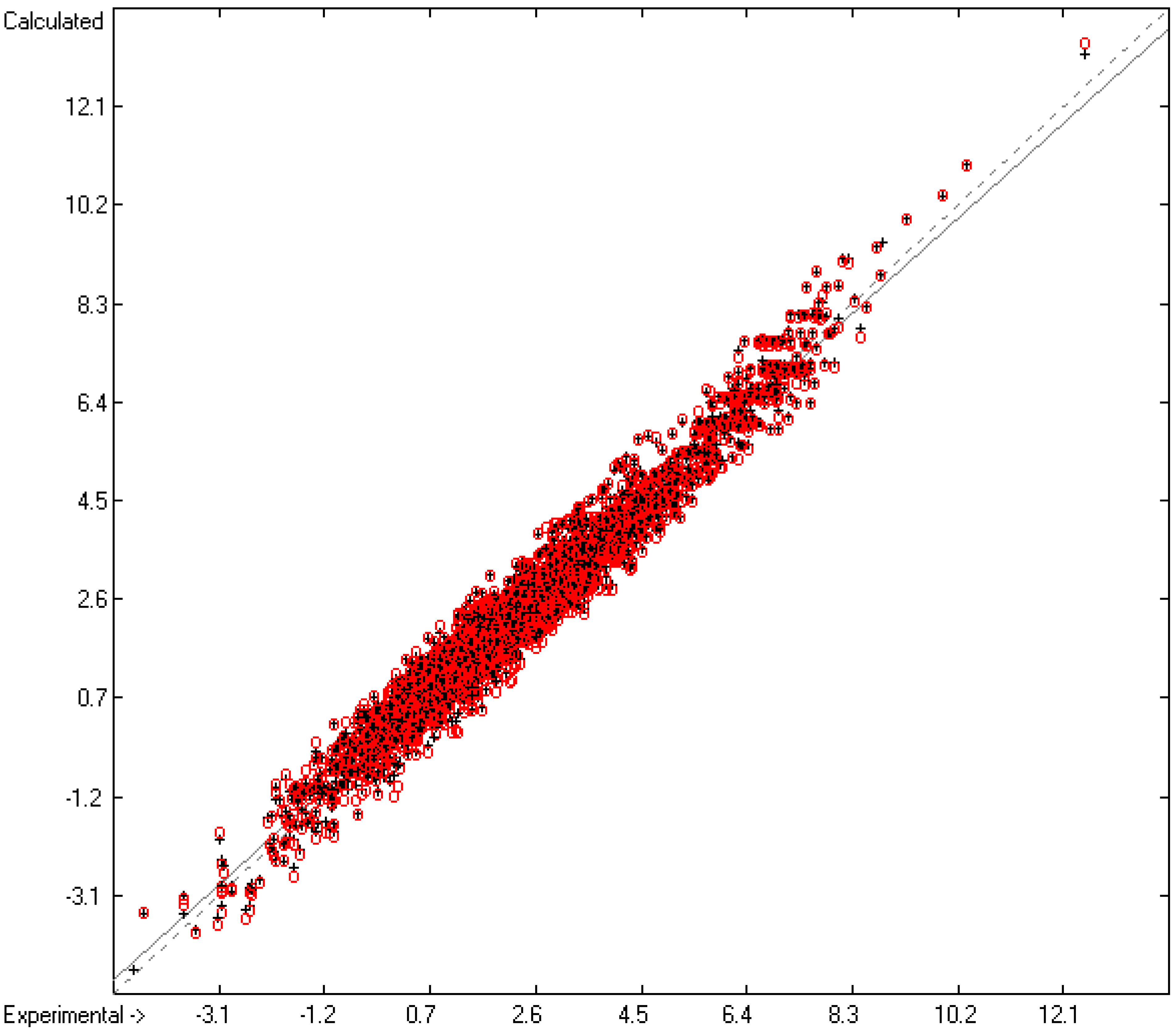
4.1. Partition Coefficient logP_ow

As shown at the bottom of Table 2, the number of molecules upon which the present group parameter set is based is 3332, substantially larger than the 2780 samples in our earlier paper [13]. Beyond this, the significantly better statistical results in Table 2 (lines B to H) with, e.g., a cross-validated (cv) standard deviation S of 0.42 (line H) vs. the earlier value of 0.51 is the result of the removal of molecules from the parameter computation for which the experimental value deviates by more than three times the value of S. The 122 molecules thus removed (3.5% of the total set) have been collected in an outlier list, available in the Supplementary Materials. The larger number of compounds for the group parameter computation not only significantly improved the statistical results but also enlarged the list of “valid” atom groups from 195 to 214, enabling the calculation of the logP_ow value of at present 29,462 molecules (79.4% of the total dataset). The correlation coefficients R² of 0.9648, the (cross-validated) Q² of 0.9599 and the cv standard error S of 0.42, based on 3246 and 3164 molecules, respectively, are significantly better than in our earlier paper [13] and compare very well not only with Klopman’s [8] results, which are based on a group-additivity method comparable to ours and have R² and Q² values of 0.93 and 0.926, respectively, but also with the statistical results of more elaborate calculation methods published recently [4,5,14,15,16]. As shown in the correlation diagram of Figure 2 and the histogram for Figure 3, the experimental logP_ow values range from −4.6 to +12.53 with a fairly even Gaussian error distribution.

Figure 2. Correlation diagram of the logP_ow data. Cross-validation data are superpositioned as red circles (10-fold cross-valid.: N = 3246; Q² = 0.9599; regression line: intercept = 0.1052; slope = 0.9636).

Figure 3. Histogram of the logP_ow data. Cross-validation data are superpositioned as red bars. (σ = 0.39; S = 0.42; experimental values range from −4.6 to +12.53).

It is worth mentioning that the observation discussed in our earlier paper (see Table 9 in [13]) concerning the two forms of amino acids (nonionic or zwitterionic) is not only confirmed by the new and extended group parameter set of Table 2 but also that the logP_ow differences in nearly all cases even more clearly distinguish the two forms. On the other hand, the ambiguous results concerning the keto/enol forms of the compounds listed in Table 10 in [13] could not be lifted by the new parameter set, which is not surprising in view of the sometimes strong solvent dependence of the equilibrium, as exemplified with acetylacetone [46]. In view of the discussion of certain particularities concerning the subsequent calculation of the third partition coefficient logK_aw in Section 4.3, it should be stressed at this point that the calculated logP_ow values for the hydrocarbons do not show any abnormal or systematic deviations from experimental values.

4.2. Partition Coefficient logK_oa

The calculation of the group parameter set of Table 3 used for the prediction of the logK_oa values is essentially based on the curated data set provided in Ebert’s paper [40], whereby compounds with just one “backbone atom” such as halomethanes or hydrocyanide had to be omitted as they are obviously not calculable using the present method. After the removal of another 129 compounds as outliers (6.36% of the total), following the same exclusion criterion as in the previous section, 1900 samples with their experimental data (line A in Table 3) remained for the computation of the group parameter values. Again, the outliers have been collected in a separate list available in the Supplementary Materials for readers who might want to re-evaluate their logK_oa values.

The subsequent calculation of the logK_oa values of 1829 training and 1765 test molecules based on 167 “valid” atom and special groups (line A) revealed excellent statistical results with a correlation coefficient R² of 0.9765, a standard deviation s of 0.44 (lines B and D) and a cross-validated Q² of 0.9717 with a corresponding S of 0.48 (lines F and H), visualised in the correlation diagram on Figure 4 and the histogram on Figure 5. These statistical data even outperform those given in Ebert’s paper and thus also the competing methods mentioned therein such as COSMOtherm [47] and EPI-Suite KOAWIN [48], not only confirming the versatility but also the reliability of the present group-additivity approach, which allowed the calculation of the logK_oa value for 27,044 molecules (72.9% of the entire database). Again, it should be kept in mind that just like in Section 4.1, any particularly large or systematic deviations between the experimental and calculated logK_oa values for the hydrocarbons could not be observed.

Figure 4. Correlation diagram of the logK_oa data. Cross-validation data are superpositioned as red circles (10-fold cross-valid.: N = 1829; Q² = 0.9717; regression line: intercept = 0.1997; slope = 0.9729; MAPD = 6.39%).

Figure 5. Histogram of the logK_oa data. Cross-validation data are superpositioned as red bars (σ = 0.44; S = 0.48; experimental values range from 0.28 to 17.15).

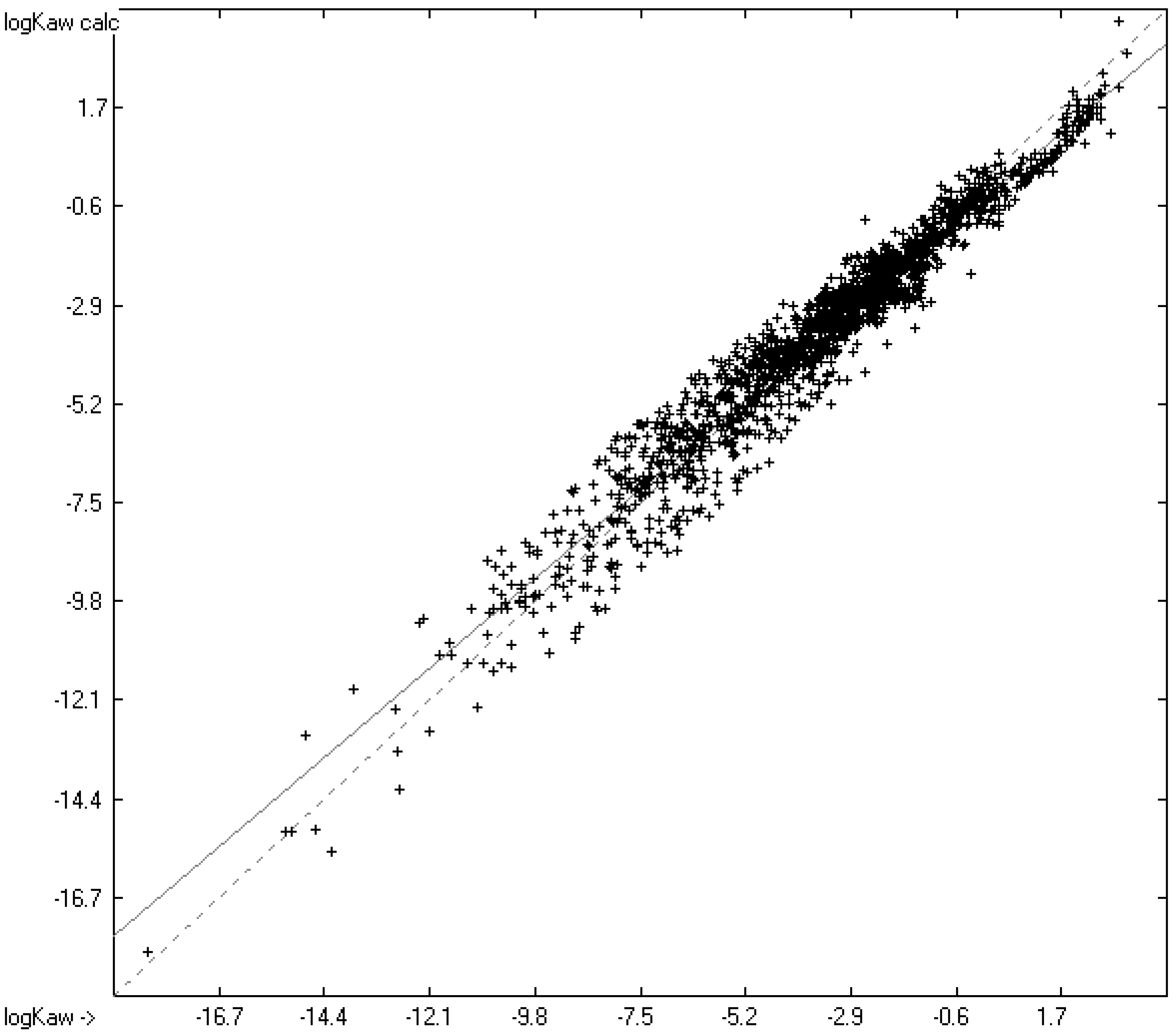
4.3. Partition Coefficient logK_aw

Once the partition coefficients logP_ow and logK_oa were calculated by means of the group-additivity method based on Table 2 and Table 3, respectively, it was easy to determine the logK_aw values, applying Equation (2) on each molecule in the database for which both descriptors had been calculated, adding up to 26,220 molecules. In order to assess the quality of the logK_aw values, it is important to recognise the flaws of this approach: while the logP_ow values were experimentally measured in a mixture of water-saturated octanol and octanol-saturated water, the logK_oa measurements occurred in dry octanol, an aspect that has been discussed in detail by Ebert et al. [40]. Hence, Equation (2) serves only as an approximation. In addition, since both descriptors on the right side of the equation appear with their own standard error, the error-propagation rule stipulates a standard error of logK_aw that is clearly larger than either of the two constituting descriptors. Entering the standard errors S for the test molecules of 0.42 (for logP_ow) and 0.48 (for logK_oa) into an error-propagation calculation, the expected standard error S for logK_aw is 0.638.

logK_aw (calc) = logP_ow (calc) − logK_oa (calc)

(2)

In order to test the reliability of the thus-calculated logK_aw values, a representative number of experimentally determined logK_aw data, extracted from the comprehensive databases of Ebert et al. [30] and Sander [45], were added to the database. In the latter case, the Henry’s law solubility constants H_s^cp were translated into the corresponding logK_aw values at 298.15 K. The comparison of the calculated with the experimental logK_aw values is visualised in the correlation diagram of Figure 6 and the histogram in Figure 7.

Figure 6. Correlation diagram of the logK_aw data (N = 1937; Q² = 0.9467; regression line: intercept = −0.4196; slope = 0.9044).

Figure 7. Histogram of the logK_aw data (S = 0.67; experimental values range from −17.99 to +3.71).

The complete set of experimental data was separated from the outliers, applying the same exclusion conditions as for the logP_ow and logK_oa values, and the outliers were collected in a corresponding list, available in the Supplementary Materials. Comparison of the remaining dataset with the calculated values yielded a standard error of 0.67, slightly higher than that predicted by the error-propagation calculation. A detailed analysis of the experimental data revealed two potential explanations for the inordinate scatter: (1) Within a series of substitution isomers, e.g., the tetra- or hexachlorobiphenyls, the tri- or pentachlorodiphenyl ethers or the dichloroanisoles, the experimental logK_aw values varied in a range of up to and over 1 unit, which was hard to assign to the specific positioning of the substituents. At any rate, the group-additivity-based calculation of the logP_ow and logK_oa values was not able to distinguish between these substitution isomers. (2) Sander’s comprehensive database of Henry’s law constants [45], listing the experimental H_s^cp values for a compound originating from various authors, showed for many compounds large differences between their H_s^cp values, in some cases exceeding one unit after translation into logK_aw, e.g., for undecane, acetylacetone or anthraquinone.

A thorough analysis of the correlation diagram in Figure 6 and the histogram in Figure 7 revealed an interesting peculiarity, visible as an indentation at the upper end of the correlation diagram and as a weak hump on the right side of the histogram: except for some siloxanes with experimental logK_aw values above 1.6 and normal scatter about calculated values, the predicted logK_aw for the remaining compounds with experimental logK_aw values above −1.0 were nearly systematically too low by ca. 0.5–1 units. It turned out that they were all pure hydrocarbons, in particular alkanes, alkenes and alkynes. The correlation diagram of the logK_aw data in Figure 8, focussing on these hydrocarbons, confirms this observation.

Figure 8. Correlation diagram of the logK_aw data for alkanes, alkenes and alkynes (N = 170).

Since, as mentioned in Section 4.1 and Section 4.2, no particularly large or systematic deviations between the experimental and calculated logP_ow and logK_oa data for the hydrocarbons could be detected, a potential explanation for this peculiarity might be based on the experimental conditions for the determination of the logP_ow values as mentioned by Ebert et al. [40]: since water-saturated octanol is a more polar solvent than pure octanol, while octanol-saturated water is less polar than pure water, the experimental logP_ow values, measured in an octanol/water mixture, tend to be shifted to smaller absolute values than theory would predict. While this is true for all measured solutes, it is possibly most effective for the least polar solutes such as the mentioned hydrocarbons, thus leading to experimental logP_ow values that are particularly low for the hydrocarbons. As a consequence, their calculation based on the group-additivity method predicts equally low logP_ow values, which again lead to low logK_aw data when Equation (2) is applied and when compared with experimental logK_aw values that are determined under pure air/water conditions.

4.4. Interpretation of the Special Groups’ Contributions to logP_ow and logK_oa, and Ultimately for logK_aw

While the atom group parameters are descriptor-specific and their comparison between descriptors does not make sense, special groups serve as differentiators of molecules that carry these groups from those that do not. Therefore, their meanings have overlapping descriptors; their values, however, must be viewed in the context of the value range of the descriptors. In the present case, the value ranges of logP_ow and logK_oa are similar (ca. 17 log units) and in the same area, and thus, a direct comparison of the special group contributions in Table 2 and Table 3 is permissible and leads to a few interesting observations: While the groups “(COH)n”, “Alkane”, “Unsaturated HC” and “Endocyclic bonds” in both tables only contribute to a minor degree (but nevertheless improve the statistical results) and consequently show only minor differences between the two tables, a significant difference was found for the groups “H/H Acceptor” and “(COOH)n”. The former special group, taking account of intramolecular hydrogen bridges, indicates a small but clearly higher chance of being a compound carrying an intramolecular H-bridge towards the octanol side in an octanol/water mixture, thus raising the logP_ow value. In contrast, the same H-bridge-carrying molecule has its inclination significantly shifted to the air side in an octanol/air environment compared to that without H-bridges, expressed in its lower logK_oa value. The reason may be found in the lower solvent–solute interaction caused by the H-bridge being bound intramolecularly, leading in both cases to a preference for the less polar of the respective two media. A typical example is the compound couple 2- and 3-nitroaniline, sampled in Table 5, where the former molecule carries a H-bridge between an amino-H and an oxygen of the nitro group.

Table 5. Experimental (calculated) logP_ow and logK_oa values of 2- and 3-nitroaniline.

An inverse effect can be found with molecules carrying two or more carboxylic acid functions: While the additional contribution of a second or third COOH function shows little effect in an octanol/water environment with a slightly increased shift towards water, leading to a lower logP_ow value, in an octanol/air environment, each additional COOH group drastically tilts the equilibrium towards the octanol side, thus strongly raising the logK_oa value. This may be demonstrated by the couple of hexanoic/1,6-hexanedioic acid, where both have the same carbon-chain length but where the second molecule carries two carboxylic acid functions, which tilts the octanol/air equilibrium by a factor of more than 10,000 towards the octanol side as shown in Table 6. Now, it is well known that monocarboxylic acids usually exist as dimeric associates in all three aggregate states. This association effect on the solubility is inherently taken into account in the atom group parameter evaluation of the COOH function. On the other hand, dicarboxylic acids do not only form dimers but also cyclical and linear oligomeric associates, with drastic consequences on their solubility in the various solvents. It is these additional associations that are considered by the special group “(COOH)n”.

Table 6. Experimental (calculated) logP_ow and logK_oa of hexanoic and 1,6-hexanedioic acid.

As a consequence, solutes with a low tendency to interact with solvents, either inherent or induced by intramolecular hydrogen bridges, show a trend to higher logK_aw values; the additional intermolecular association of di- and tricarboxylic acids, on the other hand, results in a significantly lower logK_aw value, as exemplified in Table 7, where the respective calculated data in Table 5 and Table 6 have been applied in Equation (2). The experimental logK_aw values have been extracted from Ebert et al. [30].

Table 7. Experimental and calculated logK_aw of some examples.

5. Conclusions

The present study, which is part of an ongoing project, put to use a tool for the simple and reliable calculation of the two partition coefficients logP_ow and logK_oa that has proven its unmatched versatility in the equally reliable prediction of now up to 19 physical, thermodynamic, solubility-, optics-, charge- and environment-related molecular descriptors [13,49,50,51,52,53,54,55], based on a common group-additivity method. The large database of more than 3300 and 1900 experimental data, respectively, upon which the group parameters for the logP_ow and logK_oa calculations are founded enabled their prediction for nearly 29,500 and more than 27,000 molecules, respectively, of the presently more than 37,100 compounds in ChemBrain’s database. In addition, these results also allowed the trustworthy calculation of the third partition coefficient logK_aw for more than 26,000 compounds. The big advantage of the present approach is its ease of use by simply adding, by means of paper and pencil, the parameters of the atoms and groups found in a particular molecule, which are listed in the respective Table 2 and Table 3.

The mentioned project’s software is called ChemBrain IXL, available from Neuronix Software, version ChemBrain IXL 5.9.70.1 (www.neuronix.ch (accessed on 27 November 2023), Rudolf Naef, Lupsingen, Switzerland).

Supplementary Materials

The following supporting information can be downloaded at https://www.mdpi.com/article/10.3390/liquids4010011/s1: The lists of compounds used in the present work, collected in their 3D structure together with their experimental data, are available as standard SDF files for use in external chemical software under the names of “S01. Compounds List for logPow-Parameters Calculations.sdf”, “S02. Compounds List for logKoa-Parameters Calculations.sdf” and “S03. Compounds List with exp logKaw Data”. The compounds used in the correlation diagrams and histograms are listed with their names and experimental and calculated data under the respective names of “S04. Compounds with Experimental vs. Calculated logPow Values.doc”, “S05. Compounds with Experimental vs. Calculated logKoa Values.doc”, “S06. Compounds with Experimental vs. Calculated logKaw Values.doc” and “S07. Alkanes, Alkenes and Alkynes with Exp. vs. Calc. logKaw Values.doc”. In addition, for each of the three partition coefficients, a list of their outliers has been added under the names of “S08. Outliers of logPow.doc”, “S09. Outliers of logKoa.doc” and “S10. Outliers of logKaw.doc”. Beyond this, the Supplementary Materials encompass all the figures and tables cited in the text as .tif and .doc files, respectively.

Author Contributions

R.N. developed the project ChemBrain and its software upon which this paper is based, and also fed the database, calculated and analysed the results and wrote the paper. W.E.A.J. suggested the extension of ChemBrain’s tool and contributed experimental data and the great majority of the literature references. Beyond this, R.N. is indebted to W.E.A.J. for the many valuable discussions. All authors have read and agreed to the published version of the manuscript.

Funding

This research received no external funding.

Data Availability Statement

The data presented in this study are available in the Supplementary Materials.

Acknowledgments

R.N. is indebted to the library of the University of Basel for allowing him full and free access to the electronic literature database.

Conflicts of Interest

The author declares no conflicts of interest.

References

Simonich, S.L.; Hites, R.A. Organic Pollutant Accumulation in Vegetation. Environ. Sci. Technol. 1995, 29, 2905–2914. [Google Scholar] [CrossRef]
McLachlan, M.S. Bioaccumulation of Hydrophobic Chemicals in Agricultural Food Chains. Environ. Sci. Technol. 1996, 30, 252–259. [Google Scholar] [CrossRef]
Doucette, W.J.; Shunthirsasingham, C.; Dettenmaier, E.M.; Zaleski, R.T.; Fantke, P.; Arnot, J.A. A Review of Measured Bioaccumulation Data on Terrestrial Plants for Organic Chemicals:Metrics, Variability, and the Need for Standardized Measurement Protocols. Environ. Toxicol. Chem. 2018, 37, 21–33. [Google Scholar] [CrossRef] [PubMed]
Nieto-Draghi, C.; Fayet, G.; Creton, B.; Rozanska, X.; Rotureau, P.; de Hemptinne, J.-C.; Ungerer, P.; Rousseau, B.; Adamo, C. A General Guidebook for the Theoretical Prediction of Physicochemical Properties of Chemicals for Regulatory Purposes. Chem. Rev. 2015, 115, 13093–13164. [Google Scholar] [CrossRef] [PubMed]
Cappelli, C.I.; Benfenati, E.; Cester, J. Evaluation of QSAR models for predicting the partition coefficient (log P) of chemicals under the REACH regulation. Environ. Res. 2015, 43, 26–32. [Google Scholar] [CrossRef]
Ghose, A.K.; Crippen, G.M. Atomic physicochemical parameters for three-dimensional structure-directed quantitative structure-activity relationships I. Partition coefficients as a measure of hydrophobicity. J. Computer. Chem. 1986, 7, 565–577. [Google Scholar] [CrossRef]
Ghose, A.K.; Pritchett, A.; Crippen, G.M. Atomic physicochemical parameters for three dimensional structure directed quantitative structure-activity relationships III: Modeling hydrophobic interactions. J. Comput. Chem. 1988, 9, 80–90. [Google Scholar] [CrossRef]
Klopman, G.; Li, J.-Y.; Wang, S.; Dimayuga, M. Computer automated log P calculations based on an extended group contribution approach. J. Chem. Inf. Comput. Sci. 1994, 34, 752–781. [Google Scholar] [CrossRef]
Visvanadhan, V.N.; Ghose, A.K.; Revankar, G.R.; Robins, R.K. Atomic physicochemical parameters for three dimensional structure directed quantitative structure-activity relationships. 4. Additional parameters for hydrophobic and dispersive interactions and their application for an automated superposition of certain naturally occurring nucleoside antibiotics. J. Chem. Inf. Comput. Sci. 1989, 29, 163–172. [Google Scholar] [CrossRef]
Leo, A.J. Calculating log P_oct from structures. Chem. Rev. 1993, 93, 1281–1306. [Google Scholar] [CrossRef]
Wang, R.; Fu, Y.; Lai, L. A new atom-additive method for calculating partition coefficients. J. Chem. Inf. Comput. Sci. 1997, 37, 615–621. [Google Scholar] [CrossRef]
Hou, T.J.; Xu, X.J. ADME evaluation in drug discovery. 2. Prediction of partition coefficient by atom-additive approach based on atom-weighted solvent accessible surface areas. J. Chem. Inf. Comput. Sci. 2003, 43, 1058–1067. [Google Scholar] [CrossRef]
Naef, R. A Generally Applicable Computer Algorithm Based on the Group Additivity Method for the Calculation of Seven Molecular Descriptors: Heat of Combustion, LogP_O/W, LogS, Refractivity, Polarizability, Toxicity and LogBB of Organic Compounds; Scope and Limits of Applicability. Molecules 2015, 20, 18279–18351. [Google Scholar] [CrossRef] [PubMed]
Plante, J.; Werner, S. JPlogP: An improved logP predictor trained using predicted data. J. Cheminform. 2018, 10, 61. [Google Scholar] [CrossRef] [PubMed]
Ulrich, N.; Goss, K.-U.; Ebert, A. Exploring the octanol–water partition coefficient dataset using deep learning techniques and data augmentation. Com. Chem. 2021, 4, 90. [Google Scholar] [CrossRef] [PubMed]
Sun, Y.; Hou, T.; He, X.; Man, V.H.; Wang, J. Development and test of highly accurate endpoint free energy methods. 2: Prediction of logarithm of n-octanol–water partition coefficient (logP) for druglike molecules using MM-PBSA method. J. Comput. Chem. 2023, 44, 1300–1311. [Google Scholar] [CrossRef] [PubMed]
Chen, J.; Harner, T.; Schramm, K.W.; Quan, X.; Xue, X.; Wu, W.; Kettrup, A. Quantitative relationships between molecular structures, environmental temperatures and octanol/air partition coefficients of PCDD/Fs. Sci. Total Environ. 2002, 300, 155–166. [Google Scholar] [CrossRef] [PubMed]
Chen, J.; Harner, T.; Yang, P.; Quan, X.; Chen, S.; Schramm, K.W.; Kettrup, A. Quantitative predictive models for octanol/air partition coefficients of polybrominated diphenyl ethers at different temperatures. Chemosphere 2003, 51, 577–584. [Google Scholar] [CrossRef] [PubMed]
Chen, J.; Harner, T.; Schramm, K.W.; Quan, X.; Xue, X.; Kettrup, A. Quantitative relationships between molecular structures, environmental temperatures and octanol/air partition coefficients of polychlorinated biphenyls. Comput. Biol. Chem. 2003, 27, 405–421. [Google Scholar] [CrossRef]
Zhao, H.; Chen, J.; Quan, X.; Qu, B.; Liang, X. Octanol/air partition coefficients of polybrominated biphenyls. Chemosphere 2009, 74, 1490–1494. [Google Scholar] [CrossRef]
Staikova, M.; Wania, F.; Donaldson, D. Molecular polarizability as a single parameter predictor of vapour pressures and octanoleair partitioning coefficients of non-polar compounds: A priori approach and results. Atmos. Environ. 2004, 38, 213–225. [Google Scholar] [CrossRef]
Zhao, H.; Zhang, Q.; Chen, J.; Xue, X.; Liang, X. Prediction of octanol/air partition coefficients of semivolatile organic compounds based on molecular connectivity index. Chemosphere 2005, 59, 1421–1426. [Google Scholar] [CrossRef]
Zeng, X.L.; Zhang, X.L.; Wang, Y. Qspr modeling of n-octanol/air partition coefficients and liquid vapor pressures of polychlorinated dibenzo-p-dioxins. Chemosphere 2013, 91, 229–232. [Google Scholar] [CrossRef] [PubMed]
Liu, H.; Shi, J.; Liu, H.; Wang, Z. Improved 3D-QSPR analysis of the predictive octanol/air partition coefficients of hydroxylated and methoxylated polybrominated diphenyl ethers. Atmos. Environ. 2013, 77, 840–845. [Google Scholar] [CrossRef]
Jiao, L.; Gao, M.; Wang, X.; Li, H. QSPR study on the octanol/air partition coefficient of polybrominated diphenyl ethers by using molecular distance-edge vector index. Chem. Cent. J. 2014, 8, 36. [Google Scholar] [CrossRef][Green Version]
Chen, Y.; Cai, X.; Jiang, L.; Li, Y. Prediction of octanol-air partition coefficients for polychlorinated biphenyls (PCBs) using 3D-SQAR models. Ecotoxicol. Environ. Saf. 2016, 124, 202–212. [Google Scholar] [CrossRef] [PubMed]
Fu, Z.; Chen, J.; Li, X.; Wang, Y.; Yu, H. Comparison of prediction methods for octanol-air partition coefficients of diverse organic compounds. Chemosphere 2016, 148, 118–125. [Google Scholar] [CrossRef] [PubMed]
Jin, X.; Fu, Z.; Li, X.; Chen, J. Development of polyparameter linear free energy relationship models for octanol/air partition coefficients of diverse chemicals. Environ. Sci. Process. Impact. 2017, 19, 300–306. [Google Scholar] [CrossRef] [PubMed]
Li, X.; Chen, J.; Zhang, L.; Qiao, X.; Huang, L. The fragment constant method for predicting octanol/air partition coefficients of persistent organic pollutants at different temperatures. J. Phys. Chem. Ref. Data 2006, 35, 1365–1384. [Google Scholar] [CrossRef]
Ebert, R.-U.; Kühne, R.; Schüürmann, G. Henry’s Law Constant—A General-Purpose Fragment Model to Predict Log Kaw from Molecular Structure. Environ. Sci. Technol. 2023, 57, 160–167. [Google Scholar] [CrossRef]
Hardtwig, E. Fehler—Und Ausgleichsrechnung; Bibliographisches Institut AG: Mannheim, Germany, 1968. [Google Scholar]
Sangster, J. Octanol-water partition coefficients of simple organic compounds. J. Phys. Chem. Ref. Data 1989, 18, 1111–1229. [Google Scholar] [CrossRef]
Lipinski, C.A.; Lombardo, F.; Dominy, B.W.; Feeney, P.J. Experimental and computational approaches to estimate solubility and permeability in drug discovery and development settings. Adv. Drug Deliv. Rev. 1997, 23, 3–25. [Google Scholar] [CrossRef]
Tewari, Y.B.; Miller, M.M.; St. Wasik, P.; Martire, D.E. Aqueous Solubility and Octanol/Water Partition Coefficient of Organic Compounds at 25.0 °C. J. Chem. Eng. Data 1982, 27, 451–454. [Google Scholar] [CrossRef]
Abraham, M.H.; Chadha, H.S.; Whiting, G.S.; Mitchell, R.C. Hydrogen Bonding. 32. An Analysis of Water-Octanol and Water-Alkane Partitioning and the Δlog P Parameter of Seiler. J. Pharm. Sci. 1994, 83, 1085–1100. [Google Scholar] [CrossRef] [PubMed]
St. Czerwinski, E.; Skvorak, J.P.; Maxwell, D.M.; Lenz, D.E.; St. Baskin, I. Organophosphorus Compounds on Biodistribution and Percutaneous Toxicity. J. Biochem. Mol. Tox. 2006, 20, 241–246. [Google Scholar] [CrossRef] [PubMed]
Boddu, V.M.; Abburi, K.; St. Maloney, W.; Damavarapu, R. Thermophysical Properties of an Insensitive Munitions Compound, 2,4-Dinitroanisole. J. Chem. Eng. Data 2008, 53, 1120–1125. [Google Scholar] [CrossRef]
Li, X.-J.; Shan, G.; Liu, H.; Wang, Z.-Y. Determination of lgK_ow and QSPR Study on Some Fluorobenzene Derivatives. Chin. J. Struct. Chem. 2009, 28, 1236–1241. [Google Scholar]
Saranjampour, P.; Vebrosky, E.N.; Armbrust, K.L. Salinity Impacts on Water Solubility and n-Octanol/Water Partition Coefficients of Selected Pesticides and Oil Constituents. Environ. Toxicol. Chem. 2017, 36, 2274–2280. [Google Scholar] [CrossRef] [PubMed]
Ebert, R.-U.; Kühne, R.; Schüürmann, G. Octanol/Air Partition Coefficient. A General-Purpose Fragment Model to Predict Log Koa from Molecular Structure. Environ. Sci. Technol. 2023, 57, 976–984. [Google Scholar] [CrossRef] [PubMed]
Puzyn, T.; Falandysz, J.; Rostkowski, P.; Piliszek, S.; Wilczynska, A. Computational estimation of logarithm of octanol/air partition coefficients and subcooled vapour pressures for each of 75 chloronaphtalene congeners. Phys.-Chem. Prop. Distr. Model. Organohal. Compds. 2004, 66, 2354–2360. [Google Scholar] [CrossRef]
Odabasi, M.; Cetin, E.; Sofuoglu, A. Determination of octanol–air partition coefficients and supercooled liquid vapor pressures of PAHs as a function of temperature: Application to gas–particle partitioning in an urban atmosphere. Atm. Environ. 2006, 40, 6615–6625. [Google Scholar] [CrossRef]
Xu, S.; Kropscott, B. Method for Simultaneous Determination of Partition Coefficients for Cyclic Volatile Methylsiloxanes and Dimethylsilanediol. Anal. Chem. 2012, 84, 1948–1955. [Google Scholar] [CrossRef] [PubMed]
Easterbrook, K.D.; Vona, M.A.; Osthoff, H.D. Measurement of Henry’s law constants of ethyl nitrate in deionized water, synthetic sea salt solutions, and n-octanol. Chemosphere 2024, 346, 140482. [Google Scholar] [CrossRef] [PubMed]
Sander, R. Compilation of Henry’s law constants (version 5.0.0) for water as solvent. Atmos. Chem. Phys. 2023, 23, 10901–12440. [Google Scholar] [CrossRef]
Allen, G.; Dwek, R.A. An n.m.r. study of keto-enol tautomerism in β-diketones. J. Chem. Soc. B 1966, 1966, 161–163. [Google Scholar] [CrossRef]
COSMOlogic GmbH Co. KG. A Dassault Systemes Company, Version 19.0.4, COSMOthermX. 2019. Available online: www.cosmologic.de (accessed on 4 December 2023).
US EPA. Estimation Programs Interface Suite for Microsoft Windows; Version 4.11, Module KOAWIN v. 1.11; United States Environmental Protection Agency: Washington, DC, USA, 2015. [Google Scholar]
Naef, R.; Acree, W.E., Jr. Calculation of Five Thermodynamic Molecular Descriptors by Means of a General Computer Algorithm Based on the Group-Additivity Method: Standard Enthalpies of Vaporization, Sublimation and Solvation, and Entropy of Fusion of Ordinary Organic Molecules and Total Phase-Change Entropy of Liquid Crystals. Molecules 2017, 22, 1059. [Google Scholar] [CrossRef]
Naef, R.; Acree, W.E. Application of a General Computer Algorithm Based on the Group-Additivity Method for the Calculation of Two Molecular Descriptors at Both Ends of Dilution: Liquid Viscosity and Activity Coefficient inWater at Infinite Dilution. Molecules 2018, 23, 5. [Google Scholar] [CrossRef]
Naef, R.; Acree, W.E., Jr. Calculation of the Surface Tension of Ordinary Organic and Ionic Liquids by Means of a Generally Applicable Computer Algorithm Based on the Group-Additivity Method. Molecules 2018, 23, 1224. [Google Scholar] [CrossRef] [PubMed]
Naef, R. Calculation of the Isobaric Heat Capacities of the Liquid and Solid Phase of Organic Compounds at 298.15K by Means of the Group-Additivity Method. Molecules 2020, 25, 1147. [Google Scholar] [CrossRef]
Naef, R.; Acree, W.E., Jr. Calculation of the Vapour Pressure of Organic Molecules by Means of a Group-Additivity Method and Their Resultant Gibbs Free Energy and Entropy of Vaporization at 298.15 K. Molecules 2021, 26, 1045. [Google Scholar] [CrossRef] [PubMed]
Naef, R.; Acree, W.E., Jr. Revision and Extension of a Generally Applicable Group-Additivity Method for the Calculation of the Standard Heat of Combustion and Formation of Organic Molecules. Molecules 2021, 26, 6101. [Google Scholar] [CrossRef] [PubMed]
Naef, R.; Acree, W.E., Jr. Revision and Extension of a Generally Applicable Group Additivity Method for the Calculation of the Refractivity and Polarizability of Organic Molecules at 298.15 K. Liquids 2022, 2, 327–377. [Google Scholar] [CrossRef]

Figure 1. Endosulfan sulphate (graphics by ChemBrain IXL).

Figure 2. Correlation diagram of the logP_ow data. Cross-validation data are superpositioned as red circles (10-fold cross-valid.: N = 3246; Q² = 0.9599; regression line: intercept = 0.1052; slope = 0.9636).

Figure 3. Histogram of the logP_ow data. Cross-validation data are superpositioned as red bars. (σ = 0.39; S = 0.42; experimental values range from −4.6 to +12.53).

Figure 4. Correlation diagram of the logK_oa data. Cross-validation data are superpositioned as red circles (10-fold cross-valid.: N = 1829; Q² = 0.9717; regression line: intercept = 0.1997; slope = 0.9729; MAPD = 6.39%).

Figure 5. Histogram of the logK_oa data. Cross-validation data are superpositioned as red bars (σ = 0.44; S = 0.48; experimental values range from 0.28 to 17.15).

Figure 6. Correlation diagram of the logK_aw data (N = 1937; Q² = 0.9467; regression line: intercept = −0.4196; slope = 0.9044).

Figure 7. Histogram of the logK_aw data (S = 0.67; experimental values range from −17.99 to +3.71).

Figure 8. Correlation diagram of the logK_aw data for alkanes, alkenes and alkynes (N = 170).

Table 1. Special groups and their meaning.

Atom Type	Neighbours	Meaning
H	H Acceptor	Correction value for intramolecular H bridge between acidic H (on O, N or S) and basic acceptor (O, N or F)
(COH)n	n > 1	Correction value for each additional hydroxy group
(COOH)n	n > 1	Correction value for each additional carboxylic acid group
Alkane	No. of C atoms	Correction value for each C atom in a pure alkane
Unsaturated HC	No. of C atoms	Correction value for each C atom in an aromatic hydrocarbon
Endocyclic bonds	No. of single bonds	Correction value for each single endocyclic bond

Table 2. Atom and special groups and their contribution in logP_ow calculations.

Entry	Atom Type	Neighbours	Contribution	Occurrences	Molecules
1	Const		0.73	3332	3332
2	B(−)	F4	2.71	10	10
3	C sp3	H3C	0.27	2614	1498
4	C sp3	H3N	0.14	457	320
5	C sp3	H3N(+)	−1.35	2	2
6	C sp3	H3O	−0.26	375	285
7	C sp3	H3P	−0.3	4	4
8	C sp3	H3S	−0.34	61	53
9	C sp3	H3Si	0.76	44	5
10	C sp3	H2C2	0.44	3262	1046
11	C sp3	H2CN	0.42	741	429
12	C sp3	H2CN(+)	−0.86	32	25
13	C sp3	H2CO	−0.1	799	604
14	C sp3	H2CS	−0.33	97	69
15	C sp3	H2CF	−0.29	5	5
16	C sp3	H2CCl	0.33	84	67
17	C sp3	H2CBr	0.41	54	48
18	C sp3	H2CJ	1.08	6	6
19	C sp3	H2CP	2.77	1	1
20	C sp3	H2N2	2.05	3	3
21	C sp3	H2NO	0.46	4	4
22	C sp3	H2NS	0.72	3	3
23	C sp3	H2O2	−0.17	6	6
24	C sp3	H2S2	−0.86	6	6
25	C sp3	HC3	0.45	417	269
26	C sp3	HC2N	0.58	200	157
27	C sp3	HC2N(+)	−0.73	25	24
28	C sp3	HC2O	0.1	383	241
29	C sp3	HC2S	−0.21	8	8
30	C sp3	HC2F	−0.36	2	2
31	C sp3	HC2Cl	0.69	64	22
32	C sp3	HC2Br	0.81	26	22
33	C sp3	HCN2	1.2	6	5
34	C sp3	HCNO	1.15	17	17
35	C sp3	HCNS	0.9	25	25
36	C sp3	HCO2	−0.02	31	22
37	C sp3	HCOS	0.6	3	3
38	C sp3	HCOCl	0.19	3	1
39	C sp3	HCOBr	1.03	1	1
40	C sp3	HCOP	0.31	1	1
41	C sp3	HCF2	−0.02	2	2
42	C sp3	HCCl2	0.93	13	12
43	C sp3	HOF2	−0.04	1	1
44	C sp3	C4	0.54	144	111
45	C sp3	C3N	0.71	37	36
46	C sp3	C3N(+)	−0.43	6	6
47	C sp3	C3O	0.04	54	52
48	C sp3	C3S	−0.1	17	17
49	C sp3	C3F	0.94	4	4
50	C sp3	C3Cl	0.8	21	8
51	C sp3	C3Br	0.59	5	4
52	C sp3	C2N2	−1.17	1	1
53	C sp3	C2NO	0.52	5	5
54	C sp3	C2O2	1.65	5	5
55	C sp3	C2F2	0.67	2	2
56	C sp3	C2Cl2	0.84	9	9
57	C sp3	CNO2	1.46	1	1
58	C sp3	CF3	0.86	80	76
59	C sp3	CF2Cl	1.1	3	2
60	C sp3	CFCl2	1.1	3	2
61	C sp3	CCl3	1.6	23	21
62	C sp3	CCl2Br	0	1	1
63	C sp3	CBr3	2.44	1	1
64	C sp3	OF3	0.8	2	2
65	C sp3	SF3	1.04	8	8
66	C sp3	SFCl2	1.9	1	1
67	C sp3	SCl3	0.76	3	3
68	C sp2	H2=C	0.25	97	87
69	C sp2	H2=N	−0.62	1	1
70	C sp2	HC=C	0.24	449	285
71	C sp2	HC=N	−1.98	18	18
72	C sp2	HC=N(+)	0.94	10	10
73	C sp2	H=CN	−0.08	146	109
74	C sp2	H=CN(+)	−0.6	18	18
75	C sp2	HC=O	−0.73	45	45
76	C sp2	H=CO	0.32	14	13
77	C sp2	H=CS	0.02	17	16
78	C sp2	H=CCl	0.51	8	6
79	C sp2	H=CBr	0.59	1	1
80	C sp2	HN=N	−0.06	65	52
81	C sp2	HN=O	−0.63	16	15
82	C sp2	HO=O	−0.4	10	10
83	C sp2	H=NS	−0.51	4	4
84	C sp2	C2=C	0.38	160	133
85	C sp2	C2=N	−0.25	105	102
86	C sp2	C2=N(+)	2.45	1	1
87	C sp2	C2=O	−0.86	242	194
88	C sp2	C=CN	0.76	76	64
89	C sp2	C=CN(+)	−0.56	3	3
90	C sp2	C=CO	0.64	41	36
91	C sp2	C=CS	−0.16	17	15
92	C sp2	C=CF	−0.01	3	3
93	C sp2	C=CCl	0.81	31	21
94	C sp2	C=CBr	0.94	4	4
95	C sp2	C=CJ	0.89	1	1
96	C sp2	C=CP	0	1	1
97	C sp2	=CN2	1.36	19	19
98	C sp2	=CN2(+)	0.74	11	11
99	C sp2	CN=N	0.24	67	63
100	C sp2	CN=N(+)	−0.67	1	1
101	C sp2	CN=O	−0.69	449	364
102	C sp2	C=NO	−0.76	1	1
103	C sp2	=CNO	−0.01	4	4
104	C sp2	=CNO(+)	−0.37	2	2
105	C sp2	CN=S	−0.36	8	8
106	C sp2	C=NS	0.07	5	4
107	C sp2	=CNS	0.37	4	4
108	C sp2	=CNCl	1.94	1	1
109	C sp2	=CNBr	0.7	5	3
110	C sp2	C=NCl	1.75	1	1
111	C sp2	CO=O	−0.13	700	613
112	C sp2	CO=O(-)	−2.16	35	35
113	C sp2	C=OS	−0.99	4	4
114	C sp2	C=OCl	0.28	4	4
115	C sp2	=COCl	1.27	1	1
116	C sp2	=CS2	0	3	3
117	C sp2	=CSBr	−2.41	1	1
118	C sp2	=CF2	0.26	1	1
119	C sp2	=CCl2	1.21	12	10
120	C sp2	=CBr2	1.36	1	1
121	C sp2	N2=N	0.79	26	25
122	C sp2	N2=N(+)	0.74	1	1
123	C sp2	N2=O	0.07	135	134
124	C sp2	N=NO	0.11	1	1
125	C sp2	N2=S	0.11	9	8
126	C sp2	N=NS	0.24	25	24
127	C sp2	N=NCl	1.13	3	3
128	C sp2	N=NBr	0.24	3	2
129	C sp2	NO=O	0.2	117	114
130	C sp2	=NOS	−0.19	1	1
131	C sp2	N=OS	0.05	7	7
132	C sp2	NO=S	0.97	1	1
133	C sp2	=NS2	−1.65	2	2
134	C sp2	NS=S	−1.02	5	3
135	C sp2	=NSCl	1.17	1	1
136	C sp2	O2=O	0	3	3
137	C sp2	O=OCl	−0.13	3	3
138	C aromatic	H:C2	0.25	9963	2133
139	C aromatic	H:C:N	−0.49	283	193
140	C aromatic	H:C:N(+)	0.22	33	27
141	C aromatic	H:N2	−0.91	9	9
142	C aromatic	:C3	0.25	389	170
143	C aromatic	C:C2	0.32	2023	1351
144	C aromatic	C:C:N	−0.38	74	62
145	C aromatic	C:C:N(+)	−3.29	4	3
146	C aromatic	:C2N	0.39	653	534
147	C aromatic	:C2N(+)	−0.15	194	161
148	C aromatic	:C2:N	−0.09	93	72
149	C aromatic	:C2:N(+)	−3.54	19	19
150	C aromatic	:C2O	0.57	1076	742
151	C aromatic	:C2S	0.08	208	170
152	C aromatic	:C2F	0.27	126	86
153	C aromatic	:C2Cl	0.78	1718	565
154	C aromatic	:C2Br	0.9	248	111
155	C aromatic	:C2J	1.26	50	34
156	C aromatic	:C2P	1.08	1	1
157	C aromatic	C:N2	−1.81	9	9
158	C aromatic	:C:N2	−0.13	1	1
159	C aromatic	:CN:N	0.49	38	34
160	C aromatic	:CN:N(+)	−0.83	1	1
161	C aromatic	:C:NO	0.97	21	15
162	C aromatic	:C:NS	−0.16	5	5
163	C aromatic	:C:NF	−0.23	4	3
164	C aromatic	:C:NCl	0.16	18	16
165	C aromatic	:C:NBr	0.06	1	1
166	C aromatic	N:N2	−0.05	51	41
167	C aromatic	N:N2(+)	0	1	1
168	C aromatic	:N2O	1.53	8	8
169	C aromatic	:N2S	0.8	3	3
170	C aromatic	:N2Cl	0.89	6	6
171	C(+) aromatic	H:N2	0.21	25	25
172	C sp	H#C	−0.27	28	28
173	C sp	C#C	0.2	86	57
174	C sp	C#N	−0.7	136	130
175	C sp	N#N	0.04	3	3
176	C sp	#NS	−0.59	5	5
177	C sp	=N=O	0.64	4	4
178	C sp	=N=S	1.53	27	26
179	N sp3	H2C	−1.57	86	84
180	N sp3	H2C(pi)	−1.05	326	292
181	N sp3	H2N	−0.85	20	20
182	N sp3	H2S	−1.55	34	34
183	N sp3	HC2	−1.3	74	73
184	N sp3	HC2(pi)	−0.93	225	203
185	N sp3	HC2(2pi)	−0.47	311	272
186	N sp3	HCN	−1.1	4	3
187	N sp3	HCN(pi)	−0.49	14	13
188	N sp3	HCN(2pi)	1.65	42	42
189	N sp3	HCO(pi)	−1.32	9	9
190	N sp3	HCS	−1.69	4	4
191	N sp3	HCS(pi)	−0.98	47	47
192	N sp3	HCP	−1.78	3	3
193	N sp3	HCP(pi)	−0.41	1	1
194	N sp3	C3	−1.03	122	108
195	N sp3	C3(pi)	−0.73	153	138
196	N sp3	C3(2pi)	−0.72	149	136
197	N sp3	C3(3pi)	−0.75	23	23
198	N sp3	C2N	−1.57	1	1
199	N sp3	C2N(pi)	−1.41	31	28
200	N sp3	C2N(2pi)	−0.67	51	47
201	N sp3	C2N(3pi)	−0.44	10	10
202	N sp3	C2O(pi)	−0.31	5	5
203	N sp3	C2S	−1.42	5	5
204	N sp3	C2S(pi)	0.03	7	6
205	N sp3	C2S(2pi)	0.76	2	2
206	N sp3	C2P	−0.33	5	3
207	N sp3	CN2(2pi)	1.36	1	1
208	N sp3	CS2	0.27	1	1
209	N sp3	CS2(pi)	−0.29	1	1
210	N sp2	H=C	−0.67	12	11
211	N sp2	C=C	−0.72	200	180
212	N sp2	C=N	0.01	13	12
213	N sp2	=CN	0.49	96	78
214	N sp2	C=N(+)	−6.61	1	1
215	N sp2	=CN(+)	−1.02	2	2
216	N sp2	=CO	−0.64	47	41
217	N sp2	C=O	−1.05	2	2
218	N sp2	=CS	−1.44	5	4
219	N sp2	N=N	−0.78	25	18
220	N sp2	N=O	0.16	40	37
221	N aromatic	C2:C(+)	0	50	25
222	N aromatic	:C2	0.38	354	258
223	N aromatic	:C:N	−0.35	4	2
224	N(+) sp3	H3C	−1.03	26	26
225	N(+) sp3	H2C2	1.2	5	5
226	N(+) sp3	HC3	2.68	1	1
227	N(+) sp3	C4	3.03	1	1
228	N(+) sp2	C=CO(−)	−2.3	10	10
229	N(+) sp2	CO=O(−)	0.27	235	198
230	N(+) sp2	NO=O(−)	−0.19	2	2
231	N(+) sp2	O2=O(−)	0.44	55	29
232	N(+) aromatic	H:C2	2.5	3	3
233	N(+) aromatic	C:C2	−0.48	7	6
234	N(+) aromatic	:C2O(−)	1.73	19	19
235	N(+) sp	=C=N(−)	1.8	1	1
236	N(+) sp	=N2(−)	0	1	1
237	O	HC	−0.96	481	344
238	O	HC(pi)	−0.72	627	557
239	O	HN	−0.15	11	11
240	O	HN(pi)	−0.24	6	6
241	O	C2	0.06	156	115
242	O	C2(pi)	−0.13	726	588
243	O	C2(2pi)	−0.51	301	280
244	O	CN	0.4	3	3
245	O	CN(pi)	0.82	4	4
246	O	CN(+)(pi)	0.01	55	29
247	O	CN(2pi)	0.53	13	12
248	O	CS	−0.13	13	8
249	O	CS(pi)	−0.1	3	3
250	O	CP	0.23	132	68
251	O	CP(pi)	−0.49	36	26
252	O	CSi	−0.15	8	2
253	O	N2(2pi)	1.91	5	5
254	O	NP(pi)	−1.95	14	14
255	O	Si2	0.09	18	4
256	S2	HC	0.65	14	12
257	S2	HC(pi)	0.14	31	31
258	S2	C2	1.39	48	45
259	S2	C2(pi)	0.98	68	63
260	S2	C2(2pi)	0.98	55	54
261	S2	CN	0	3	3
262	S2	CN(2pi)	2.3	1	1
263	S2	CS	0.87	2	1
264	S2	CS(pi)	1.97	4	2
265	S2	CP	1.12	17	15
266	S2	CP(pi)	0.48	3	2
267	S2	N2	−2.2	2	2
268	S2	N2(2pi)	5.96	1	1
269	S4	C2=O	−1.13	11	11
270	S4	C2=O2	−0.5	16	16
271	S4	CO=O2	−0.48	2	1
272	S4	CN=O2	−0.05	85	80
273	S4	C=O2F	0.24	2	2
274	S4	NO=O2	0	3	3
275	S4	N2=O2	0.77	5	5
276	S4	O2=O	0.83	2	2
277	S4	O2=O2	0.5	2	2
278	S4	O2=O2(−)	−1.14	3	3
279	P4	CO2=O	−1.11	2	2
280	P4	CO2=S	0.26	1	1
281	P4	CO=OS	−2.58	1	1
282	P4	CO=OF	−0.88	3	3
283	P4	COS=S	−2.04	1	1
284	P4	O3=O	−0.56	29	29
285	P4	O3=S	1.12	18	18
286	P4	O2S=S	0.7	12	11
287	P4	O=OS2	−0.54	2	2
288	P4	N3=O	−0.31	1	1
289	P4	N2O=O	0.24	2	2
290	P4	NO=OS	−1.5	2	2
291	Si	C4	−0.51	1	1
292	Si	C3O	−1.7	2	1
293	Si	C2O2	0.13	17	4
294	Si	O4	0	2	2
295	Halide		1.1	20	19
296	H	H Acceptor	0.51	164	154
297	(COH)n	n > 1	0.26	137	74
298	(COOH)n	n > 1	−0.15	26	25
299	Alkane	No. of C atoms	0.09	290	32
300	Unsaturated HC	No. of C atoms	0.02	1584	135
301	Endocyclic bonds	No. of single bds	−0.14	2338	384
A	Based on	Valid groups	214		3332
B	Goodness of fit	R²	0.9648		3246
C	Deviation	Average	0.31		3246
D	Deviation	Standard	0.39		3246
E	K-fold cv	K	10		3164
F	Goodness of fit	Q²	0.9599		3164
G	Deviation	Average (cv)	0.33		3164
H	Deviation	Standard (cv)	0.42		3164

Table 3. Atom and special groups and their contribution in logK_oa calculations.

Entry	Atom Type	Neighbours	Contribution	Occurrences	Molecules
1	Const		1.46	1900	1900
2	C sp3	H3C	−0.07	1800	875
3	C sp3	H3N	3.42	131	87
4	C sp3	H3N(+)	1.42	1	1
5	C sp3	H3O	2.24	292	219
6	C sp3	H3S	1.51	30	26
7	C sp3	H3P	−0.42	3	3
8	C sp3	H3Si	0.42	68	11
9	C sp3	H2C2	0.43	1732	538
10	C sp3	H2CN	3.91	191	129
11	C sp3	H2CN(+)	1.64	6	5
12	C sp3	H2CO	2.61	535	342
13	C sp3	H2CS	1.76	57	44
14	C sp3	H2CP	2.58	3	3
15	C sp3	H2CF	−0.77	3	3
16	C sp3	H2CCl	0.71	75	56
17	C sp3	H2CBr	1.05	23	18
18	C sp3	H2CJ	1.13	5	5
19	C sp3	H2CSi	2.91	4	4
20	C sp3	H2N2	4.89	8	3
21	C sp3	H2NO	5.65	9	8
22	C sp3	H2NS	4.67	5	5
23	C sp3	H2O2	4.78	6	4
24	C sp3	H2S2	3.74	4	4
25	C sp3	HC3	0.64	268	180
26	C sp3	HC2N	4.08	64	53
27	C sp3	HC2N(+)	2.05	1	1
28	C sp3	HC2O	2.86	169	135
29	C sp3	HC2S	1.76	9	7
30	C sp3	HC2F	−1.66	1	1
31	C sp3	HC2Cl	1.21	43	17
32	C sp3	HC2Br	1.31	14	9
33	C sp3	HC2J	1.95	1	1
34	C sp3	HCNO	8.18	3	3
35	C sp3	HCNS	2.08	1	1
36	C sp3	HCO2	5.73	6	6
37	C sp3	HCF2	−0.18	7	7
38	C sp3	HCFCl	0.02	2	2
39	C sp3	HCCl2	1.18	15	14
40	C sp3	HCClBr	0.77	1	1
41	C sp3	HOF2	1.79	3	3
42	C sp3	C4	0.73	98	84
43	C sp3	C3N	4.1	13	13
44	C sp3	C3O	3.11	40	37
45	C sp3	C3S	2.6	3	3
46	C sp3	C3Cl	0.87	37	15
47	C sp3	C2NO	5.94	1	1
48	C sp3	C2O2	5.94	6	6
49	C sp3	C2F2	0.23	58	10
50	C sp3	C2Cl2	1.24	18	17
51	C sp3	CNO2	9.56	1	1
52	C sp3	COF2	3.06	3	3
53	C sp3	CF3	−0.06	55	51
54	C sp3	CF2Cl	−0.02	4	3
55	C sp3	CFCl2	0.37	3	2
56	C sp3	CCl3	1.62	17	16
57	C sp3	CBr3	0.57	1	1
58	C sp3	O2F2	6.85	1	1
59	C sp3	OF3	1.86	3	3
60	C sp2	H2=C	−0.19	88	76
61	C sp2	HC=C	0.34	233	141
62	C sp2	HC=N	0.85	8	8
63	C sp2	HC=O	1	27	27
64	C sp2	H=CN	1.1	19	13
65	C sp2	H=CO	0.48	15	14
66	C sp2	H=CS	−1.08	9	7
67	C sp2	H=CCl	0.44	12	10
68	C sp2	H=CBr	0.6	3	2
69	C sp2	H=CSi	2.17	1	1
70	C sp2	HN=N	1.73	53	30
71	C sp2	HN=O	2.27	3	3
72	C sp2	HO=O	0.92	4	4
73	C sp2	H=NS	2.88	1	1
74	C sp2	C2=C	0.8	103	79
75	C sp2	C2=N	1.62	34	30
76	C sp2	C=CN	1.6	19	16
77	C sp2	C2=O	1.08	87	75
78	C sp2	C=CO	1.22	27	26
79	C sp2	C=CP	−0.09	1	1
80	C sp2	C=CS	−0.41	14	10
81	C sp2	C=CCl	0.62	39	24
82	C sp2	C=CBr	1.01	12	5
83	C sp2	=CN2	2.98	2	2
84	C sp2	CN=N	2.75	7	7
85	C sp2	CN=O	2.64	93	88
86	C sp2	C=NO	1.26	5	5
87	C sp2	=CNO	−1.24	3	3
88	C sp2	C=NS	0.46	6	6
89	C sp2	=CNCl	3.35	6	3
90	C sp2	CO=O	1.73	244	210
91	C sp2	C=OS	−0.61	3	2
92	C sp2	=CS2	−0.66	1	1
93	C sp2	=CF2	−1.14	1	1
94	C sp2	=CCl2	1.14	16	14
95	C sp2	N2=N	3.36	9	9
96	C sp2	N2=O	3.65	43	40
97	C sp2	N=NO	2.64	4	4
98	C sp2	N=NS	0.71	7	7
99	C sp2	NO=O	2.81	38	36
100	C sp2	N=OS	0.93	17	17
101	C sp2	NO=S	4.26	1	1
102	C sp2	=NOS	0.68	3	3
103	C sp2	NS=S	6.03	3	2
104	C sp2	=NSCl	−5.44	2	2
105	C sp2	O2=O	2.56	3	3
106	C aromatic	H:C2	0.31	5436	1136
107	C aromatic	H:C:N	0.53	81	49
108	C aromatic	H:N2	0.17	6	6
109	C aromatic	:C3	0.89	441	148
110	C aromatic	C:C2	0.79	1163	657
111	C aromatic	C:C:N	0.68	42	30
112	C aromatic	:C2N	1.35	164	146
113	C aromatic	:C2N(+)	2.09	96	69
114	C aromatic	:C2:N	1.01	13	10
115	C aromatic	:C2O	1.27	769	453
116	C aromatic	:C2P	3.53	5	3
117	C aromatic	:C2S	−0.19	38	33
118	C aromatic	:C2Si	−0.25	1	1
119	C aromatic	:C2F	0.13	99	41
120	C aromatic	:C2Cl	0.91	1844	550
121	C aromatic	:C2Br	1.24	391	143
122	C aromatic	:C2J	2.14	10	9
123	C aromatic	C:N2	0.77	11	10
124	C aromatic	:CN:N	0.8	4	4
125	C aromatic	:C:NO	1.2	28	24
126	C aromatic	:C:NCl	0.9	14	12
127	C aromatic	N:N2	1.18	60	36
128	C aromatic	:N2O	1.15	11	11
129	C aromatic	:N2S	−0.6	8	8
130	C aromatic	:N2Cl	0.43	9	8
131	C sp	H#C	−0.45	18	17
132	C sp	C#C	0.67	18	17
133	C sp	C#N	0.73	46	43
134	C sp	N#N	5.32	1	1
135	C sp	#NP	−5.58	1	1
136	C sp	=N=S	−0.13	2	2
137	N sp3	H2C	−2.18	17	16
138	N sp3	H2C(pi)	1.02	57	53
139	N sp3	H2N	3.57	5	5
140	N sp3	H2S	1.81	1	1
141	N sp3	HC2	−5.94	12	11
142	N sp3	HC2(pi)	−2.38	93	70
143	N sp3	HC2(2pi)	0.08	65	56
144	N sp3	HCN(pi)	0.02	5	4
145	N sp3	HCN(2pi)	1.2	4	4
146	N sp3	HCO(pi)	1.13	1	1
147	N sp3	HCP	−4.1	3	3
148	N sp3	HCP(pi)	1.51	1	1
149	N sp3	HCS(pi)	−1.54	8	8
150	N sp3	C3	−9.44	17	17
151	N sp3	C3(pi)	−6.39	58	55
152	N sp3	C3(2pi)	−4.82	49	45
153	N sp3	C3(3pi)	−3.61	9	9
154	N sp3	C2N	−5.12	1	1
155	N sp3	C2N(pi)	−2.54	15	14
156	N sp3	C2N(+)(pi)	−1.93	7	2
157	N sp3	C2N(2pi)	−3.84	36	36
158	N sp3	C2N(3pi)	−0.65	13	12
159	N sp3	C2P	0	1	1
160	N sp3	C2P(pi)	−2.97	1	1
161	N sp3	C2P(2pi)	−4.07	1	1
162	N sp2	H=C	0.51	1	1
163	N sp2	C=C	−0.97	54	48
164	N sp2	C=N	0.61	6	4
165	N sp2	=CN	0.03	54	49
166	N sp2	=CN(+)	9.74	2	2
167	N sp2	=CO	−3.65	30	26
168	N sp2	N=N	−1.3	4	3
169	N sp2	N=O	−2.02	13	13
170	N aromatic	:C2	0.54	194	109
171	N aromatic	:C:N	0.47	4	1
172	N(+) sp2	CO=O(−)	−0.36	104	76
173	N(+) sp2	NO=O(−)	0	9	4
174	N(+) sp2	O2=O(−)	−1.09	63	35
175	O	HC	−0.66	143	121
176	O	HC(pi)	1.39	175	159
177	O	HN(pi)	4.18	2	2
178	O	HP	2.11	4	2
179	O	HSi	1.91	3	2
180	O	C2	−4.17	139	105
181	O	C2(pi)	−2.68	392	317
182	O	C2(2pi)	−0.92	255	228
183	O	CN(pi)	0.51	20	16
184	O	CN(+)(pi)	0.1	63	35
185	O	CN(2pi)	3.07	8	8
186	O	CO(pi)	−1.03	2	1
187	O	CS	−0.88	11	6
188	O	CP	−1.2	183	93
189	O	CP(pi)	−0.01	70	54
190	O	CSi	−2.38	9	3
191	O	NP(pi)	4.65	1	1
192	O	P2	1.7	1	1
193	O	Si2	0	21	6
194	P4	C3=O	−5.7	1	1
195	P4	CNO=O	1.2	1	1
196	P4	CO2=O	1.47	3	3
197	P4	CO2=S	−1.5	3	3
198	P4	CO=OS	1.99	1	1
199	P4	CO=OF	1.94	1	1
200	P4	COS=S	−0.86	1	1
201	P4	NO2=O	3.42	1	1
202	P4	NO2=S	1.88	3	3
203	P4	NO=OS	1.2	2	2
204	P4	O3=O	0.09	29	29
205	P4	O3=S	−0.4	32	30
206	P4	O2=OS	0.43	5	5
207	P4	O2=OF	−0.17	1	1
208	P4	O=OS2	1.58	3	3
209	P4	O2S=S	−0.27	18	17
210	P4	=OS3	1.46	1	1
211	S2	HC	−1.08	2	2
212	S2	HC(pi)	1.54	1	1
213	S2	C2	−1.5	14	14
214	S2	C2(pi)	0.4	41	39
215	S2	C2(2pi)	2.82	24	23
216	S2	CS	−0.58	4	2
217	S2	CS(pi)	−2.98	2	1
218	S2	CP	−0.12	33	28
219	S2	CP(pi)	1.78	3	2
220	S4	C2=O	0.6	2	2
221	S4	C2=O2	2.13	3	3
222	S4	CN=O2	3.26	9	9
223	S4	CO=O2	−0.05	1	1
224	S4	O2=O	−0.35	2	2
225	S4	O2=O2	0.24	3	3
226	S6	CF5	1.92	3	3
227	Si	C4	−1.33	3	3
228	Si	C3O	−0.65	7	4
229	Si	C2O2	0.1	19	6
230	Si	CO3	0	3	3
231	H	H Acceptor	−1.51	47	45
232	(COH)n	n > 1	0.06	22	15
233	(COOH)n	n > 1	1.2	6	6
234	Alkane	No. of C atoms	−0.05	268	34
235	Unsaturated HC	No. of C atoms	−0.03	1512	140
236	Endocyclic bonds	No. of single bds	−0.11	1109	210
A	Based on	Valid groups	167		1900
B	Goodness of fit	R²	0.9765		1829
C	Deviation	Average	0.34		1829
D	Deviation	Standard	0.44		1829
E	K-fold cv	K	10		1765
F	Goodness of fit	Q²	0.9717		1765
G	Deviation	Average (cv)	0.37		1765
H	Deviation	Standard (cv)	0.48		1765

Table 4. Example calculation of the logK_oa of endosulfan sulphate.

Atom Type	C sp3	C sp3	C sp3	C sp3	C sp2	O	S4	Endocycl. Bonds	Const	Sum
Neighbors	H2CO	HC3	C3Cl	C2Cl2	C=CCl	CS	O2=O2	n C-C
Contribution	2.61	0.64	0.87	1.24	0.62	−0.88	0.24	−0.11	1.46
n Groups	2	2	2	1	2	2	1	9
n × Contribution	5.22	1.28	1.74	1.24	1.24	−1.76	0.24	−0.99	1.46	9.67

Table 5. Experimental (calculated) logP_ow and logK_oa values of 2- and 3-nitroaniline.

Descriptor	2-Nitroaniline	3-Nitroaniline
logP_ow	1.85 (1.70)	1.37 (1.19)
logK_oa	6.46 (5.29)	7.62 (6.80)

Table 6. Experimental (calculated) logP_ow and logK_oa of hexanoic and 1,6-hexanedioic acid.

Descriptor	Hexanoic Acid	1,6-Hexanedioic Acid
logP_ow	1.92 (1.91)	0.08 (0.64)
logK_oa	6.31 (6.23)	10.74 (10.62)

Table 7. Experimental and calculated logK_aw of some examples.

Compound	logK_aw Exp	logK_aw Calc
2-Nitroaniline	−4.77	−3.59
3-Nitroaniline	−6.49	−5.61
Hexanoic Acid	−4.531	−4.32
1,6-Hexanedioic Acid	−11.15	−9.98

Disclaimer/Publisher’s Note: The statements, opinions and data contained in all publications are solely those of the individual author(s) and contributor(s) and not of MDPI and/or the editor(s). MDPI and/or the editor(s) disclaim responsibility for any injury to people or property resulting from any ideas, methods, instructions or products referred to in the content.

© 2024 by the authors. Licensee MDPI, Basel, Switzerland. This article is an open access article distributed under the terms and conditions of the Creative Commons Attribution (CC BY) license (https://creativecommons.org/licenses/by/4.0/).

Calculation of the Three Partition Coefficients logP_ow, logK_oa and logK_aw of Organic Molecules at Standard Conditions at Once by Means of a Generally Applicable Group-Additivity Method

Abstract

1. Introduction

2. Method

2.1. Definition of the Atom and Special Groups

2.2. Calculation of the Atom and Special Group Contributions