Abstract
A computational model that can accurately describe the thermodynamics of a hydrocarbon system and its properties under various conditions is a prerequisite for running reservoir and pipeline simulations. Cubic Equations of State (EoS) are mathematical tools used to model the phase and volumetric behavior of reservoir fluids when compositional effects need to be considered. To anticipate uncertainty and enhance the quality of their predictions, EoS models must be adjusted to adequately match the available lab-measured PVT values. This task is challenging given that there are many potential tuning parameters, thus leading to various tuning results of questionable validity. In this paper, we present an automated EoS tuning workflow that employs a Generalized Pattern Search (GPS) optimizer for efficient tuning of a cubic EoS model. Specifically, we focus on the Peng–Robinson (PR) model, which is the oil and gas industry standard, to accurately capture the behavior of diverse multicomponent, complex hydrocarbon mixtures encountered in subsurface reservoirs. This approach surpasses the limitations of conventional gradient-based (GB) methods, which are susceptible to getting trapped in local optima. The proposed technique also allows physical constraints to be imposed on the optimization procedure. A gas condensate and an H2S-rich oil were used to demonstrate the effectiveness of the GPS algorithm in finding an optimized solution for high-dimensional search spaces, and its superiority over conventional gradient-based optimization was confirmed by automatically tracking globally optimal and physically sound solutions.
1. Introduction
When conducting flow simulations in petroleum engineering, fluid properties play a vital role in all types of calculations, including the estimation of recoverable reserves, the analysis of fluid flow within reservoirs and wellbores, the design of surface pipeline systems, and the selection of processing equipment. Phase behavior, pressure–volume–temperature (PVT) values, rheology, and thermal properties are all incorporated into the governing differential equations that impose the principles of mass, momentum, and energy conservation. Consequently, these factors have a direct impact on production forecasts and optimization processes. Among these factors, PVT values hold particular importance as they describe the changes in volume and physical properties that occur during fluid depletion and flash processes [1], which take place during production through wellbores and surface separation systems.
The sampling process for petroleum fluids is fundamental in the development of reservoirs as subsequent standard and routine PVT analyses deliver valuable data regarding the phase and volumetric behavior of reservoir fluids [2]. Due to the economically unattractive cost of the laboratory experiments included in main PVT analyses [3,4], these are performed on specific condition paths imposed by the reservoir itself [4]. On account of limited experimental data, a computational model is required to predict a fluid’s behavior under a wide range of conditions expected to be encountered during the exploitation of a field.
Simplistic models based on the black oil principle satisfactorily describe hydrocarbon fluids when the oil and gas phases maintain a fixed overall composition throughout production [5]. However, in cases where the displacement process depends on both pressure and fluid composition, black oil models are unable to capture the thermodynamic effects taking place. Many field development projects exhibit strong composition dependence, among them, volatile oil or gas condensate reservoir depletion, miscible gas injection for oil reservoirs, and liquid recovery under lean gas injection for gas condensate reservoirs [6]. In these cases, all hydrocarbon phases should be treated as nc-component mixtures and thus a compositional model should be utilized instead [7].
The most commonly used compositional models for hydrocarbon systems and their mixtures are cubic Equations of State (cEoS), such as the Peng–Robinson (PR) [8,9] and Soave–Redlich–Kwong (SRK) [10] fluid models, which are among the most computationally efficient cEoS [11]. In general, an EoS model requires properties that define the vapor pressure curve of each individual component present in the hydrocarbon mixture under study: the critical pressure (Pc), critical temperature (Tc), acentric factor (ω), and binary interaction coefficients (BICs or kijs) [12]. In addition, properties that ensure accurate predictions of the liquid density of each fluid component are also a prerequisite, such as the molecular weight (MW) and volume translation (Vs) parameter [12].
However, EoS cannot be used directly as predictive models [13] due to their relatively simplistic semi-empirical approach to physical phenomena [14], their inherent deficiencies in estimating liquid density, and the uncertainties in the molecular weight and critical properties of the pseudo-components [4]. These shortcomings render EoS insufficient for accurately simulating the phase and volumetric behavior of reservoir fluids under various conditions.
The standard approach to overcoming these challenges is to tune the adjustable EoS parameters against available experimental data [14]. The optimal values of the selected regressing components parameters are obtained as soon as the error function, defined by the difference between the predicted and the lab measured PVT values, is minimized. Over the years, numerous tuning techniques have been proposed, the majority of which typically begin with assigning default values to the components of properties and the characterization of the plus fraction followed by the minimization of the error function using gradient-based (GB) optimizers.
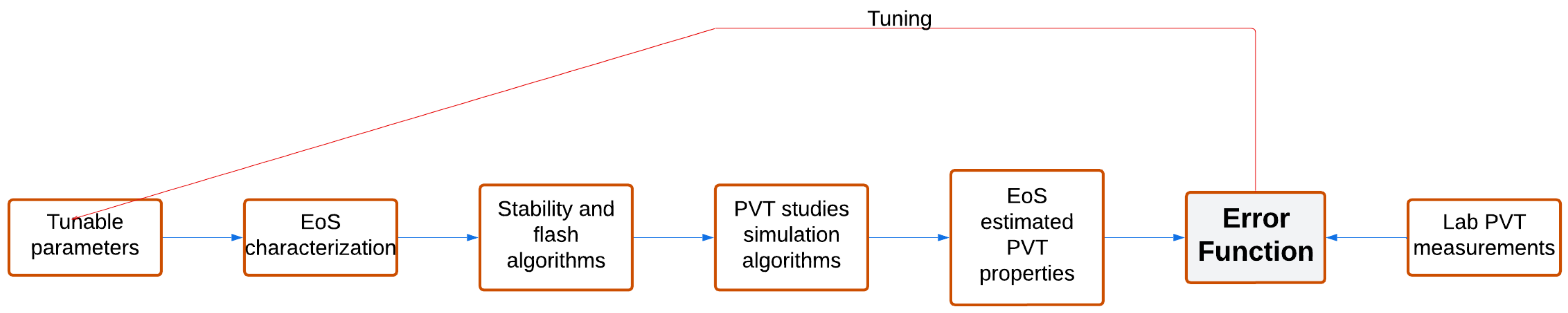
Figure 1 describes graphically the EoS tuning process. This process is mathematically complicated; at the same time, it requires careful inspection of the physical interpretation of the values assigned to each tuned parameter. In other words, it is vital to pay particular attention to the physical soundness of the values attributed to the regression parameters apart from attempting to minimize the global error.
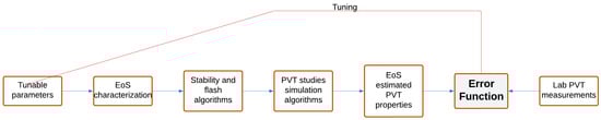
Figure 1.
EoS tuning process.
Due to the significant number of matching parameters, EoS tuning is undoubtedly a challenging task that depends to a great extent on the operator’s experience. For this reason, although many operators have developed ‘‘best practices’’ and EoS tuning workflows, they still rely on the services of experienced fluid engineers, when it comes to complex fluids. In addition, the strong nonlinearity of the error function (i.e., between the PVT values and the tunable parameters) makes the EoS tuning problem even more complex. Things become even more complicated when an EoS model needs to be simultaneously tuned against more than one reservoir fluid as is the case when commingled flow is considered. Therefore, it is reasonable to consider the implementation of global optimization techniques to obtain a reliable EoS model because of their wider viewing angle with regard to seeking the global minimum. To this end, Sarvestani et al. [15] and Zarifi et al. [16] conducted research on EoS tuning using global optimization in the form of genetic algorithms (GAs) [15,16]. In both of their studies, commercial PVT software programs, which use Newton’s numerical method as an optimization technique, have been coupled with GAs to further assess the software output and modify the selected EoS parameters.
Regarding research to ensure physically sound EoS tuning, various investigators have proposed simplistic approaches such as incorporating box constraints to define limits for regression parameters as part of their tuning methodologies. Among the most well-known methodologies are those proposed by Coats and Smart [17], Christensen [18], and Aguilar and McCain [19].
The proposed methodology in this paper, being fully automated and directly incorporable into any related software, offers three main advantages. Firstly, it utilizes a Generalized Pattern Search (GPS) algorithm (global optimization technique) for handling the EoS tuning problem, which acts as a compromise between the fully random, exhaustively time-consuming GAs and the much faster, but prone to be trapped in local minima, gradient-based (GB) methods. Secondly, the tuning algorithm developed in this work is flexible and allows a number of mathematical constraints to be imposed on the optimization process to account for all physics-driven rules a reasonably tuned EoS model needs to honor, rather than solely simplistic box constraints. This introduces an additional layer of reliability and accuracy to the tuned EoS model ensuring not only that the attained minimum will be the global one but that it will not “twist” the EoS model to such an extent that unrealistic behavior is predicted by the tuned model. Finally, the proposed methodology being fully automated addresses the challenge of achieving accurate EoS tuning with minimal operator dependence.
The rest of this paper is organized as follows. Section 2 describes the standard workflow followed in the oil and gas industry for developing a compositional model. Section 3 provides a comprehensive discussion of EoS tuning, which constitutes the central theme and primary objective of this work. Section 4 and Section 5 present the physical constraints imposed and the features of GPS algorithms, respectively. Finally, the new automated EoS tuning algorithm developed and the results from the test application of the proposed methodology are presented in Section 6. The paper concludes in Section 7.
2. Best Practices for Developing a Compositional Model
During the development of a compositional simulation model, engineers aim at keeping the number of components low to reduce CPU time and memory usage during the simulations which will follow. Nevertheless, the model’s efficiency in providing accurate predictions tends to worsen as the number of components decreases. Clearly, reaching an optimal lumped EoS model that maintains the accuracy of the split model is not an easy task. Therefore, during the development of compositional models for pilot or full-scale flow simulations, standard practices can be followed.
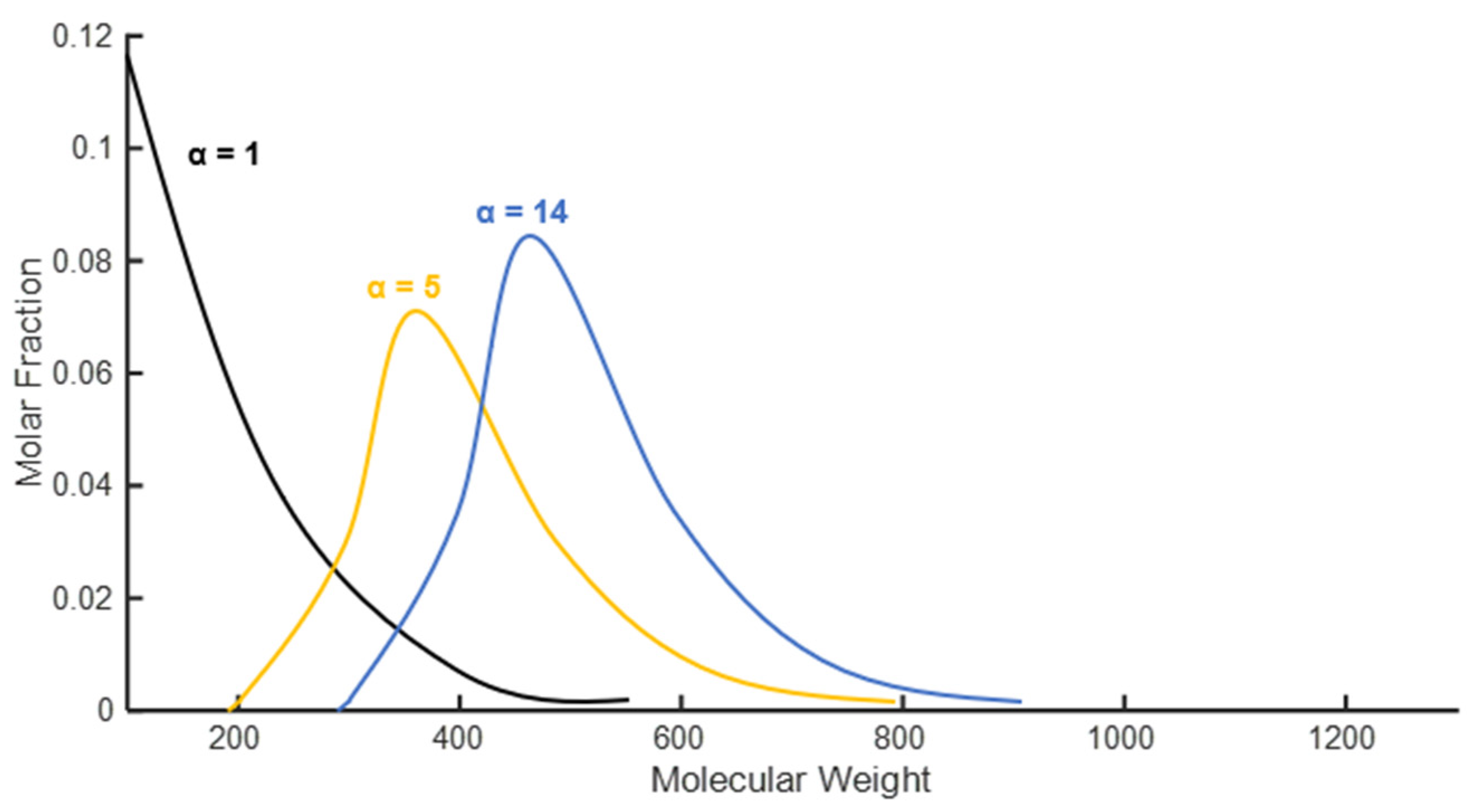
The first step towards developing an EoS model is to mathematically split the plus fraction into several single carbon number (SCN) fractions using either Pedersen’s splitting scheme [20], in which an exponential relationship is assumed between mole fractions and the molecular weight of SCN, or the generalized three-parameter gamma probability function developed by Whitson [21]. In the context of the gamma distribution, parameter α plays a vital role in shaping the distribution’s form, as exemplified in Figure 2, which provides a visual representation of how the gamma distribution model relates the SCN mole fraction to SCN molecular weight. When it comes to reservoir fluids, this parameter typically ranges from 0.5 to 2.5, with higher values corresponding to heavier fluids and lower values indicating lighter fluids. It is important to note that when α equals to 1, the gamma distribution reduces to an exponential distribution. Based on the resulting split model, a pseudoized EoS is developed for modeling calculations to be carried out within a reasonable time.
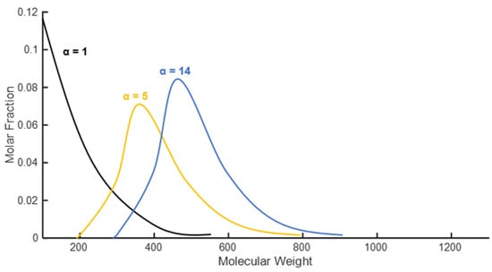
Figure 2.
Gamma distributions for petroleum residues.
The next step incorporates the grouping of similar components into pseudo-ones to keep the total number of components as low as possible. Typically, light and pure components such as methane (C1), ethane (C2), and propane (C3) are grouped with nitrogen (N2), carbon dioxide (CO2), and hydrogen sulfide (H2S), respectively; the isomers of butane (i-C4 and n-C4) and pentane (i-C5 and n-C5) are grouped into a single pseudo-component or two separate ones. When N2, CO2, or H2S content exceeds approximately 2% in the reservoir fluid or injection gas, these components are recommended to be kept intact. The properties and BICs of the resulting pseudo-components can be determined using a mixing rule since pseudoization is considered as a process of “combining streams” [22]. Finally, the numerous SCN fractions must be lumped into few multiple carbon number (MCN) components using Whitson’s method, for instance. This lumping method makes use of mixing rules and is embedded in the majority of PVT software packages which are integral components of commercial reservoir simulators. The obtained lumped pseudos are then characterized using empirical correlations, which are functions of their molecular weight and specific gravity. BICs of the HCs-HCs binary systems can be defined by the Prausnitz correlation [23].
Adjustments to the component and pseudo-component properties to match the measured PVT data can occur during the tuning of the EoS model. However, due to the excessive flexibility of the optimization process involved, EoS tuning is advised to be performed in a stepwise manner; matching saturation pressures and PVT properties should be attempted each time a new grouping scheme is evaluated.
3. Tuning of EoS Models
The objective of EoS tuning against laboratory measurements for a specific reservoir fluid is to achieve the highest level of accuracy and precision in describing the phase behavior and physical properties of hydrocarbon mixtures with an EoS model. It should be emphasized that there is no universal solution when it comes to EoS tuning, as the tuning process must be customized to align with the objectives and limitations of each individual field development project under study.
The EoS tuning process involves solving an optimization problem to minimize the error function, which is a key element during EoS calibration as it allows engineers to quantitatively assess the accuracy of their models. The error function J is usually defined as the sum of the weighted squared relative deviations between the laboratory measurements and the EoS estimates:
where and correspond to the calculated and experimental PVT values, respectively. Weights , which are associated with single pressure steps or groups of steps, assign a degree of importance to each data point. Box constraints are typically applied to avoid unrealistic adjustable parameters values. For bounding values of each tunable variable, it is generally accepted to allow a variation within the range of ±20% for the Pc, Tc, ω, and Vs of each component, as well as ±0.05 for the BICs [24].
Calibrating an EoS model is intrinsically challenging due to the strong nonlinearity that governs Equation (1), thus rendering it as a nonlinear optimization problem involving complicated relationships between the variables being optimized. Furthermore, compositional models require the adjustment of a large number of EoS parameters to provide high-quality predictions, which makes EoS tuning a high-dimensional optimization problem. Solving this type of optimization problem is particularly difficult because of the ‘‘curse of dimensionality’’ which implies that the size of the search domain increases exponentially with the number of parameters. The high dimensionality of the EoS tuning optimization problem results in Equation (1) having numerous local optima, which can trap optimization algorithms and impede their ability to reach global optimum. This risk is particularly high when utilizing gradient-based (GB) optimizers. To mitigate the risk of being trapped in a local minimum, it is typical to run GB optimizers repeatedly using different initial estimates.
Tuning a compositional model poses the additional challenge of determining appropriate weighting factors, which play a crucial role in extrapolation—the use of the tuned EoS model to predict a fluid’s behavior under conditions beyond those for which experimental data are available. It is important to note that each modification of the assigned weighting factors leads to the complete alteration of the shape of the error function (Equation (1)); minima and maxima appear or vanish when compared with optimization problems, where different sets of weighting factors are used.
To assign weighting factors to each property, one must assess the relative importance of key data, account for the amount of data for a specific PVT property, and consider the uncertainty associated with the available laboratory data, to lend confidence to the ability of the tuned EoS model to provide reliable estimations. However, this procedure is highly subjective and closely linked to the level of experience of the operator performing the EoS tuning.
The general approach is to appoint the highest weighting factors to saturation pressures since they represent the state at which vapor and liquid are in equilibrium, and they are fewer in number than other data types, such as densities and relative oil volumes. Furthermore, high weights are assigned to thermodynamic properties that are especially significant in the application of interest. Additionally, Constant Composition Expansion (CCE) volume versus pressure data typically receive high weights during tuning due to their elevated reliability, attributed to the fact that no mass removal occurs during the CCE experiment, as opposed to other conventional PVT tests. Finally, when there is a significant difference in magnitude between the PVT properties, greater weight is assigned to the property with the lower magnitude to ensure a balanced and reliable model calibration.
Finally, accurately predicting fluid behavior across a wide range of pressures and temperatures, including high and low values, is a further hurdle of EoS tuning. In particular, the challenge lies in matching both the surface and reservoir properties [12], which often proves significantly challenging for GB optimizers.
4. Tuning Constraints
The preceding discussion highlights the need to use an optimizer designed to search the entire solution space to attain global solutions. However, even with a global optimizer and box constraints, physically sound-tuned EoS models cannot be guaranteed. Therefore, the imposition of advanced thermodynamic constraints in addition to the box ones is necessary to ensure the validity and accuracy of the resulting EoS models.
To maintain the hierarchy of component properties during the EoS tuning process, it is essential to implement inequality constraints which ensure that, as SCN increases, key thermodynamic properties such as Tc, ω, Vs, and BICs or kijs exhibit corresponding increases, whereas Pc decreases. These constraints map to the following inequalities:
where corresponds to the SCN.
Alternatively, the pseudos’ properties can be forced to lie within the range defined by the lightest and the heaviest component in the MCN group. For a group MCNi-j spanning SCNs from to , the following inequalities must hold:
The molar mass of the pseudos is often tuned to match density measurements by directly affecting the mass contained in the molar volume. In such case, the pseudos’ molar mass values should be modified under the constraint that the heavy end molar mass is honored, that is:
where index rolls over all pseudos comprising the heavy end. It should be noted that the heavy end molar mass is calculated by mass balance utilizing the STO molar mass which has been measured by Freezing Point Depression (FPD) or Vapor Pressure Osmometry (VPO). Although the experimental error in either method may be non-negligible, this error is attenuated when limited to that considered in the Cn+ heavy end, thus justifying the use of Equation (4). However, the popularity of adjusting the molecular weights has declined in recent years, as the introduction of volume shift parameters has been found to adequately enhance the accuracy of density predictions. Similarly to the molar mass, heavy end density should be honored as well by requiring that the volume additivity is retained, i.e.,
A more complex set of constraints can also be envisaged following the work presented by Gaganis et al. in [25]. Such constraints impose the necessity of PVT properties’ derivatives with respect to components concentration rather than the properties themselves or the adjustable parameters, to follow specific patterns or to exhibit a specific sign. Derivatives such as are defined by considering the change in the PVT property (e.g., ) when increasing the concentration of some component while subtracting an equal number of moles distributed proportionally from all remaining components. For example, whenever the amount of a pseudo increases, against all other components, PVT properties accounting for the volatility of the reservoir fluid should be reducing whereas properties such as density should increase. In fact, the heavier the component considered, the greater is expected to be the effect on the PVT properties’ derivatives.
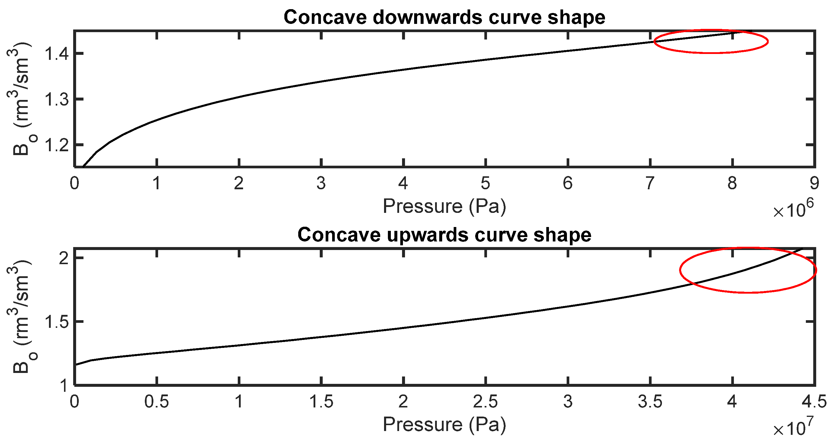
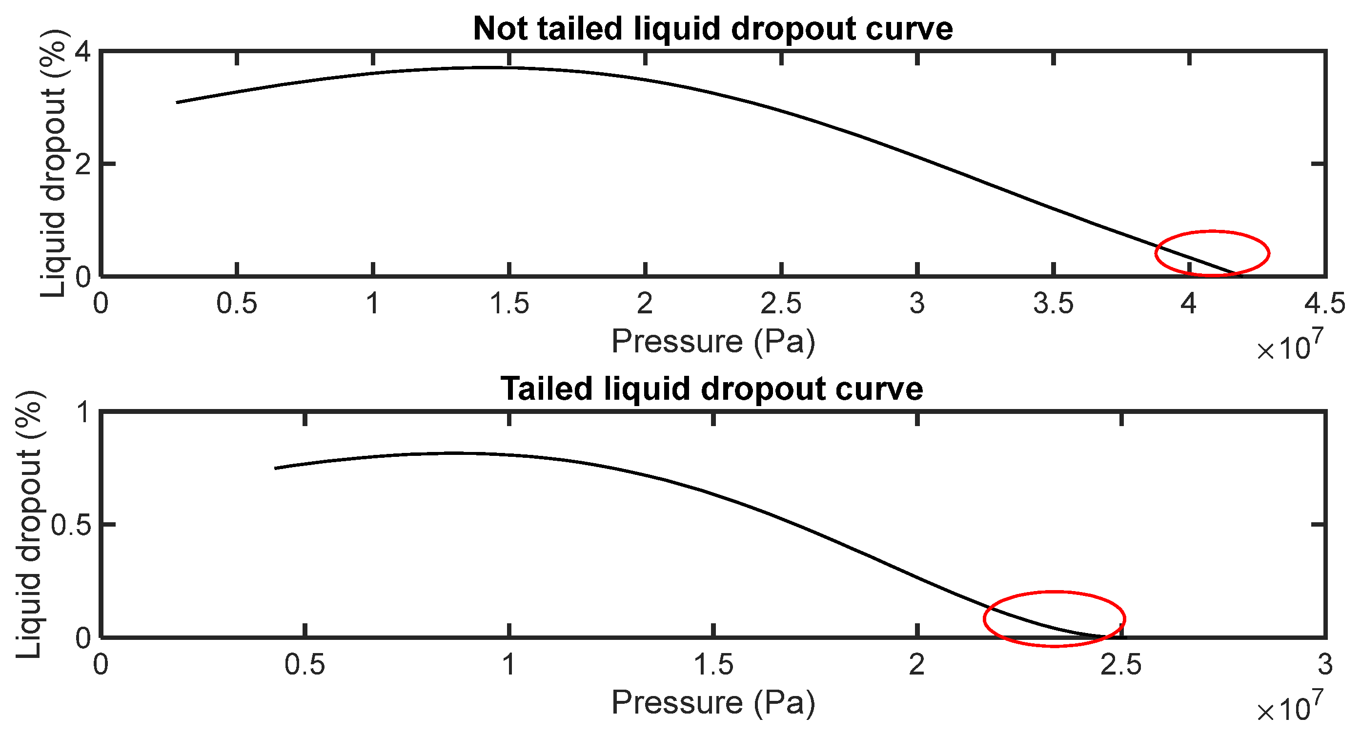
Finally, an experienced fluid expert recognizes that a fine-tuned EoS model must not only accurately reproduce available experimental data but also capture the overall trends specific to the fluid under investigation. For example, the second derivative with respect to pressure (i.e., curvature) of the oil formation volume factor (Bo) curve near the bubble point depends on the oil’s volatility. As a result, for oils with low volatility, the Bo curve in the vicinity of the bubble point takes on a concave downward shape. Conversely, for oils with high volatility, the Bo curve near the bubble point exhibits a concave upward trend, as illustrated in Figure 3. This same principle applies to the solution gas–oil ratio (Rs) curve. In the case of gas condensates, it is worth noting that the shape of the liquid dropout curve varies among different fluids. Some exhibit a distinctive ‘‘tail’’ near the dew point, while others do not, as shown in Figure 4. These observed trends present a unique challenge when trying to capture them using an EoS model. Therefore, operators should carefully apply these constraints during EoS model tuning, drawing upon experimental data obtained from PVT studies.

Figure 3.
Comparison of Bo curve trends near the bubble point for oils with low and high volatility.

Figure 4.
Comparison of liquid dropout curve trends near the dew point.
5. Generalized Pattern Search (GPS) Algorithm
Generalized Pattern Search (GPS) algorithms constitute a subset of direct search methods which aim at locating the global optimum of an error function. Because of their derivative-free nature, GPS algorithms do not require explicit calculation of the gradient of the error function being optimized and can be applied to non-smooth and non-convex optimization problems or problems where gradient information is difficult or even impossible to collect, either because of the CPU time cost or truncation error, as is usually the case for GB algorithms.
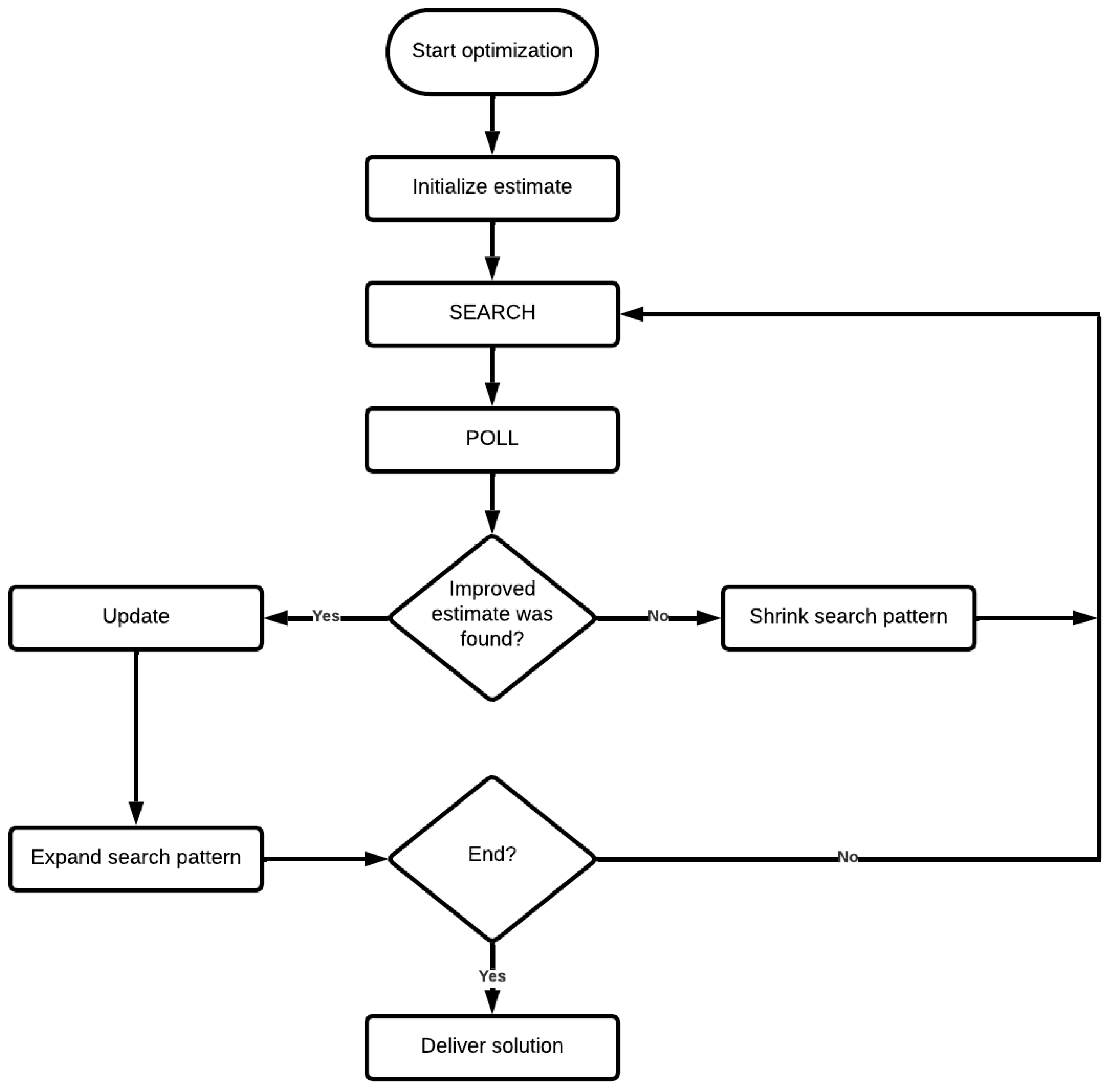
Figure 5 outlines the GPS optimization algorithm logic. The algorithm starts with an initial guess and repeatedly uses two key components: the search step and the poll step. During the search step, the algorithm generates a set of trial points lying around the current best estimate using a group of search directions that define a specific pattern, such as a simplex, box, or cross. The poll step then investigates the performance of the error function at each trial point generated during the search step, replacing the current best estimate with the first trial point that yields a lower value. The search directions are then updated to reflect the new best estimate and the search space is expanded to allow the algorithm to get a ‘‘wider’’ view of the error function shape and avoid getting trapped to a local minimum. The algorithm proceeds with another search step using the updated directions. If the poll step fails to deliver an improved point, the algorithm shrinks the search pattern and explores the region around the current best estimate more closely.
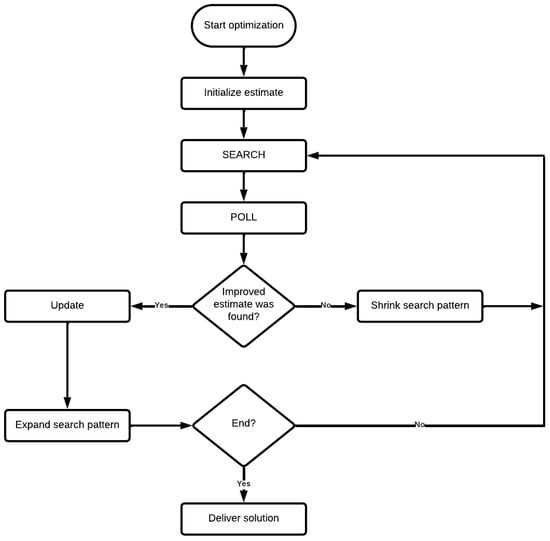
Figure 5.
Outline of the GPS method.
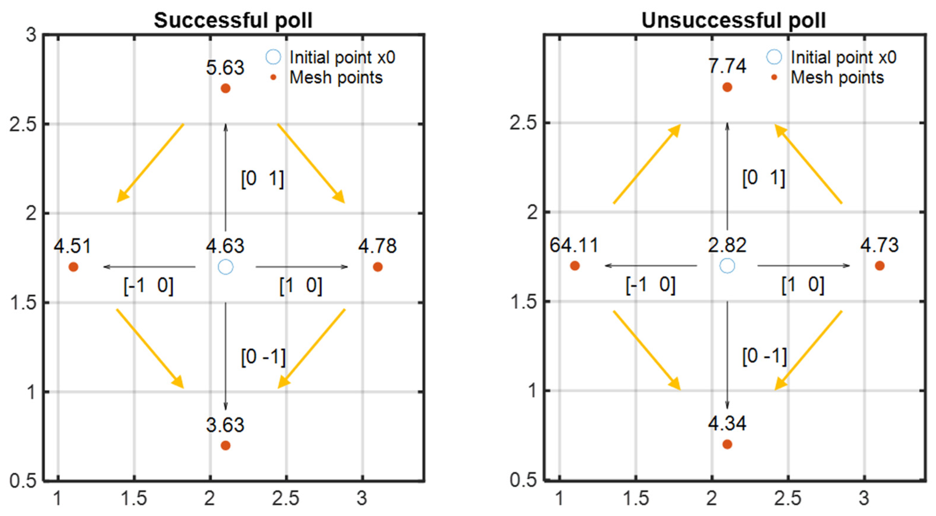
Figure 6 depicts examples of a successful and an unsuccessful poll. In the successful polling scenario, the pattern search begins at current estimate x0 with an initial objective function value of 4.63. In the first iteration, with a mesh size of 1, the GPS algorithm adds the pattern vectors (or direction vectors) [1, 0], [0, 1], [−1, 0], and [0, −1] to x0, generating the mesh points as shown in Figure 5. Subsequently, the GPS algorithm evaluates these mesh points sequentially, in the order previously mentioned, by computing their respective objective function values until it identifies one with a value lower than 4.63. The first such point encountered is x0 + [−1, 0], where the objective value is 4.51. In the case of the unsuccessful polling example, the GPS algorithm is unable to locate a mesh point with an objective value lower than 2.82, corresponding to the objective value of the current estimate x0. The yellow arrows represent the slopes of the objective function surface.
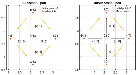
Figure 6.
Illustration of a successful and an unsuccessful poll of the GPS algorithm.
The search and poll steps are repeated until the algorithm converges to an optimal solution or reaches the maximum number of iterations. Moreover, in case of a very high-dimensional error function space, the GPS algorithm makes strategic decisions to omit certain search directions, acknowledging that thoroughly investigating each search direction might pose significant computational challenges.
6. Results and Discussion
6.1. Development of the EoS Tuning Tool
The steps followed to demonstrate the new automated EoS tuning algorithm are described below.
- Development of a PVT simulator
The in-house developed simulator supports both PR [9] and SRK Equations of State (EoS) and can reproduce all standard volumetric PVT experiments conducted in the laboratory, i.e., Constant Composition Expansion (CCE), Constant Volume Depletion (CVD), Differential Liberation Expansion (DLE), and the Lab Separator Test (LST). For stability calculations, Michelsen’s approach [26] is followed to determine whether a phase is thermodynamically stable or unstable for certain pressure and temperature conditions. For single-phase conditions, the molar volume (Vm) is computed using the selected EoS model. For two-phase systems, a flash calculation [27,28] is run utilizing a combination of successive substitutions and the Newton–Raphson method to solve the Rachford–Rice (RR) equation [29]. The saturation pressure is determined using the classic algorithm [12], initialized and safeguarded by a bisection method. These codes can be combined to emulate any routine PVT study and eventually evaluate objective function J at any iteration of the GPS algorithm.
- 2.
- Grouping of the input data
Input data is organized into three major categories and stored in structures. The first category includes the initialized EoS model parameters and reservoir conditions. PVT laboratory measurements and experimental specifications (such as the pressure at each CCE or DLE step) fall into the second category, whereas the third category contains the weighting factors of the fluid properties at each pressure step to be utilized in the calculation of the error function. The weighting factors need to be determined based on the discussion in Section 3, which involves considering the relative importance of each variable and assigning appropriate weights accordingly.
- 3.
- Implementation of the GPS algorithm
To serve the objectives of this study, a dedicated MATLAB function was developed to evaluate the error function to be minimized, considering the experimental data from each available PVT study conducted on the investigated fluid, along with the EoS predictions and further combined to the weights selected. This function holds significant importance in fine-tuning the EoS, as it provides engineers with a concrete means to evaluate the accuracy of their predictive models.
The automated tuning approach utilized the GPS method which is implemented in MATLAB’s Global Optimization Toolbox. It should be mentioned that, although coding the GPS algorithm is generally considered straightforward, with many open-source implementations available in repositories, the choice to utilize the functionality within MATLAB’s toolbox was made for smoother integration into the existing PVT research framework. All physical constraints discussed in Section 4 were coded and introduced as box, linear, or nonlinear equality or inequality constraints into the EoS tuning tool. Finally, it is important to note that, in this work, the GPS method was employed with the default options provided by MATLAB [30] for parameters such as the maximum number of iterations or search directions allowed.
6.2. Examples
In this work, the PR EoS [9] was utilized for its wide application in the industry and its improved accuracy in calculating liquid density. A gas condensate and an H2S-rich oil were used to investigate the efficiency of the proposed optimization method in minimizing the objective function in Equation (1). Prior to implementing the global optimization method in real reservoir fluids, a thorough check to ensure the consistency and validity of the available lab PVT data was carried out. Note that the experimental data on the gas condensate and the H2S-rich fluid used in this work were generated through in-house experimental measurements on received reservoir fluid samples. By performing a quality control (QC) analysis on the experimental data, potential errors, discrepancies, or inaccuracies within the dataset can be identified and rectified, if needed. This verification process ensures that the data used for implementing the automated tuning methodology accurately represents the actual characteristics and behavior of the reservoir fluids being studied.
The accuracy of the tuned EoS models was assessed using the Absolute Average Relative Deviation (AARD) formula:
where and are the experimental and model estimated PVT values, respectively, while stands for the number of experimental points considered.
For the gas condensate optimization problem, in addition to the GPS algorithm, a conventional gradient-based (GB) constrained optimizer was used to examine the superiority of the former over the latter. To reduce the possibility of getting stuck to a local minimum, the GB optimizer was run 100 times using different random starting points, unlike the GPS optimizer which was run only once. This approach was adopted because the GB algorithm is a local optimization method and, as such, it will only track down local minima.
6.3. Results
6.3.1. Gas Condensate
The first fluid used to assess the performance of the GPS algorithm is a gas condensate mixture. Table 1 provides information on the components of the gas condensate after characterizing the C7+ fraction of this fluid and applying some minor pseudoization to the EoS model. F1, F2, F3, and F4 denote the heavy lumped pseudos that represent the composition of the C7+ fraction within the mixture. Further component lumping, according to the workflow described in Section 2, may have been possible but was not attempted as the exact process which would be simulated with the tuned EoS model was not known in advance.

Table 1.
Composition of gas condensate after C7+ characterization.
Two different tuning approaches were tried to optimize the performance of the EoS for modeling the gas condensate fluid behavior. This way, the globality of the GPS method can be demonstrated, given that both tuning approaches used the GPS method with the same starting point. The first approach only adjusted the properties of the MCN components with the highest concentration in the mixture (pseudos F1 and F2), while the second approach extended its scope to include all four MCN components. In both tuning approaches, the adjustable parameters included the critical properties Pc and Tc, the acentric factors, and the volume shift parameters of the selected heavy lumped pseudo-components. Additionally, the binary interaction coefficients (BICs) between each selected pseudo-component and N2C1 were selected for adjustment, due to the notably high concentration of N2C1 within the mixture.
As previously stated, the initial approach to address the EoS tuning problem involved adjusting the properties of pseudos F1 and F2 only, given their considerably higher concentrations compared to all other MCN components in the gas condensate mixture. Nevertheless, moderate only results are expected when such a limited tuning parameters set is iterated as condensate properties do depend on all four pseudos.
Table 2 and Table 3 and Figure 7 provide a comparison of the estimations derived from the PR EoS, tuned using the GPS and the GB methods, against the experimental saturation pressure and CVD data. For the GB method, only 20 out of 100 trials led to acceptable EoS tuning results whereas the other ones got trapped in a poor local minimum. A solution obtained from a poor starting point is intentionally showcased in Table 2 and Table 3 and Figure 7. This choice serves to underscore the need to employ the GB method with various initial points since the algorithm is prone to getting trapped to a local minimum. Indeed, the initial guess led to poor predictions for the saturation pressure with an AARD% of 15.46%, which further results in poor CVD property estimations. Such poor-quality results were obtained for 80% of the various GB runs, demonstrating how labor-intensive it is to achieve adequate results with the GB method.
Table 2.
Experimental and estimated dew point pressure—Approach 1.
Table 3.
AARD% values—Approach 1.
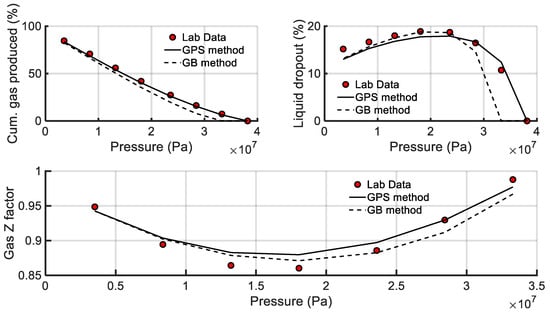
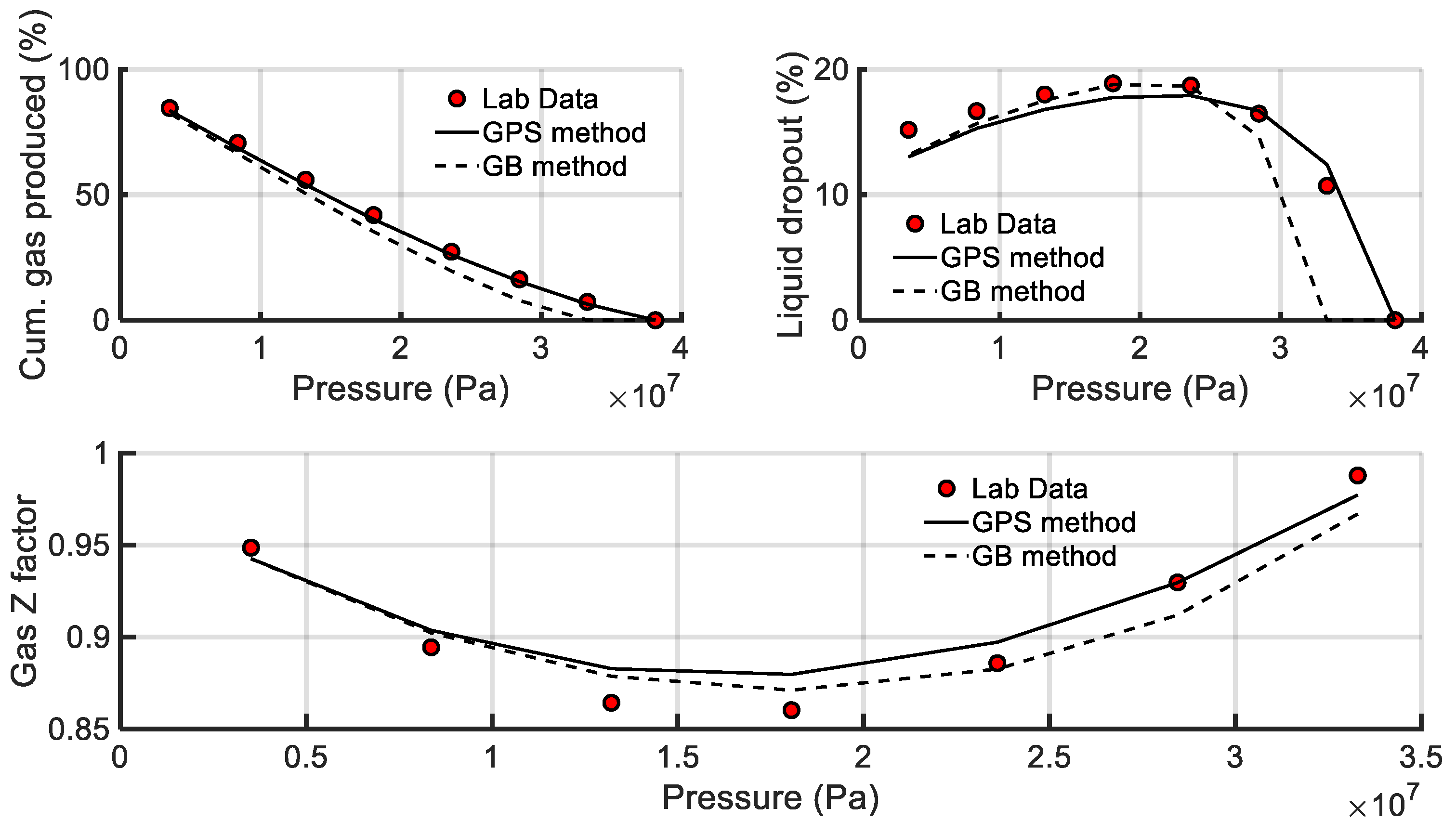
Figure 7.
Estimates of the volumetric property predictions against CVD experimental data—Approach 1.
On the contrary, the GPS method, as a global optimization approach, did not require multiple starting points to converge to an adequate solution. As seen in Table 2 and Table 3, the GPS algorithm provides fine predictions for key PVT values, including dew point pressure, cumulative gas produced, liquid yield, and gas compressibility factor (gas Z factor), which exhibit AARDs lower than 3%, 5%, 8%, and 2%, respectively.
In the second tuning approach, adjustments were made to the properties of all four MCN components, making this approach more comprehensive compared to the first one. Similarly to the first approach, both GPS and GB algorithms were used to fine-tune the PR EoS. Results in Table 4 and Table 5 and Figure 8 show GB’s incompetence at precisely reproducing the available laboratory data when the initial guess is poor. It is interesting to note that, out of the 100 different solutions obtained by selecting random starting parameter vectors, only 3 acceptable solutions were derived, indicating that, as the dimensionality of the optimization problem becomes higher, the efficiency of the GB algorithm decreases.
Table 4.
Experimental and estimated dew point pressure—Approach 2.
Table 5.
AARD% values—Approach 2.
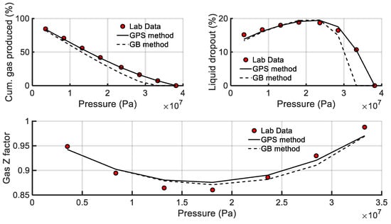
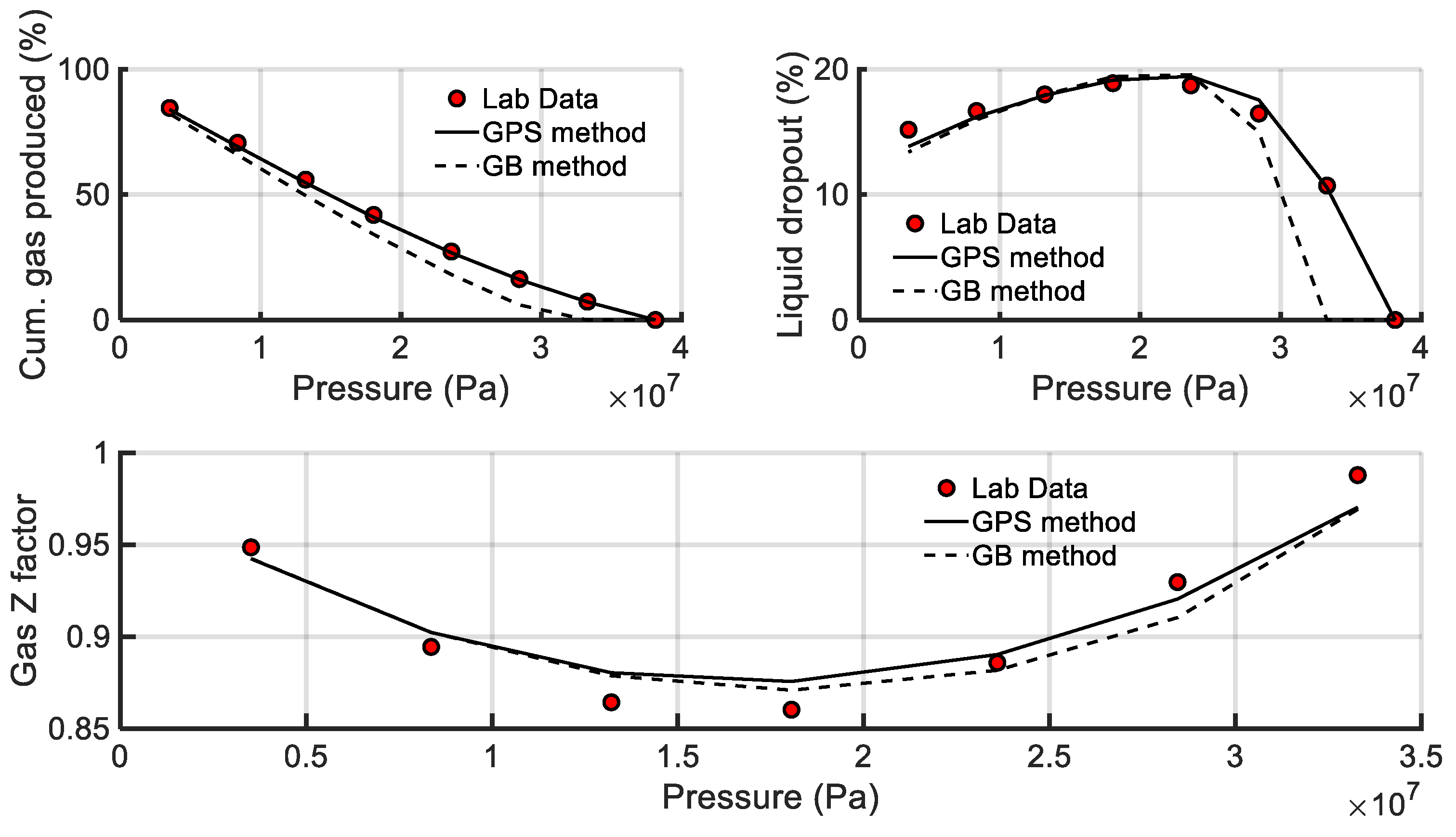
Figure 8.
Estimates of the volumetric property predictions against CVD experimental data—Approach 2.
As anticipated, the accuracy of the GPS-tuned model improved (Table 4 and Table 5) with an increase in the number of tunable parameters, which confirms the globality of the method. Table 5 shows that the GPS-tuned model now exhibits AARDs less than 1%, 2%, 4%, and 2% for the dew point pressure, cumulative gas produced, liquid yield, and gas Z factor, respectively. This is a significant improvement over the results obtained with the GPS algorithm in the first tuning approach.
In both tuning approaches, the unconstrained GB and GPS optimizer consistently violated the hierarchy of Pc and Tc of the heavy lumped pseudos as well as the kijs’ allowed range (i.e., box constraint). To preserve those fundamental principles, the constraints specified in Equations (2) and (3) were imposed on the GPS algorithm, which successfully recovered the correct order of the component properties in the tuned EoS model. It is worth noting that the constraint in Equation (4) was intentionally skipped because the volume shift parameters of the heavy lumped pseudos were tuned rather than their molecular weights.
6.3.2. H2S-Rich Oil
Subsequently, the GPS optimizer was tested on a reservoir oil with a H2S concentration of 31.43%. Note that this composition represents the reservoir fluid of an oil field in Northern Greece [31,32], the high H2S content of which poses a significant challenge in EoS model tuning due to the polar nature of H2S. The developed EoS model will be utilized for simulating an Enhanced Oil Recovery (EOR) process that includes acid gas (primarily comprising H2S and CO2) injection. According to the workflow outlined in Section 2, the heavy end was split into single carbon number (SCN) fractions which were further lumped into three pseudo-components to maintain the number of components as low as possible. The final composition comprises 11 components, wherein N2 and C1 are grouped together as N2C1, while C4 and C5 isomers are combined into two components. Given the significant concentration of H2S in the oil sample, and the fact that the developed EoS model will be utilized to account for the acid gas phase behavior, H2S was maintained as a distinct component. The composition of the lumped model is given in Table 6.
Table 6.
Composition of the H2S-rich oil.
The reported PVT values indicate that this reservoir fluid’s phase behavior is quite intriguing. In the undersaturated area, compressibility decays unexpectedly fast, although the light components account for more than 50% of the total composition. Additionally, the liberated gas specific gravity is unusually high due to the presence of high H2S content. The parameters selected for tuning were the critical properties (Pc, Tc), acentric factors, and volume shift parameters of the three heavy pseudos, as well as the BICs of each one of them with C1 and H2S. Higher weight values were set to the PVT properties values close to the bubble point as those prevailing to very low pressure are not prone to be utilized during a reservoir or wellbore flow simulation.
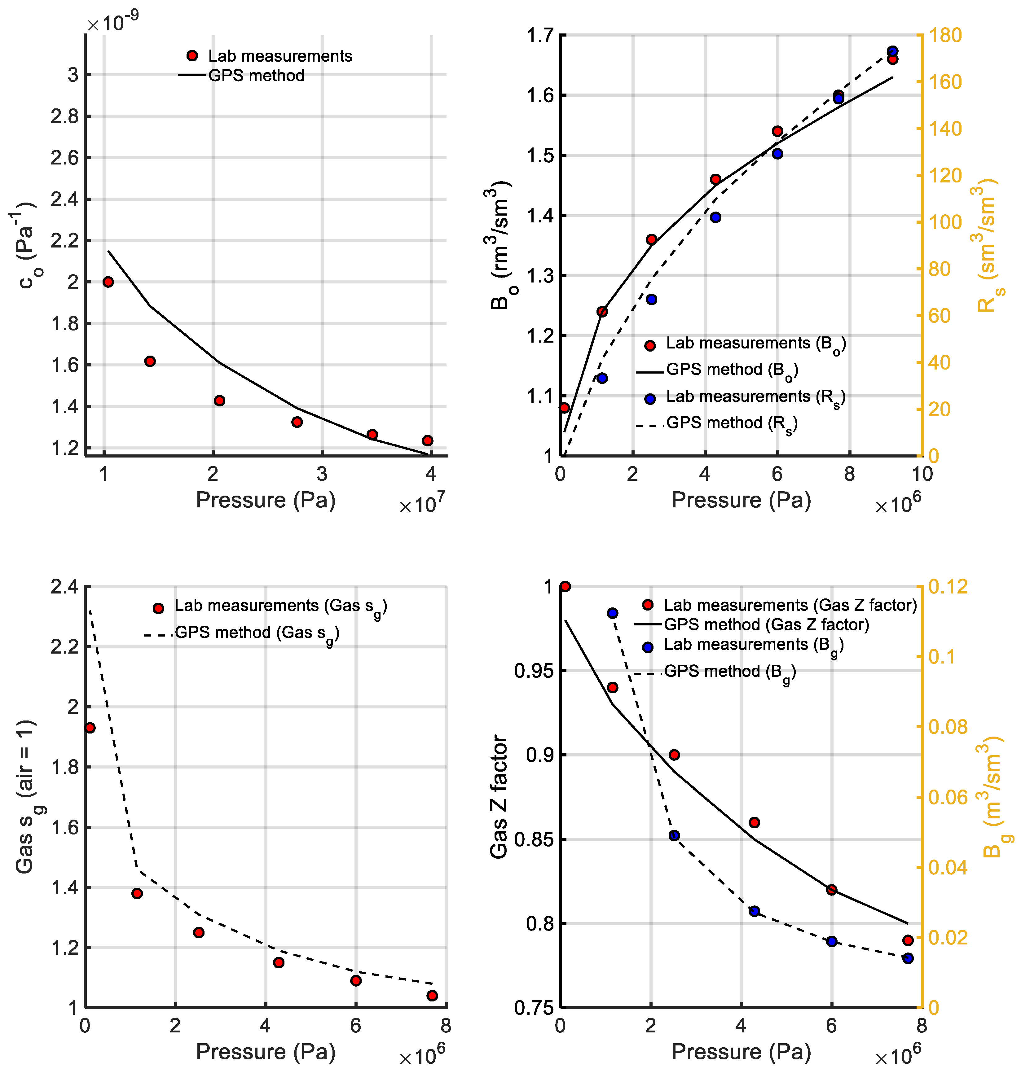
The results of the sole run of the GPS tuning of the EoS against the measured data obtained for the saturation pressure, CCE, DLE, and LST data at 118 °C are shown in Table 7, Table 8 and Table 9 and Figure 9. Despite its peculiarity, isothermal compressibility (co) in the single-phase region of the fluid was matched with an AARD% of approximately 6%. Note that this deviation corresponds to an AARD of less than 0.5% for the single-phase oil formation volume factor (Bo) and density values due to fact that compressibility is integrated to provide the relative volume. Bo and dissolved-gas-to-oil ratio (Rs) proved to be accurately reproduced over the high-pressure range of the two-phase region; the same is true for the gas formation volume factor (Bg), gas compressibility factor (gas Z factor), and gas specific gravity (sg), with AARD% values of less than 4%. Finally, the available LST data were excellently reproduced by the GPS-tuned model.
Table 7.
Experimental and estimated bubble point pressure.
Table 8.
Experimental and estimated LST data.
Table 9.
AARD% values.
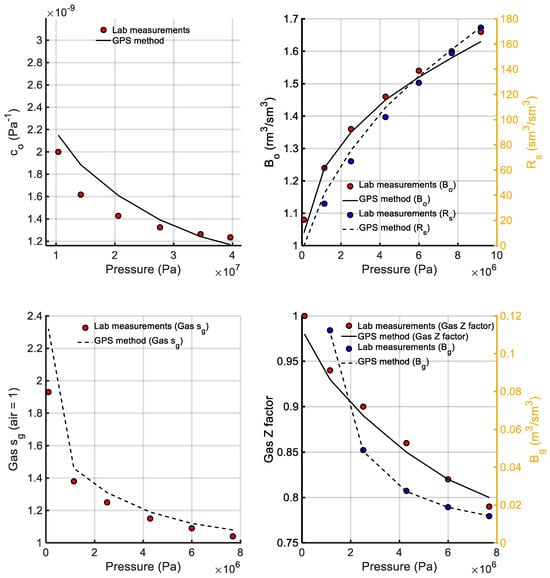
Figure 9.
Estimates of the volumetric property predictions against CCE and DLE experimental data.
7. Conclusions
This study addresses the challenge of accurately tuning Equations of State (EoS) models to describe the thermodynamics of hydrocarbon systems under varying conditions. Recognizing that accurate EoS models are of significant importance for running successful reservoir and pipeline simulations within the oil and gas industry, this paper outlines the standard workflows followed by reservoir engineers to tune an EoS model. It introduces a new approach to EoS tuning through the utilization of a Generalized Pattern Search (GPS) algorithm. This algorithm has been selected due to its capability of navigating intricate high-dimensional search spaces effectively, avoiding local optima and thereby enhancing the probability of arriving at globally optimal solutions. This feature is especially significant when dealing with the inherent complexity and high nonlinearity of EoS tuning as conventional local (gradient-based, mostly) optimization methods are prone to get stuck in a poor solution (local minimum) which most probably will not represent the real potential of the EoS model. Furthermore, the developed EoS tuning tool accommodates not only box constraints, as commonly observed in EoS tuning research, but also the integration of various complex physical constraints which the tuned EoS model needs to satisfy to ensure sound predictions. This dual consideration ensures that the tuned EoS models not only align with experimental data but also adhere faithfully to fundamental thermodynamic principles.
This work contributes significantly to the domain of reservoir engineering by offering an automated solution to a long-standing obstacle. The ability to attain accurate EoS tuning with minimal dependence on operator experience is a notable advancement, minimizing subjectivity and enhancing the efficiency of the tuning process. Consequently, this methodology holds the potential to drive enhancements in reservoir and pipeline simulations, ultimately leading to more informed decision-making within the oil and gas sector.
Author Contributions
Conceptualization, E.M.K. and V.G.; methodology, E.M.K.; software, E.M.K.; validation, E.M.K. and V.G.; writing—review and editing, E.M.K. and V.G.; visualization, E.M.K.; supervision, V.G. All authors have read and agreed to the published version of the manuscript.
Funding
This research received no external funding.
Data Availability Statement
Data are contained within the article.
Conflicts of Interest
The authors declare no conflicts of interest.
References
- Gaganis, V.; Anastasiadou, V. A generalized flash algorithm to bridge stability analysis and phase split calculations. Fluid Phase Equilibria 2023, 565, 113625. [Google Scholar] [CrossRef]
- Whitson, C.H.; Martinsen, S.Ø.; Younus, B. Sampling Petroleum Fluids; Elsevier: Amsterdam, The Netherlands, 2022; pp. 41–93. [Google Scholar]
- Ahmed, T. Equations of State and PVT Analysis; Elsevier: Amsterdam, The Netherlands, 2013. [Google Scholar]
- Kathrada, M.; Fuenmayor, A. Characterisation of Hydrocarbon Fluids for Integrated Production Modelling. In Proceedings of the SPE Middle East Oil and Gas Show and Conference, Manama, Bahrain, 10–13 March 2013. [Google Scholar]
- Chen, Z. Reservoir Simulation: Mathematical Techniques in Oil Recovery; Society for Industrial and Applied Mathematics: University City, PH, USA, 2007. [Google Scholar]
- Fevang, Ø.; Singh, K.; Whitson, C.H. Guidelines for choosing compositional and black-oil models for volatile oil and gas-condensate reservoirs. In Proceedings of the SPE Annual Technical Conference and Exhibition, Dallas, TX, USA, 1–4 October 2000. [Google Scholar]
- Voskov, D.V.; Tchelepi, H.A. Comparison of nonlinear formulations for two-phase multi-component EoS based simulation. J. Pet. Sci. Eng. 2012, 82–83, 101–111. [Google Scholar] [CrossRef]
- Peng, D.Y.; Robinson, D.B. A new two-constant equation of state. Ind. Eng. Chem. Fundam. 1976, 15, 59–64. [Google Scholar] [CrossRef]
- Robinson, D.B.; Peng, D.Y. The Characterization of the Heptanes and Heavier Fractions; Gas Processors Association: Tulsa, OK, USA, 1978. [Google Scholar]
- Soave, G. Equilibrium constants from a modified Redlich-Kwong equation of state. Chem. Eng. Sci. 1972, 27, 1197–1203. [Google Scholar] [CrossRef]
- Wilhelmsen, Ø.; Aasen, A.; Skaugen, G.; Aursand, P.; Austegard, A.; Aursand, E.; Gjennestad, M.A.; Lund, H.; Linga, G.; Hammer, M. Thermodynamic Modeling with Equations of State: Present Challenges with Established Methods. Ind. Eng. Chem. Res. 2017, 56, 3503–3515. [Google Scholar] [CrossRef]
- Whitson, C.H.; Brulé, M.R. Phase Behavior; SPE Monograph Series; Society of Petroleum Engineers Inc.: Richardson, TX, USA, 2000. [Google Scholar]
- Zahedizadeh, P.; Osfouri, S.; Azin, R. Accurate, Cost-Effective Strategy for Lean Gas Condensate Sampling, Characterization, and Phase Equilibria Study. J. Pet. Sci. Eng. 2022, 210, 110085. [Google Scholar] [CrossRef]
- Ali, M.; El-Banbi, A. EOS Tuning—Comparison between Several Valid Approaches and New Recommendations. In Proceedings of the SPE North Africa Technical Conference and Exhibition, Cairo, Egypt, 14–16 September 2015; OnePetro: Dubai, United Arab Emirates, 2015. [Google Scholar]
- Sarvestani, M.T.; Sola, B.S.; Rashidi, F. Genetic Algorithm Application for Matching Ordinary Black Oil PVT Data. Pet. Sci. 2012, 9, 199–211. [Google Scholar] [CrossRef]
- Zarifi, A.; Daryasafar, A. Auto-Tune of PVT Data Using an Efficient Engineering Method: Application of Sensitivity and Optimization Analyses. Fluid Phase Equilibria 2018, 473, 70–79. [Google Scholar] [CrossRef]
- Coats, K.H.; Smart, G.T. Application of a Regression-Based EOS PVT Program to Laboratory Data. SPE Reserv. Eng. 1986, 1, 277–299. [Google Scholar] [CrossRef]
- Christensen, P.L. Regression to Experimental PVT Data. J. Can. Pet. Technol. 1999, 38, PETSOC-99-13-52. [Google Scholar] [CrossRef]
- Aguilar Zurita, R.A.; McCain, W.D. An efficient tuning strategy to calibrate cubic EOS for compositional simulation. In Proceedings of the SPE Annual Technical Conference and Exhibition, San Antonio, TX, USA, 29 September–2 October 2000. [Google Scholar]
- Pedersen, K.; Thomassen, P.; Fredenslund, A. Phase Equilibria and Separation Processes; Report SEP 8207; Institute for Kemiteknik, Denmark Tekniske Hojskole: Copenhagen, Denmark, 1982. [Google Scholar]
- Whitson, C.H. Characterizing hydrocarbon plus fractions. SPE J. 1983, 23, 683–694. [Google Scholar] [CrossRef]
- Coats, K.H. Simulation of gas condensate reservoir performance. J. Pet. Technol. 1985, 37, 1870–1886. [Google Scholar] [CrossRef]
- Chueh, P.L.; Prausnitz, J.M. Vapor-liquid equilibria at high pressures: Calculation of partial molar volumes in nonpolar liquid mixtures. AIChE J. 1967, 13, 1099–1107. [Google Scholar] [CrossRef]
- Computer Modelling Group (CMG) Ltd. WinProp Fluid Property Characterization Tool. Available online: https://www.cmgl.ca/winprop (accessed on 15 September 2023).
- Gaganis, V.; Varotsis, N.; Nighswander, J.; Birkett, G. Monitoring PVT Properties Derivatives Ensures Physically Sound Tuned EOS Behaviour Over the Entire Operating Conditions Range. In Proceedings of the 67th EAGE Conference & Exhibition, Madrid, Spain, 13–16 June 2005; European Association of Geoscientists & Engineers: Utrecht, The Netherlands, 2005. [Google Scholar]
- Michelsen, M.L. The isothermal flash problem. Part I. Stability. Fluid Phase Equilibria 1982, 9, 1–19. [Google Scholar] [CrossRef]
- Michelsen, M.L. The isothermal flash problem. Part II. Phase-split calculation. Fluid Phase Equilibria 1982, 9, 21–40. [Google Scholar] [CrossRef]
- Kanakaki, E.M.; Samnioti, A.; Gaganis, V. Enhancement of Machine-Learning-Based Flash Calculations near Criticality Using a Resampling Approach. Computation 2024, 12, 10. [Google Scholar] [CrossRef]
- Rachford, H.H., Jr.; Rice, J.D. Procedure for use of electronic digital computers in calculating flash vaporization hydrocarbon equilibrium. J. Pet. Technol. 1952, 4, 19. [Google Scholar] [CrossRef]
- The MathWorks Inc. Optimization Toolbox for Use with MATLAB R®. User’s Guide for Mathworks; The MathWorks Inc.: Natick, MA, USA, 2022. [Google Scholar]
- Samnioti, A.; Kanakaki, E.M.; Koffa, E.; Dimitrellou, I.; Tomos, C.; Kiomourtzi, P.; Gaganis, V.; Stamataki, S. Wellbore and reservoir thermodynamic appraisal in acid gas injection for EOR operations. Energies 2023, 16, 2392. [Google Scholar] [CrossRef]
- Kanakaki, E.M.; Samnioti, A.; Koffa, E.; Dimitrellou, I.; Obetzanov, I.; Tsiantis, Y.; Kiomourtzi, P.; Gaganis, V.; Stamataki, S. Prospects of an Acid Gas Re-Injection Process into a Mature Reservoir. Energies 2023, 16, 7989. [Google Scholar] [CrossRef]
Disclaimer/Publisher’s Note: The statements, opinions and data contained in all publications are solely those of the individual author(s) and contributor(s) and not of MDPI and/or the editor(s). MDPI and/or the editor(s) disclaim responsibility for any injury to people or property resulting from any ideas, methods, instructions or products referred to in the content. |
© 2024 by the authors. Licensee MDPI, Basel, Switzerland. This article is an open access article distributed under the terms and conditions of the Creative Commons Attribution (CC BY) license (https://creativecommons.org/licenses/by/4.0/).