Thermodynamic Modeling of Mineral Scaling in High-Temperature and High-Pressure Aqueous Environments

Abstract

Methods of predicting mineral scale formation have evolved over the years from simple empirical fittings to sophisticated computational programs. Though best practices can now solve complex multi-phase, multi-component systems, they are largely restricted to temperatures below 300 °C. This review examines critical gaps in existing mineral scale modeling approaches as well as strategies to overcome them. Above 300 °C, the most widely used model of standard thermodynamic functions for aqueous species fails when fluid densities are below 0.7 g cm⁻³. This failure occurs due to the model’s reliance on an empirical form of the Born equation which is unable to capture the trends observed in these high temperature, low density regimes. However, new models based on molecular solvent-solute interactions offer a pathway to overcome some of the deficiencies currently limiting high-temperature and high-pressure mineral scale predictions. Examples of the most common scale prediction methods are presented, and their advantages and disadvantages are discussed.

1. Introduction

The safety and reliance of many engineering applications rely on the prediction of operating scenarios that lead to severe mineral scale formation events. A classic example of the immediate and dramatic effects of scale formation is an event that occurred during early production from the Miller oil field which brought production of 30,000 barrels a day to zero in 24 h [1]. Knowledge of scaling conditions inform operating decisions that directly affect lifetime and safety [2]. As such, methods of modeling mineral solubility, which is the driving force for scale formation, date back to the early 1900s and are still being improved today. When available, mineral scale models can be used to (i) avoid mixing of incompatible brines, (ii) determine if scale inhibitors are needed and (iii) predict when scale removal maintenance is required [2,3]. Some common mineral scales are sulfate-based (Ba, Sr, Ca), oxides/hydroxide-based (Fe, Mg), and carbonate-based (Ca, Mg, Fe) [2]. However, the development of models to predict the formation of all these possibilities is an ongoing effort with many challenges due to the number of possible conditions that lead to mineral scale formation.

Determining the thermodynamic favorability of mineral scale formation is the first and most important step in combating mineral scaling. Thermodynamic favorability is governed by a mineral’s solubility limit (b_sat) and whether a particular fluid is above or below that limit. As such, knowing b_sat is paramount to effective mineral scale control. To better predict b_sat, the modeling of how it changes with system conditions has evolved from simple polynomials [4,5] to sophisticated thermodynamic programs [6,7,8,9] containing computational algorithms and thermodynamic databases [10,11,12]. This progression was a necessary response to the increasing complexity and diversity of how different mineral solubility limits change with the composition, temperature and pressure of fluids observed in applications which now range from low-temperature, low-pressure (LTLP) to high-temperature, high-pressure (HTHP) conditions [2,3]. Though complex, it is vital that thermodynamic models reliably capture these trends because system properties (temperature, pressure, etc.) vary dramatically within a system which can promote scaling in different regions (see Figure 1).

The solubility limits of a mineral depend strongly on the capacity of a solution to solubilize the solute species needed to form that mineral. This capacity is called the ion activity product (IAP), and it is used with a solubility product (K_sp) to assess a fluids tendency for scale formation [14,15]. This tendency is quantified with what is known as the scale saturation ratio (SR),

$$SR=\frac{IAP}{K_{\mathrm{sp}}}$$

(1)

which is a ratio of the IAP to K_sp for a given mineral [14,15].

For barite, a common scale in oil and gas applications, the SR is determined as follows:

$$SR\left(\mathrm{Barite}\right)=\frac{a_{{\mathrm{Ba}}^{2+}\left(\mathrm{aq}\right)}{a}_{{\mathrm{SO}}_4{}^{2-}\left(\mathrm{aq}\right)}}{K_{\mathrm{sp},{ \mathrm{BaSO}}_4\left(\mathrm{s}\right)}}$$

(2)

where $a_{{\mathrm{Ba}}^{2+}\left(\mathrm{aq}\right)}$ is the activity of barium ions and $a_{{\mathrm{SO}}_4{}^{2-}\left(\mathrm{aq}\right)}$ is the activity of sulfate ions within the solution. The IAP value represents the activities of species present in the solution, which can deviate from what is thermodynamically stable, and is affected by side reactions with other chemical species also within the solution [14]. Setting aside the non-thermodynamic contributions (e.g., kinetics of scaling), the influence of possible side reactions with additional chemical species is no trivial matter and a primary driver of the steady evolution of models to predict the solubility limit of minerals that account for multi-phase, multi-component contributions.

Many publications address the modeling of mineral solubility limits; all of which can be sub-divided into three distinct strategies that have certain advantages and disadvantages. However, the option to use a particular method depends strongly on the availability of specific datasets. Over the last 40 years, the three options most frequently used are (i) empirical data fits of experimental data from solubility experiments, (ii) thermodynamic calculation of solubility products from thermodynamic databases, and (iii) multi-phase, multi-component computational thermodynamic programs. The first approach requires experimental solubility limit data for the system of interest, whereas the last two approaches leverage databases and publications that provide standard partial molar Gibbs energy values for the species of interest to these models. Each method can be further sub-divided to differentiate the range of sub-techniques used to obtain solubility limits of scaling minerals (see Figure 2).

Though empirical fits are often the easiest to apply and the most readily available for simple systems, they have been steadily phased out from use for multi-phase, multi-component environments.

Because a number of reviews have already been conducted on mineral scale modeling strategies, we will briefly draw attention to some of their main findings to emphasize how this review differs. A few recent publications have identified important deficiencies in scale modeling methods for the petroleum and natural gas industry up to 200 °C. They found that the availability of experimental data [16,17] and shortcomings in activity coefficient modeling databases are both impeding reliable mineral scale modeling efforts [16,18]. A few studies have also stressed the need to incorporate multi-phase, multicomponent features into scale modeling practices given their significant impact to several important mineral scale chemistries [16,18]. Other studies have focused on the role of scale mitigation strategies through the use of inhibitors [17,19,20]. However, none of these works discuss the underlying model limitations for the standard thermodynamic functions that underpin many of these modeling methods if extended to temperatures above 300 °C. Likewise, the internal consistency and viability of available standard Gibbs energy and equilibrium constant data used by many scale modeling programs are rarely discussed. Here, we provide a general overview of basic scale modeling methods, discuss overlooked technical gaps still present in commonly used standard thermodynamic functions and highlight strategies to overcome them.

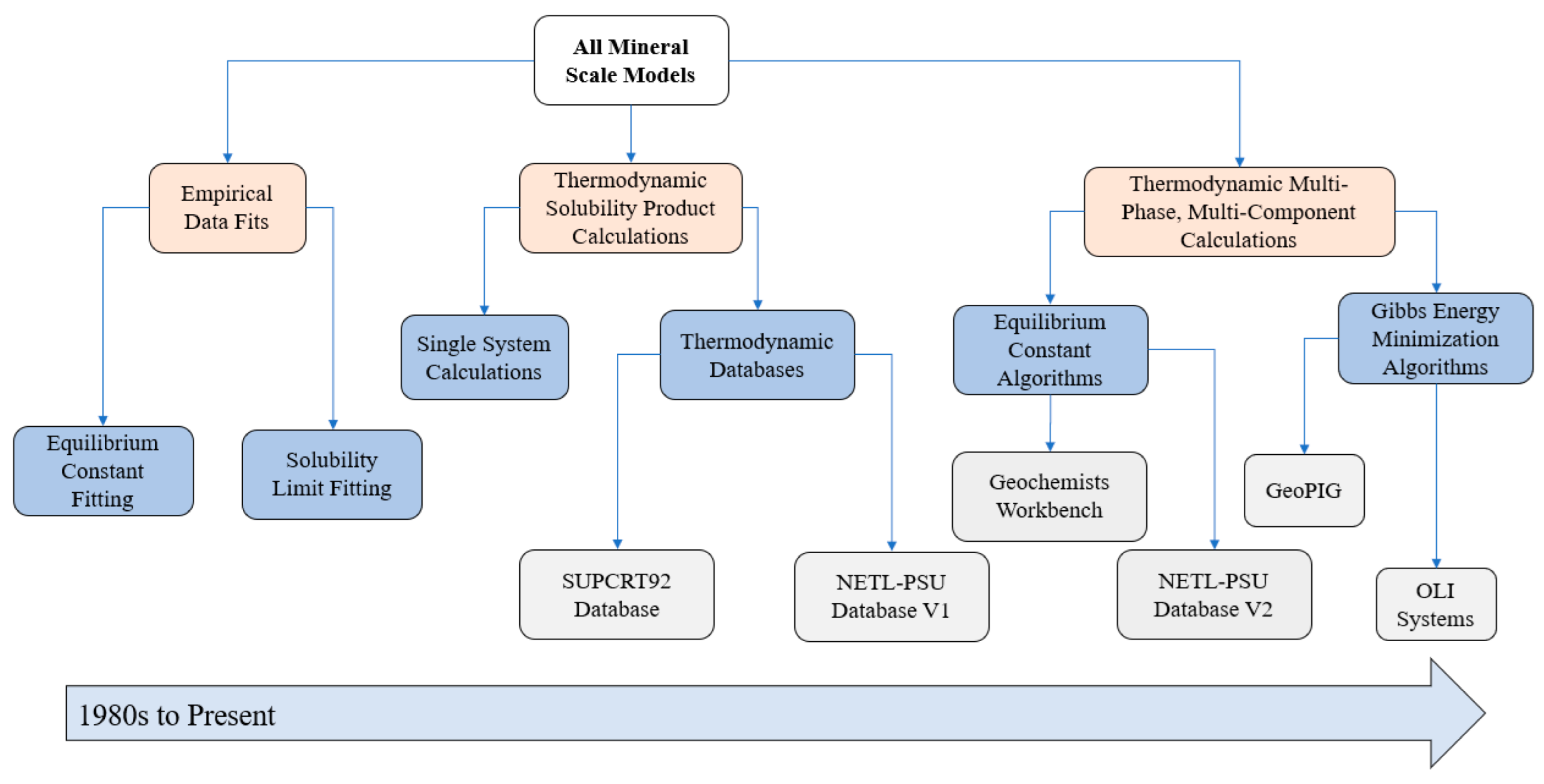
2. Empirical Fitting Methods

One of the earliest methods for modeling the solubility limits of mineral scale were basic empirical fits of solubility data. Prior to the early 1980s, the partial molar standard Gibbs energy data required to determine the thermodynamic driving force for mineral scale deposition reactions were not readily accessible or known for many conditions [21]. A good example of this method is calcium carbonate mineral scale in pure water and saltwater environments [5,22]. These empirical fits were used to model solubility limits for specific systems with known compositions, temperatures, and pressures. As such, they were frequently updated as more experimental data became available; in many instances, this approach remains the best way to compile data from multiple experimental studies.

Most empirical solubility models are basic polynomials with the minimum number of parameters needed to get a satisfactory fit (i.e., a high R² value). These models either fit an equilibrium constant for a mineral precipitation reaction (solubility product) or a solubility limit concentration itself [4,5,22,23,24]. The choice of solubility product over solubility limit was often based on the desired use of the final fitting. Earlier works often focused on obtaining the solubility products, since these were not known for many mineral reactions, whereas later works focused on the solubility limits since these values are often used to validate new thermodynamic models for predicting mineral precipitation conditions.

A notable example of the simple empirical method for solubility limits was demonstrated by Krumgalz [4,23,24]. His three-part publication series analyzed over a thousand publications with mineral solubility data to formulate empirical fits of the solubility limits for alkaline and alkaline earth sulfates, chlorides and bromides at elevated temperatures. The cations examined in each publication were sodium, potassium, magnesium, calcium, strontium and barium, and the anions were chlorides, bromides, and sulfates. The temperature range varied from mineral to mineral because they were limited by the availability of experimental data. Generally, several of the minerals were fit for a range of 0 to 300 °C. The systems analyzed were the mineral of interest in pure water for a series of different temperatures. Each of these minerals were fit to a polynomial that had up to six of the following terms:

b_sat = a₀ + a₁t + a₂t² + a₃t³ + a₄t⁴ + a₅t⁵ + a₆t⁶

(3)

where t is the temperature is Celsius, and a₀–a₆ are empirical constants used to fit the experimental data. As such, this empirical model provides reliable mineral solubility limits for the water-mineral system over a given temperature range. The work by Krumgalz demonstrates both the impact of temperature on the solubility of common minerals, and how they can vary dramatically between minerals for the same set of conditions (see Figure 3).

Of the minerals analyzed, most fits obtained had an R² of 0.98 or better, with only three of the six empirical constants, but the number of constants required typically increased with the temperature range. Three to six terms are required for simple systems over small temperature ranges, it becomes increasingly difficult to accommodate additional dependences such as composition and pressure changes without a model being inundated by empirical constants.

Though less common now, this empirical approach has been used to capture the impact of more than one independent variable. Examples can be found as far back as the early 1980s, when scientists were documenting the solubility product (K_sp) of calcium carbonate minerals in different seawater salinities for a range of temperatures [5,22]. Their goal was to model both the temperature and salinity dependences of calcium carbonate. The resulting model to capture temperature and salinity trends are as follows:

log₁₀K_sp = a₀ + a₁T + a₂T⁻¹ + a₃log₁₀(T) + (b₀ + b₁T + b₂T⁻¹)S^0.5 + c₀S + d₀S^1.5

(4)

where a₀–a₃, b₀–b₂, c₀ and d₀ are all the empirical constants needed to model the dependence of the solubility product on salinity (S), (from 5 to 44 ppt), and temperature (T), (from 278.15 to 313.15 K). Note that K_sp can be converted to b_sat through the following expression:

b_sat = K_sp^0.5

(5)

Using Equation (5), the impact of salinity on the solubility limit of calcite is clear (see Figure 4). Increasing salinity results in an order of magnitude increase in the solubility limit for the range of temperatures observed.

Though good agreement can be obtained between experimental data and the resulting solubility models [4,5,22,23,24,25], the added complexity required to capture such a limited range of conditions highlights the limitations of this approach. Extending the range and properties covered by an empirical fit requires an ever-growing number of experimental data and empirical constants. In short, though this approach is the easiest model to implement, it only works for systems with available solubility data and a viable fit. Due to the strong temperature and compositional dependences of solubility, larger data sets require more empirical parameters and more empirical fits. These constraints limit the applicability of this approach to simple systems and are typically of little value to the energy industry beyond model validation.

3. Solubility Product Methods

In the 1990s, the introduction of comprehensive thermodynamic databases for minerals and aqueous species allowed for direct calculation of solubility products without fitting experimental solubility data [6,26,27]. This was accomplished with knowledge of standard Gibbs energy of formation (${\mathsf{\Delta }}_{\mathrm{f}}{G}^0$) data for species participating in mineral scale reactions. These values can be used to calculate the standard Gibbs energy of reaction (${\mathsf{\Delta }}_{\mathrm{r}}{G}^0$), and by extension the solubility products shown in Section 2. Unlike the empirical approaches in Section 2, this method leverages shared thermodynamic values for aqueous and solid species that can be determined by experiments not directly involving solubility measurements. This both reduces the number of empirical parameters required and expands the data available for use in mineral scale predictions. The central link between these so-called thermodynamic databases and mineral solubility limits is through the relationship between K_sp and the ${\mathsf{\Delta }}_{\mathrm{r}}{G}^0$:

$$\ln \left(K_{\mathrm{sp}}\right)=-{ \mathsf{\Delta }}_r{G}^0\left({RT}^{-1}\right)$$

(6)

where R is the molar gas constant (in J mol⁻¹ K⁻¹) and T is the thermodynamic temperature (in K). Despite the apparent simplicity of this approach, the underlying equations used to determine the necessary Gibbs energy data can be quite involved but they are able to capture an extraordinary range of temperatures and pressures.

One prominent example of this approach is the prediction of barite solubility between 0 and 300 °C in pure water using just standard Gibbs energy of formation values. For these conditions, the ${\mathsf{\Delta }}_{\mathrm{r}}{G}^0$ can be calculated using the following relation which requires the partial molar Gibbs energy of formation for each aqueous species as well as the molar Gibbs energy of formation of barite at the temperature of interest:

$${\mathsf{\Delta }}_{\mathrm{r}}{G}_{T }^0={\mathsf{\Delta }}_{\mathrm{f}}{G}_{{\mathrm{Ba}}^{2+}\left(\mathrm{aq}\right),T }^0+{\mathsf{\Delta }}_{\mathrm{f}}{G}_{{\mathrm{SO}}^{2-}\left(\mathrm{aq}\right),T}^0-{\mathsf{\Delta }}_{\mathrm{f}}{G}_{{\mathrm{BaSO}}_4\left(\mathrm{s}\right),T}^0$$

(7)

The molar Gibbs energies of formation obtained from the SUPCRT database of minerals and aqueous species [8] required by Equation (7) results in predictions that are in excellent agreement with experimental solubility data up to 300 °C (see Figure 5).

Though effective for simple systems, this approach requires self-consistent thermodynamic databases which necessitate considerable work to develop. Through great efforts in the 1980s to the 1990s, a few notable databases were established and enabled solubility product calculations over a wide range of conditions for hundreds of minerals. However, due to the considerable efforts required in building these databases, many technical gaps [6,8] have gone unaddressed in the decades since.

One of the most notable thermodynamic databases for minerals was first published by the U.S. Geological Bulletin in 1978 with revisions ending in 1984 [28]. This massive database covered thermodynamic properties of 133 metal oxides and 212 other minerals [28]. Gibbs energy values were tabulated in 100 K intervals up to 1800 K provided no phase changes were expected [28]. Temperature dependences of all mineral species were captured using a polynomial to express enthalpy at a given temperature (H_T) relative to its enthalpy at a reference temperature (H₂₉₈) [28]:

H_T − H₂₉₈ = A + BT + CT² + DT⁻¹ + ET^1/2 + FT³

(8)

where A, B, C, D, E, and F are specific to each mineral empirical constants which are fitted using available data across the temperature range. A derivation of this relationship can provide values of ${\mathsf{\Delta }}_{\mathrm{f}}{G}^0$ for over 300 minerals using the following equation [28]:

$${\mathsf{\Delta }}_{\mathrm{f}}{G}_{T }^0=H_{298}+∆T\left[\frac{H_T-H_{298}}{T}-S_T^0\right]$$

(9)

where $S_T^0$ is the standard molar entropy of the mineral at temperature T. Applying this approach enabled the use of a broader range of experiments beyond solubility and mineral scale tests to fit model parameters relating to the solid phase. Shortly after the introduction of this massive mineral database, the underlying equations were also published [8] for one of the most comprehensive aqueous species thermodynamic databases.

Unlike gas and mineral phases, thermodynamic models for species in aqueous phases took much longer to create due to the complexities of solvent–solute interactions. It was not until the early 1990s that scientific literature contained a critical mass of thermodynamic properties for aqueous species at elevated temperatures and pressures required to make a comprehensive database. Much of the credit is due to a few scientists who developed the robust model underpinning most modern databases, now known as the Helgeson-Kirkham-Flowers (HKF) model, and the subsequent fitting of more than a hundred species over the next 10 years [21]. The HKF model predicts the standard partial molar Gibbs energy values of aqueous species based on the Born equation for solvation with seven empirical parameters. The HKF model works over a remarkable range of pressures (1–5000 bar) and temperatures (0–1000 °C) but only at relatively high density ρ > 0.7 g cm⁻³ [8]. This density limitation excludes a sizable range of conditions of interest to petroleum and natural gas extraction [29] and some other important applications such as high-enthalpy supercritical geothermal technology [30] and supercritical water gasification of biomass [31] (see Figure 6).

Several studies [32,33,34,35,36,37] fit available data to extend the HKF model and provide reliable predictions for multiple species that were used to form the SUPCRT database. The primary equation within the HKF model is as follows:

$$\begin{array}{l} \mathsf{\Delta }{G}_{P,T}^0={\mathsf{\Delta }}_{\mathrm{f}}{G}_{Pr,Tr}^0-S_{Pr,Tr}^0\left(T-T_r\right)- c_1\left[T\ln \left(\frac{T}{T_r}\right)-T+T_r\right]+a_1\left(P-P_r\right)\\ \hspace{1em}\hspace{1em}\hspace{1em}\hspace{1em}\hspace{1em}\hspace{1em}\hspace{1em}+a_2\ln \left(\frac{\mathsf{\Psi }+P}{\mathsf{\Psi }+P_r}\right)\left(\frac{\mathsf{\Psi }+P}{\mathsf{\Psi }+P_r}\right)\\ +\left[a_3\left(P-P_r\right)+a_4\ln \left(\frac{\mathsf{\Psi }+P}{\mathsf{\Psi }+P_r}\right)\right]\left(\frac{1}{T-\mathsf{\Theta }}\right)\\ \hspace{1em}\hspace{1em}\hspace{1em}\hspace{1em}\hspace{1em}\hspace{1em} -c_2\left[\left(\left(\frac{1}{T-\mathsf{\Theta }}\right)-\left(\frac{1}{T_r-\mathsf{\Theta }}\right)\right)\left(\frac{\mathsf{\Theta }-\mathrm{T}}{\mathsf{\Theta }}\right)-\frac{T}{{\mathsf{\Theta }}^2}\ln \left(\frac{T_r\left(T-\mathsf{\Theta }\right)}{T\left(T_r-\mathsf{\Theta }\right)}\right)\right]\\ \hspace{1em}\hspace{1em}\hspace{1em}\hspace{1em}+\omega \left(\frac{1}{\epsilon }-1\right)-{\omega }_{Pr,Tr}\left(\frac{1}{{\epsilon }_{Pr,Tr}}-1\right)+{\omega }_{Pr,Tr}{Y}_{Pr,Tr}\left(T-T_r\right)\end{array}$$

(10)

where a₁–a₄, c₁–c₂ and ω are the seven empirical constants specific to each species. In Equation (10) $\mathsf{\Theta }$ = 228 K and $\mathsf{\Psi }$ = 2600 bar are constant values within the model. Ω_Pr,Tr is the conventional born coefficient, ε is the relative permittivity of the solvent, and Y_Pr,Tr is a constant based on of the relative permittivity of the solvent at 25 °C and 1 bar.

To calculate a reliable solubility product using these databases, both the empirical constants for the participating species and the underlying model equations must be valid for the conditions of interest. However, in practice one or both conditions may not be satisfied. Recent works by the authors of this review have demonstrated the failures of the HKF model in predicting the solubility of silica (see Figure 7) and barite (see Figure 8) in HTHP conditions [6,38].

Models of some aqueous species were extended into the critical technical gap shown in Figure 6 by leveraging advances in molecular statistical thermodynamics [6,38]. This approach decreased the number of empirical constants from seven (aka. The HKF model) to four for ionic species or five for species with a dipole moment. It also expanded the Born equation to a more correct form that treats the solvent molecules like a particle rather than a dielectric continuum, thereby accounting for the ion-dipole and dipole–dipole interactions based on the molecular statistical theory with the mean spherical approximation (MSA). The basic thermodynamic equation in this approach for calculating the molar Gibbs energy of formation of an aqueous species is as follows [6,38]:

$$\begin{gathered} {\mathsf{\Delta }}_{\mathrm{f}}{G}_{T,P}^0={\mathsf{\Delta }}_{\mathrm{f}}{G}_{Tr,Pr}^0-\{[-S_{Tr,Pr}^0+{\displaystyle \sum }_k{S}_{Tr,Pr}^k]\left(T-T_r\right)+a_1\left(P-P_r\right) \\ \hspace{1em}\hspace{1em}\hspace{1em}\hspace{1em}\hspace{1em}\hspace{1em}\hspace{1em} \hspace{1em}-c_1\left(T\ln \frac{T}{T_r}+T_r-T\right)\}+({\displaystyle \sum }_k{G}_{T,P}^k-{\displaystyle \sum }_k{G}_{Tr,Pr}^k) \end{gathered}$$

(11)

where ${\mathsf{\Delta }}_{\mathrm{f}}{G}_{Tr,Pr}^0$is the molar Gibbs energy of formation of an aqueous species at T_r = 298.15 K and P_r = 1 bar, a₁ and c₁ are empirical parameters responsible for all short range interactions and $G_{T,P}^k$ and $S_{Tr,Pr}^k$ are the contributions of specific molecular statistical interactions that account for hard sphere interactions [40] and electrostatic interactions [41,42,43]. Additionally, the standard state contributions are included to $G_{T,P}^k$ and $S_{Tr,Pr}^k$ [44]. Within these expressions empirical diameters of the solute (σ_i) and solvent (σ_w) and dipole moment of a molecule/ion pair (p_j) are the three parameters that are fit for an ionic species with or without a dipole [6].

The hard sphere contribution, G_j^HS, is determined as [40]:

$$\begin{gathered} \frac{G_j^{HS}}{RT}=-\ln \left(1-\eta \right)+3D\left(\frac{\eta }{1-\eta }\right)+3D^2\left(\frac{\eta }{{\left(1-\eta \right)}^2}+\frac{\eta }{\left(1-\eta \right)}+\ln \left(1-\eta \right)\right) \\ -D^3\left(\frac{3{\eta }^3-6{\eta }^2+\beta \eta }{{\left(1-\eta \right)}^3}+2\ln \left(1-\eta \right)\right) \end{gathered}$$

(12)

where R is the molar gas constant = 8.3145 J K⁻¹ mol⁻¹, η = πN_Aρσ_w³/6, ρ is the molecular density, D = σ_i/σ_w, N_A is the Avogadro number = 6.0221 10²³ mol⁻¹, β = 1/(kT) where k is the Boltzmann constant = 1.3806 10⁻²³ J K⁻¹. The mean spherical approximation (MSA) for an ion-dipole interaction was determined as [42]:

$$\frac{G_j^{ID}}{RT}=-N_A{e}^2{z}_j^2\frac{\left(1-1/\epsilon \right)}{{\sigma }_j+{\sigma }_w\left({\beta }_6/{\beta }_3\right)}$$

(13)

where z_i is the charge number of the ionic species, e is the elementary charge = 1.602 10⁻¹⁹ C, ε is the permittivity of the pure solvent. ε is related to β₆ and β₃ through the well-known Wertheim equation given as:

$$\epsilon =\frac{{\beta }_{12}^4{\beta }_3^2}{{\beta }_6^6}=\frac{{\left(1+b_2/12\right)}^4{\left(1+b_2/3\right)}^2}{{\left(1-b_2/6\right)}^6}$$

(14)

where b₂ is a parameter of the MSA theory. The dipole–dipole electrostatic term, G_j^DD, is calculated as [43]:

$$\frac{G_j^{DD}}{RT}=\frac{-8N_A{p}_j^2\left(\epsilon -1\right)}{2{\sigma }_w^3\left(1-\frac{{\beta }_{12}}{{\beta }_3}\right){\left(\frac{{\beta }_{12}}{{\beta }_6}\right)}^3+2\epsilon {\left({\sigma }_j+{\sigma }_w\frac{{\beta }_6}{{\beta }_3}\right)}^3+{\left({\sigma }_j+{\sigma }_w\frac{{\beta }_{12}}{{\beta }_6}\right)}^3}$$

(15)

The Gibbs energy contribution due to the change in the standard state density is given as [6]:

$$\frac{G_j^{SS}}{RT}=-RT\ln \left(\rho RT/P^{*}\right)$$

(16)

where P* = 1 bar is the pressure of the ideal gas reference state. Lastly, the Gibbs energy that determines the difference in unit mol fraction and unit molality reference states is given as [6]:

$$\frac{G_j^{MS}}{RT}=-RT\ln \left(M_s/b^0\right)$$

(17)

where M_s is the molar mass of the solvent = 18.015 10⁻³ kg/mol and b⁰ = 1 mol/kg is the standard molality. While this approach has been more successful than the HKF model, it has only been applied to a few dozen species and not the hundreds currently covered by the SUPCRT database.

Limitations in the HKF model and the fitted parameters can result in errors in excess of 1000% [38] when ρ < 0.7 g cm⁻³ or prohibit calculations entirely [8,10]. As such, this approach to mineral scale modeling is only valid if (i) the reaction of interest is known, (ii) the database models are valid for the conditions of interest and (iii) the species of interest have available empirical constants for the conditions of interest. For these reasons, the multi-phase, multi-component systems, encountered in the applications mentioned earlier, require computational software beyond the basic solubility product methods for predicting the solubility limit of scaling minerals.

4. Speciation Model Methods

The coupled phase and thermochemistry requirements to model mineral scaling are examples of thermodynamic problems best solved using computational thermodynamics. Both empirical fits and solubility product methods are limited in their ability to predict the diverse impacts of composition-based and phase-based influences on mineral scale formation. This is in large part due to the multi-phase and multi-component nature of the scaling process. As a classical example, the impact of solution pH and CO₂ partial pressure on calcium carbonate scaling are well-known [9,15,45,46,47], and require more complex methods to predict the extent of scaling [9,48,49]. Likewise, the advent of ion-pairs at elevated temperatures and pressures [26,50,51,52], complicate the identification of the correct solubility product limiting mineral solubility.

By the 1990s, speciation and phase equilibria software provided a means to leverage the thermodynamic databases with the increasing availability and computation power of computers. Phase equilibria and speciation calculations provide detailed predictions of how the solution composition changes, in addition to phase changes such as scale deposition. The impact of pH and its influence on some mineral solubility is a common example (see Figure 9).

Though many software options are available, each employs one of two methods, Gibbs energy minimization (GEM) or iteratively solving a system of equilibrium constants [10,55,56,57]. The most notable examples of the equilibrium constant approach are the Geochemist’s workbench [58,59,60] and PHREEQC. It leverages the thermodynamic databases of Unitherm [10,61] and others described previously developed to solve complex speciation problems. Notable examples of the GEM approach are OLI Studio:Scalechem [12,62,63], HCh [10,61,64,65], and Thermo-Calc [57].

The equilibrium constant method requires the assembly of a systems of equations connecting species interest to potentially relevant reactions. The first step is to express each of these reactions as equilibrium constants that can be calculated using standard Gibbs energy of reactions [14]. Next, mass and charge balance equations [14] must be formulated. The resulting equations can be solved to determine the resulting speciation from known inputs.

By comparison, the GEM approach formulates an equation to calculate the total Gibbs energy of a system and minimizes the function under mass balance and charge balance constraints using Lagrangian functions [55,57]. A general description of the Gibbs energy of a system is as follows:

$$G={\displaystyle \sum }_p{\Delta }_{\mathrm{f}}{G}_{T,P}^0{}_k^p{\displaystyle \sum }_k{n}_k^p$$

(18)

where G is the Gibbs energy of the system and $n_k^p$ are the molar amount of substance, k in phase, p [66]. Using the expression for the Gibbs energy of the system and equations for all necessary mass balance and charge balance constraints, a Lagrangian function, L can be formulated to minimize the Gibbs energy of the system as follows [13]:

$$L=G-{\displaystyle \sum }_{i=1}^j{\lambda }_i{\mathsf{\Phi }}_i$$

(19)

where ${\lambda }_i$ are the Lagrangian factors corresponding to each constraint function, ${\mathsf{\Phi }}_i$ [13]. By solving these series of equations, these programs provide the molar amounts of species in each phase that result in the lowest Gibbs energy for the constraints provided.

Regardless of the method, these computational thermodynamic programs permit the prediction of transitions from one predominant scaling reaction to another, which was otherwise difficult to accomplish without prior knowledge. One such example is the transition observed with barite at temperatures above 300 °C due to the thermodynamically favored formation of an ion pair between barium and sulfate ions (see Figure 10) [38].

The introduction of speciation models provides a means to resolve composition dependences on mineral scaling that limited empirical and solubility product approaches. However, it is important to note that these speciation programs are still limited by the shortcomings of the thermodynamic databases used within these programs. Therefore, technical gaps in the underlying models and limited speciation databases will impact these approaches as significantly as the solubility product method.

5. Conclusions

Multiple approaches have been developed to predict the thermodynamic favorability of mineral scale formation in aqueous systems at high-temperature, high-pressure conditions.

Table 1. Overview of Mineral Scale Modeling Techniques.

Method	Empirical Fits	Solubility Product	Speciation Models
Benefits	Easy to implement	Easy to implement	Predictive capabilities
		Predictive capabilities	Works with multiphase systems
			Provides solution compositions
Limitations	No predictive capabilities	Requires a thermodynamic database	Requires a thermodynamic database
	Requires system-specific solubility data	Limited to the temperature and pressure range of the database	Limited to the temperature and pressure range of the database
	Limited to the temperature and pressure range of the fit	Limited to simple systems

provides a final summary of the benefits and limitations to each method covered in this review.

Early methods were restricted to empirical fits of experimental data collected from the mineral scaling system. After the emergence of the HKF model, researchers developed thermodynamic databases able to predict the standard partial molar Gibbs energy of formation values for aqueous species over a considerable range of temperatures and pressures. Access to thermodynamic databases permitted the prediction of solubility limits for hundreds of simple mineral scale systems. Now, computational thermodynamic programs can provide solubility limits for multi-phase, multi-component systems within the confines of pre-existing database limitations.

Though many works now focus on activity coefficient models and increasing the pool of available experimental data, a third equally important factor also needs to be addressed before mineral scale modeling can be successful above 300 °C. As of now, almost all standard thermodynamic databases are not reliable in high temperature (>300 °C), low density (<0.7 g cm⁻³) regions. This issue stems from inherent flaws in the empirical models used to build these databases. Though models of new standard thermodynamic functions have proved to be successful, they still cover a very small number of species needed by the growing number of industrial applications in this space. Therefore, future efforts are needed to recreate these self-consistent databases which have underpinned so much recent growth in aqueous-based mineral scale modeling.

References

1. Brown, M. Full Scale Attack. Review 1998, 30, 30–32. [Google Scholar]
2. Kamal, M.S.; Hussein, I.; Mahmoud, M.; Sultan, A.S.; Saad, M.A.S. Oilfield Scale Formation and Chemical Removal: A Review. J. Pet. Sci. Eng. 2018, 171, 127–139. [Google Scholar] [CrossRef]
3. Olajire, A.A. A Review of Oilfield Scale Management Technology for Oil and Gas Production. J. Pet. Sci. Eng. 2015, 135, 723–737. [Google Scholar] [CrossRef]
4. Krumgalz, B.S. Temperature Dependence of Mineral Solubility in Water. Part 3. Alkaline and Alkaline Earth Sulfates. J. Phys. Chem. Ref. Data 2018, 47, 023101. [Google Scholar] [CrossRef]
5. Mucci, A. The Solubility of Calcite and Aragonite in Seawater at Various Salinities, Temperatures, and One Atmosphere Total Pressure. Am. J. Sci. 1983, 283, 780–799. [Google Scholar] [CrossRef]
6. Lvov, S.N.; Hall, D.M.; Bandura, A.V.; Gamwo, I.K. A Semi-Empirical Molecular Statistical Thermodynamic Model for Calculating Standard Molar Gibbs Energies of Aqueous Species above and below the Critical Point of Water. J. Mol. Liq. 2018, 270, 62–73. [Google Scholar] [CrossRef]
7. Helgeson, H.C. Thermodynamics of Hydrothermal Systems at Elevated Temperatures and Pressures. Am. J. Sci. 1969, 267, 729–804. [Google Scholar] [CrossRef]
8. Johnson, J.W.; Oelkers, E.H.; Helgeson, H.C. SUPCRT92: A Software Package for Calculating the Standard Molal Thermodynamic Properties of Minerals, Gases, Aqueous Species, and Reactions from 1 to 5000 Bars and 0 to 1000 °C. Comput. Geosci. 1992, 18, 899–947. [Google Scholar] [CrossRef]
9. Kan, A.T.; Dai, J.Z.; Deng, G.; Ruan, G.; Li, W.; Harouaka, K.; Lu, Y.T.; Wang, X.; Zhao, Y.; Tomson, M.B. Recent Advances in Scale Prediction, Approach, and Limitations. SPE J. 2019, 24, 2209–2220. [Google Scholar] [CrossRef]
10. Shvarov, Y.V. HCh: New Potentialities for the Thermodynamic Simulation of Geochemical Systems Offered by Windows. Geochem. Int. 2008, 46, 834–839. [Google Scholar] [CrossRef]
11. OLI Systems Inc. Selecting AQ, MSE or MSE-SRK for Your Scaling Calculation; OLI Systems Inc.: Parsippany, NJ, USA, 2017. [Google Scholar]
12. Wang, P.; Springer, R.D.; Anderko, A.; Young, R.D. Modeling Phase Equilibria and Speciation in Mixed-Solvent Electrolyte Systems. Fluid Phase Equilib. 2004, 222–223, 11–17. [Google Scholar] [CrossRef]
13. FQE Chemicals. Pipe contaminated with Barium Sulfate and NORM scale. Available online: https://fqechemicals.com/contaminants/barium-sulfate-scale/ (accessed on 10 August 2022).
14. Greg Anderson Rock-Water Systems. In Thermodynamics of Natural Systems; Cambridge University Press: Cambridge, UK, 2005; pp. 473–497.
15. Zhang, P.; Kan, A.T.; Tomson, M.B. Oil Field Mineral Scale Control. In Mineral Scales and Deposits; Elsevier: Amsterdam, The Netherlands, 2015; pp. 603–617. ISBN 9780444627520. [Google Scholar]
16. Kan, A.T.; Tomson, M.B. Scale Prediction for Oil and Gas Production. SPE J. 2012, 17, 362–378. [Google Scholar] [CrossRef]
17. Fan, C.; Kan, A.T.; Zhang, P.; Lu, H.; Work, S.; Yu, J.; Tomson, M.B. Scale Prediction and Inhibition for Oil and Gas Production at High Temperature/High Pressure. SPE J. 2012, 17, 379–392. [Google Scholar] [CrossRef]
18. Kan, A.T.; Dai, Z.; Tomson, M.B. The State of the Art in Scale Inhibitor Squeeze Treatment. Pet. Sci. 2020, 17, 1579–1601. [Google Scholar] [CrossRef]
19. Mpelwa, M.; Tang, S.F. State of the Art of Synthetic Threshold Scale Inhibitors for Mineral Scaling in the Petroleum Industry: A Review. Pet. Sci. 2019, 16, 830–849. [Google Scholar] [CrossRef]
20. Helgeson, H.C.; Kirkham, D.H.; Flowers, G.C. Theoretical Prediction of the Thermodynamic Behavior of Aqueous Electrolytes at High Pressures and Temperatures: Calculation of Activity Coefficients, Osmotic Coefficients, and Apparent Molal and Standard and Relative Partial Molal Properties to 600 °C And. Am. J. Sci. 1981, 281, 1249–1516. [Google Scholar] [CrossRef]
21. Plummer, N.; Busenberg, E. The Solubilities of Calcite, Aragonite and Vaterite in CO2-H2O Solutions between 0 and 90 C, and an Evaluation of the Aqueous Model for the System CaCO3-CO2-H2O. Geochim. Cosmochim. Acta 1981, 46, 1011–1040. [Google Scholar] [CrossRef]
22. Krumgalz, B.S. Temperature Dependence of Mineral Solubility in Water. Part I. Alkaline and Alkaline Earth Chlorides. J. Phys. Chem. Ref. Data 2017, 46, 043101. [Google Scholar] [CrossRef]
23. Krumgalz, B.S. Temperature Dependence of Mineral Solubility in Water. Part 2. Alkaline and Alkaline Earth Bromides. J. Phys. Chem. Ref. Data 2018, 47, 013101. [Google Scholar] [CrossRef]
24. Marion, G.M.; Millero, F.J.; Feistel, R. Precipitation of Solid Phase Calcium Carbonates and Their Effect on Application of Seawater SA-T-P Models. Ocean Sci. 2009, 5, 285–291. [Google Scholar] [CrossRef]
25. Djamali, E.; Chapman, W.G.; Cox, K.R. A Systematic Investigation of the Thermodynamic Properties of Aqueous Barium Sulfate up to High Temperatures and High Pressures. J. Chem. Eng. Data 2016, 61, 3585–3594. [Google Scholar] [CrossRef]
26. Monnin, C. A Thermodynamic Model for the Solubility of Barite and Celestite in Electrolyte Solutions and Seawater to 200 °C and to 1 Kbar. Chem. Geol. 1999, 153, 187–209. [Google Scholar] [CrossRef]
27. Robie, R.; Hemingway, B.; Fisher, J. Thermodynamic Properties of Minerals and Related Substances at 298.15 K and 1 bar Pressure and at Higher Temperatures. US Geol. Surv. Bull. 1984, 1452. [Google Scholar] [CrossRef]
28. Phi, T.; Elgaddafi, R.; Al Ramadan, M.; Fahd, K.; Ahmed, R.; Teodoriu, C. Well Integrity Issues: Extreme High-Pressure High-Temperature Wells and Geothermal Wells a Review. In SPE Thermal Well Integrity and Design Symposium; OnePetro: Richardson, TX, USA, 2019. [Google Scholar] [CrossRef]
29. Friðleifsson, G.; Elders, W.A.; Zierenberg, R.A.; Fowler, A.P.G.; Weisenberger, T.B.; Mesfin, K.G.; Sigurðsson, Ó.; Níelsson, S.; Einarsson, G.; Óskarsson, F.; et al. The Iceland Deep Drilling Project at Reykjanes: Drilling into the Root Zone of a Black Smoker Analog. J. Volcanol. Geotherm. Res. 2020, 391, 106435. [Google Scholar] [CrossRef]
30. Su, H.; Yan, M.; Wang, S. Recent Advances in Supercritical Water Gasification of Biowaste Catalyzed by Transition Metal-Based Catalysts for Hydrogen Production. Renew. Sustain. Energy Rev. 2022, 154, 111831. [Google Scholar] [CrossRef]
31. Shock, E.L.; Helgeson, H.C. Calculation of the Thermodynamic and Transport Properties of Aqueous Species at High Pressures and Temperatures: Correlation Algorithms for Ionic Species and Equation of State Predictions to 5 Kb and 1000 °C. Geochim. Cosmochim. Acta 1988, 52, 2009–2036. [Google Scholar] [CrossRef]
32. Haas, J.R.; Shock, E.L.; Sassani, D.C. Rare-Earth Elements in Hydrothermal Systems—Estimates of Standard Partial Molal Thermodynamic Properties of Aqueous Complexes of the Rare-Earth Elements at High-Pressures and Temperatures. Geochim. Cosmochim. Acta 1995, 59, 4329–4350. [Google Scholar] [CrossRef]
33. Sverjensky, D.A.; Shock, E.L.; Helgeson, H.C. Prediction of the Thermodynamic Properties of Aqueous Metal Complexes to 1000 Degrees C and 5 Kb. Geochim. Cosmochim. Acta 1997, 61, 1359–1412. [Google Scholar] [CrossRef]
34. Shock, E.L.L.; Sassani, D.C.; Willis, M.; Sverjensky, D.A. Inorganic Species in Geologic Fluids: Correlations among Standard Molal Thermodynamic Properties of Aqueous Ions and Hydroxide Complexes. Geochim. Cosmochim. Acta 1997, 61, 907–950. [Google Scholar] [CrossRef]
35. Shock, E.L.; Helgeson, H.C. Calculation of the Thermodynamic and Transport Properties of Aqueous Species at High Pressures and Temperatures: Standard Partial Molal Properties of Organic Species. Geochim. Cosmochim. Acta 1990, 54, 915–945. [Google Scholar] [CrossRef]
36. Pokrovskii, V.A.; Helgeson, H.C. Calculation of the Standard Partial Molal Thermodynamic and Activity Coefficients of Aqueous KC1 at Temperatures and Pressures. Geochim. Cosmochim. Acta 1997, 61, 2175–2183. [Google Scholar] [CrossRef]
37. Hall, D.M.; Lvov, S.N.; Gamwo, I.K. Prediction of Barium Sulfate Deposition in Petroleum and Hydrothermal Systems. In Solid–Liquid Separation Technologies: Applications for Produced Water; CRC Press Taylor & Francis: Boca Raton, FL, USA, 2022. [Google Scholar]
38. Morey, G.W.; Hesselgesser, J.M. The Solubility of Some Minerals in Superheated Steam at High Pressures. Econ. Geol. 1951, 46, 821–835. [Google Scholar] [CrossRef]
39. Mansoori, G.A.; Carnahan, N.F.; Starling, K.E.; Leland, T.W., Jr. Equilibrium Thermodynamic Properties of the Mixture of Hard Spheres. J. Chem. Phys. 1971, 54, 1523–1525. [Google Scholar] [CrossRef]
40. Triolo, R.; Grigera, J.; Blum, L. Simple Electrolytes in the Mean Spherical Approximation. J. Phys. Chem. 1976, 80, 1858–1861. [Google Scholar] [CrossRef]
41. Blum, L. Solution of a Model for the Solvent-Electrolyte Interactions in the Mean Spherical Approximation. J. Chem. Phys. 1974, 61, 2129. [Google Scholar] [CrossRef]
42. Bandura, A.V.; Holovko, M.F.; Lvov, S.N. The Chemical Potential of a Dipole in Dipolar Solvent at Infinite Dilution: Mean Spherical Approximation and Monte Carlo Simulation. J. Mol. Liq. 2018, 270, 52–61. [Google Scholar] [CrossRef]
43. Lvov, S.N.; Wood, R.H. Equation of State of Aqueous NaCl Solutions over a Wide Range of Temperatures, Pressures and Concentrations. Fluid Phase Equilib. 1990, 60, 273–287. [Google Scholar] [CrossRef]
44. Heberling, F.; Trainor, T.P.; Lützenkirchen, J.; Eng, P.; Denecke, M.A.; Bosbach, D. Structure and Reactivity of the Calcite-Water Interface. J. Colloid Interface Sci. 2011, 354, 843–857. [Google Scholar] [CrossRef]
45. García, A.V.; Thomsen, K.; Stenby, E.H. Prediction of Mineral Scale Formation in Geothermal and Oilfield Operations Using the Extended UNIQUAC Model. Part II. Carbonate-Scaling Minerals. Geothermics 2006, 35, 239–284. [Google Scholar] [CrossRef]
46. Li, J.; Duan, Z. A Thermodynamic Model for the Prediction of Phase Equilibria and Speciation in the H2O-CO2-NaCl-CaCO3-CaSO4 System from 0 to 250 °C, 1 to 1000 Bar with NaCl Concentrations up to Halite Saturation. Geochim. Cosmochim. Acta 2011, 75, 4351–4376. [Google Scholar] [CrossRef]
47. Amiri, M.; Moghadasi, J. The Effect of Temperature on Calcium Carbonate Scale Formation in Iranian Oil Reservoirs Using OLI ScaleChem Software. Pet. Sci. Technol. 2012, 30, 453–466. [Google Scholar] [CrossRef]
48. Hajirezaie, S.; Wu, X.; Soltanian, M.R.; Sakha, S. Numerical Simulation of Mineral Precipitation in Hydrocarbon Reservoirs and Wellbores. Fuel 2019, 238, 462–472. [Google Scholar] [CrossRef]
49. Ho, P.C.; Palmer, D.A. Ion Association of Dilute Aqueous Potassium Chloride and Potassium Hydroxide Solutions to 600 °C and 300 MPa Determined by Electrical Conductance Measurements. Geochim. Cosmochim. Acta 1997, 61, 3027–3040. [Google Scholar] [CrossRef]
50. Ho, P.C.; Bianchi, H.; Palmer, D.A.; Wood, R.H. Conductivity of Dilute Aqueous Electrolyte Solutions at High Temperatures and Pressures Using a Flow Cell. J. Solution Chem. 2000, 29, 217–235. [Google Scholar] [CrossRef]
51. Ho, P.; Palmer, D. Ion Association of Dilute Aqueous Sodium Hydroxide Solutions to 600 C and 300 MPa by Conductance Measurements. J. Solution Chem. 1996, 25, 711–729. [Google Scholar] [CrossRef]
52. Fritz, J.J. Chloride Complexes of CuCl in Aqueous Solution. J. Phys. Chem. 1980, 84, 2241–2246. [Google Scholar] [CrossRef]
53. Balashov, V.N.; Schatz, R.S.; Chalkova, E.; Akinfiev, N.N.; Fedkin, M.V.; Lvov, S.N. CuCl Electrolysis for Hydrogen Production in the Cu–Cl Thermochemical Cycle. J. Electrochem. Soc. 2011, 158, B266–B275. [Google Scholar] [CrossRef]
54. Lvov, S.N.; Akinfiev, N.N.; Bandura, A.V.; Sigon, F.; Perboni, G. Multisys: Computer Code for Calculating Multicomponent Equilibria in High-Temperature Subcritical and Supercritical Aqueous Systems. In Steam, Water, and Hydrothermal Systems: Physics and Chemistry Meeting the Needs of Industry; Tremaine, P.R., Hill, P.G., Irish, D.E., Palakrishnan, P.V., Eds.; NRC Press: Ottawa, ON, USA, 2000; pp. 866–873. [Google Scholar]
55. Du, P.C.; Mansoori, G.A. Phase Equilibrium of Multicomponent Mixtures: Continuous Mixture Gibbs Free Energy Minimization and Phase Rule. Chem. Eng. Commun. 1987, 54, 139–148. [Google Scholar] [CrossRef]
56. Shobu, K.; Tabaru, T. Development of New Equilibrium Calculation Software: CaTCalc. Mater. Trans. 2005, 46, 1175–1179. [Google Scholar] [CrossRef]
57. Bethke, C.M. Geochemical Reaction Modelling: Concepts and Applications; Oxford University Press: New York, NY, USA, 1996. [Google Scholar]
58. Bethke, C.M. The Geochemists Workbench Version 4.0: A User’s Guide; University of Illinois: Urbana, IL, USA, 2002. [Google Scholar]
59. Cleverley, J.S.; Bastrakov, E.N. K2GWB: Utility for Generating Thermodynamic Data Files for The Geochemist’s Workbench® at 0–1000 °C and 1–5000 Bar from UT2K and the UNITHERM Database. Comput. Geosci. 2005, 31, 756–767. [Google Scholar] [CrossRef]
60. Shvarov, Y. A Suite of Programs, OptimA, OptimB, OptimC, and OptimS Compatible with the Unitherm Database, for Deriving the Thermodynamic Properties of Aqueous Species from Solubility, Potentiometry and Spectroscopy Measurements. Appl. Geochem. 2015, 55, 17–27. [Google Scholar] [CrossRef]
61. OLI Systems. OLI Studio Stream Analyzer User Guide. V 9.5; OLI Systems: Parsippany, NJ, USA, 2018. [Google Scholar]
62. Lencka, M.M.; Springer, R.D.; Wang, P.; Anderko, A. Modeling Mineral Scaling in Oil and Gas Environments up to Ultra High Pressures and Temperatures: Paper No. C2018-10828. In CORROSION; OnePetro: Richardson, TX, USA, 2018; pp. 1–15. [Google Scholar]
63. Shvarov, Y.V. A General Equilibrium Criterion for an Isobaric-Isothermal Model of a Chemical System. Geochem. Int. 1981, 18, 38–45. [Google Scholar]
64. Shvarov, Y.V. Algorithmization of the Numeric Equilibrium Modeling of Dynamic Geochemical Processes. Geochem. Int. 1999, 37, 571–576. [Google Scholar]
65. Hall, D.M.; Akinfiev, N.N.; LaRow, E.G.; Schatz, R.S.; Lvov, S.N. Thermodynamics and Efficiency of a CuCl(Aq)/HCl(Aq) Electrolyzer. Electrochim. Acta 2014, 143, 70–82. [Google Scholar] [CrossRef]
66. Koukkari, P.; Pajarre, R. Calculation of Constrained Equilibria by Gibbs Energy Minimization. Comput. Coupling Phase Diagr. Thermochem. 2006, 30, 18–26. [Google Scholar] [CrossRef]
Figure 1. (a) A generic demonstration of how mineral solubility limits (bsat) can vary with temperature for three different minerals (not to scale), (b) an example of how temperature and pressure gradients can promote mineral scale formation (without considering the scaling kinetics), and (c) an image capturing the possible consequences of mineral scale formation [13]. Figure 1c is reprinted with permission from [13]. Copyright 2022 FQE Chemicals.
Liquids 02 00018 g001
Figure 2. Model evolution tree of mineral scale solubility models from the 1980s to today. The grey boxes are examples of the different techniques.
Liquids 02 00018 g002
Figure 3. Calcium sulfate (a) and barium sulfate (b) empirical fits of mineral solubility limits in pure water as a function of temperature [4].
Liquids 02 00018 g003
Figure 4. Modeled calcite solubility limits in pure water (a) versus in 40 ppt salinity seawater (b) both from 20 to 60 °C at atmospheric pressure [5,22].
Liquids 02 00018 g004
Figure 5. Comparison between experimental data (green) [4] and model predictions (red) using Equations (5)–(7). All calculations were performed assuming negligible solution non-ideality.
Liquids 02 00018 g005
Figure 6. Temperature and pressure ranges (shown in red) where the HKF model has been observed to fail due to model limitations and insufficient experimental data.
Liquids 02 00018 g006
Figure 7. Observed (●) solubility of quartz in supercritical water at t = 500 °C as a function of pressure [39] compared to NETL-PSU model [6] calculations () and HKF results which failed due to model limitations (○) [6]. The authors generated these plots assuming negligible activity coefficient contributions.
Liquids 02 00018 g007
Figure 8. Comparison between HKF model (red) predictions to experimental data (green), (2700% deviations at 400 °C due to invalid empirical parameters and model limitations) [38]. The authors generated these plots assuming negligible activity coefficient contributions.
Liquids 02 00018 g008
Figure 9. Comparison of speciation model predictions (black line) to experimental data (green circles) [28,53,54] for CuCl(s) over a range of HCl concentrations. The authors used mean activity coefficient data obtained for concentrated HCl solutions at 25 °C and 1 bar.
Liquids 02 00018 g009
Figure 10. The effect of forming an ion pair on the solubility of barite at high temperatures [38]. The computation program predicts that mineral solubility limit is limited by the formation of ionic species at low temperatures and the ionic pair at high temperatures. The authors generated these plots assuming negligible activity coefficient contributions.
Liquids 02 00018 g010