A Line-Based Algorithm for Container Routing in Shipping Networks

Abstract

This paper proposes an integrated routing framework for liner shipping networks in which the routing decision concerns the movement of one or more containers from an origin to a destination, jointly addressing topological feasibility, temporal consistency, and cost–time trade-offs. The methodology combines a label-setting routing algorithm with a post-processing phase that enables multi-criteria analysis and clustering of origin–destination pairs. Within this framework, each container route explicitly accounts for service schedules, frequencies, dwell time, transshipment constraints, and port-specific handling costs, thereby ensuring the generation of temporally feasible routes over large-scale liner shipping networks. Two optimality criteria are considered for the container routing problem: time and cost. Computational experiments on a real-inspired network demonstrate the scalability of the proposed approach and highlight the difference between optimal time and cost-routing choices for containers. Further insights are obtained through clustering analyses, which reveal heterogeneous routing profiles and distinct trade-off patterns across origin–destination pairs, providing additional management insights beyond aggregate performance indicators. Overall, the proposed procedure offers a flexible and extensible tool for analyzing container movements within liner shipping services and supports advanced decision-making in maritime network design and service planning.

1. Introduction

Liner shipping networks represent the core of global maritime logistics, as they provide regular and scheduled services linking the main areas of production and consumption in the world [1,2]. As these networks have expanded in scale and diversity of services, while remaining subject to stringent operational constraints, the complexity of route planning and network assessment has increased [3,4,5]. In this context, container routing decisions must consider not only the physical connectivity of the shipping network, but also scheduling aspects, waiting times, transshipment limitations, and cost-related trade-offs [6,7,8,9]. Neglecting any of these components may result in solutions that are theoretically valid but impractical from an operational standpoint.

From an operational research perspective, container routing in liner shipping can be viewed as a time-dependent multi-criteria shortest-path problem on a service-based network. Some contributions [10,11] relied on line-based or topological formulations, in which feasibility is determined by the existence of service chains connecting origin–destination pairs. Although computationally efficient, these approaches neglect the temporal dimension and may substantially overestimate the effective connectivity of the network. Other studies [12,13] have incorporated schedules and service frequencies, leading to time-dependent routing formulations. However, existing models often suffer from limited scalability, rely on strong simplifying assumptions, or provide little insight into the causes of infeasibility when no temporal route exists. In particular, two research gaps remain insufficiently addressed in the literature. First, the relationship between topological connectivity and temporal feasibility is rarely made explicit. As a consequence, it often remains unclear whether the absence of a feasible route arises from disconnections in the shipping network or from operational constraints, such as misaligned schedules or excessive transshipment requirements. Second, most maritime routing models [14,15] focus exclusively on identifying optimal solutions, without providing analytical tools to explore trade-offs, classify routing patterns, or support large-scale network diagnostics.

The research questions that emerge from previous considerations are:

• How can maritime routing models be extended beyond route optimization to enable route classification, trade-off analysis, and large-scale network diagnostics?
• How can feasible maritime routes be classified to reveal different routing patterns and support strategic network analysis?

This paper tries to answer the two questions by proposing a unified routing framework (TACTIC—Topological and temporAl Cost–Time Integrated Container routing) for the liner shipping network that integrates:

• A topological feasibility analysis to identify structurally admissible service chains;
• A time-dependent label-setting algorithm accounting for schedules, waiting times, and transshipment limits.

In the algorithm, a diagnostic procedure identifies temporal infeasibility, and a post-processing tool allows the clustering of the routing solutions. The proposed methodology separates structural and temporal feasibility in a coherent manner, ensuring computational efficiency while preserving operational realism. By decoupling the optimization engine from post-processing and analysis modules, the framework remains scalable and adaptable to large real-world networks. Beyond identifying optimal routes using alternative criteria, the approach enables a classification of origin–destination pairs based on feasibility and performance characteristics. This supports strategic network assessment, service design evaluation, and sensitivity analysis. The main contributions of this work can be summarized as follows:

• A unified routing framework explicitly linking topological and temporal feasibility in liner shipping networks;
• A scalable time-dependent routing algorithm with dominance-based pruning;
• A diagnostic mechanism for temporally infeasible origin–destination pairs;
• An analytical post-processing layer supporting clustering analyses.

The remainder of the paper is organized as follows. Section 2 reports a literature review. Section 3 presents the proposed routing methodology. Section 4 illustrates the case study. Section 5 discusses the results. Finally, Section 6 concludes the paper and outlines directions for future research.

2. Literature Review

Routing problems in liner shipping networks have been extensively studied within the broader fields of maritime transportation, network optimization, and service design. This section reviews the most relevant contributions (without the presumption of being exhaustive), with particular attention to topological routing approaches, time-dependent and schedule-based models, multi-criteria extensions, terminal performances, yard management, and energy-operational trade-offs.

2.1. Topological Approaches

Early studies on liner shipping routing focused primarily on the properties of service networks [16,17,18]. In these models, services are represented as links or sequences of ports, and the feasibility is determined by the existence of a chain of services connecting an origin–destination pair. Several contributions adopt graph representations to analyze accessibility [19], connectivity [20], and resilience [21]. Representative examples include the work of Notteboom [22], who investigated port hierarchies and liner service configurations, and Cullinane and Wang [23], who analyzed shipping networks using graph indicators. Topological routing models have also been used for strategic network design and service planning, due to their computational efficiency and scalability [12]. Jiang et al. [24] proposed two network models (one based on transportation time, one on network capacity) to identify the impact of transshipment operations on transportation time. In addition, a connectivity indicator for each port is calculated with respect to transportation time and transportation capacity. Similarly, Jiang et al. [25] provided an analysis of the topological properties of the container shipping network related to the maritime silk road. An approach based on graph theory has been used to assess and optimize the network performance (mainly in terms of network capacity). Tovar et al. [26] proposed a graph-based method for assessing port connectivity, provided at both the network and individual port levels to measure connectivity and highlight differences among ports. Ducruet et al. [27] used an approach based on graph theory to classify some relevant European ports in relation to their connectivity, relating connectivity to port specialization. Pan et al. [20] proposed an approach to improve network performance and mitigate negative impacts under disruption. In addition, an analysis is provided to understand which shipping links could be added to improve the network. Taking into account the resilience of a container line, Yuan et al. [28] identified a set of factors that affect liner operations and evaluated their role. Focusing on a port, Asadabadi and Miller-Hooks [29] discussed the resilience in a coopetitive environment: in a disruption event, the proposed approach allows for increasing the served demand, taking into account market structure, investment level, and cooperation/competition between ports.

2.2. Time-Dependent and Schedule-Based Approaches

To address the shortcomings of static formulations, several authors have incorporated service schedules, frequencies, and time windows into liner shipping routing problems. These models typically rely on time-expanded or time-dependent network representations, where links are associated with departure times and travel durations [30,31]. The label-setting and label-correcting shortest-path algorithms have been adapted to maritime and intermodal contexts to explicitly account for waiting times and transshipment delays [32]. Such formulations significantly improve realism, allowing the evaluation of transit times, service reliability, and schedule adherence. In the liner shipping domain, Wang and Meng [33] proposed schedule-based routing models that explicitly consider service frequencies and transshipment operations. Wen et al. [34], focusing on a maritime route, formulated a problem to optimize the number of ships to use, their speed (slow steaming policy), and the schedule. The approach uses queueing theory to estimate the time spent at anchor before entering the port. The aim is to minimize the total cost and pollutant emissions, while maximizing the schedule reliability. Cao et al. [34] have proposed a routing and scheduling optimization problem that considered different types of ports (hub and feeder) and demand levels (load/unload in each port). The goal is to obtain a ship route that minimizes the total cost by taking into account a set of operational and time-related constraints. De et al. [35] developed a model that considers not only the ship’s route and the loading/unloading operations but also the planning horizon. The aim is to plan the route and the ship schedule (e.g., by managing the sailing speed so as to arrive at port within a pre-established time window) in order to minimize the time spent and the environmental impact. Li et al. [36] proposed a model to optimize ship scheduling at port with the aim of minimizing the route cost under a set of constraints. In this specific case, the type of freight transported and a constraint on ship bunkering are considered. Quantities such as starting time, arrival time, and time windows at port are explicitly considered. Meng et al. [37] analyzed how port disruption affects route decisions, the inputs are schedules, information in real time, and the uncertainty due to port disruption. The measures that are suggested as responding to disruption range from speed control, port call sequence, and transshipment management.

2.3. Multi-Objective Routing

Beyond time minimization, liner shipping routing decisions involve multiple conflicting objectives, such as cost, service quality, and operational robustness. Multi-criteria shortest-path problems and Pareto-based formulations have therefore attracted increasing attention [38]. These approaches generate sets of non-dominated solutions, allowing decision-makers to explore trade-offs between competing criteria. In the maritime context, several authors propose bi- or multi-objective routing models balancing transit time and monetary cost [39,40]. Dulebenets [41] proposed a multi-objective approach to capture the collaboration between shipping lines and port operators; the aim is to design the ship routes in order to identify the sequence of port calls and, simultaneously, the arrival time in port (time window). There are two objectives that are considered: minimization of the costs (fuel and services in port) and minimization of the environmental impact. De et al. [42] proposed a multi-objective approach for designing ship routing and scheduling. The objectives are profit maximization and carbon emissions minimization, taking into account attributes related to loading/unloading operations, ship scheduling, ship speed, time windows, and draft restrictions. Dos Santos and Borestein [43] and dos Santos et al. [44] formulated a multi-objective approach in which total costs, makespan, and delays are the objectives to be reached. The outputs of the problem are the sequence of port calls, the quantity to load/unload, and the arrival/departure time at/from port.

2.4. Terminal Performance

The performance of a maritime terminal could affect the entire supply chain; it is therefore necessary to have models and methods to assess operations. A framework to assess container terminal performance, based on the normalization of operational parameters analysis, is proposed in [45]. The procedure combines principal component analysis with a multi-criteria decision analysis method; this allows for assessing the performance and ranking the terminals based on it. Partene et al. [46] proposed a machine learning approach for modeling and forecasting the crane productivity in a container terminal and comparing the forecast values with the operational values (the aim is to highlight the difference between pre-operational decisions and post-operational analysis). Abu Aisha et al. [47] proposed a multi-objective approach to test a new layout for a container terminal; such a layout is designed to improve the sustainability and the performance of the terminal operations by minimizing the number (and the duration) of the operations. Olak et al. [48] proposed a procedure aimed at identifying the best layout for a container terminal. The goal is to obtain a layout that minimizes the unloading time, optimizes the workload, and reduces the bottlenecks. Carboni et al. [48] developed a microsimulation approach useful for a decision-support tool to assess the effects of different management policies. The approach is aimed at simulating the truck flow inside (and outside) the container terminal, testing different scenarios (related to operation management), and assessing terminal productivity.

Vera-Carrasco et al. [49] developed a discrete events simulation framework to assess the terminal layout of empty containers, considering resource utilization (which affects terminal performance) and safety parameters (to avoid vehicle collisions in conflict routes). Karakaya et al. [50] presented a data-driven approach to design the layout of the empty container area, considering as design variables the number of driving lanes, rows, tiers, and bays (which determine the dimensions of the yard). The aim is to minimize the time of handling operations.

2.5. Yard Stacking Strategies

The containers’ stacking is an element that affects the performance of a terminal. In fact, different stacking strategies produce different effects that must be evaluated. Tan et al. [51] proposed a flexible yard management strategy with the optimization of crane deployment and container allocation. Similarly, Tan et al. [52] explored the effects of the dual-cycle strategy on loading and unloading operations on the yard space allocation. Zajac [53] proposed an approach based on a large language model to assess the effectiveness of three different stacking strategies. The aim is to identify how many different strategies optimize stacking even in incomplete information conditions. Huang et al. [54] faced the yard layout problem under the condition of an uncertain ship schedule. A two-stage model was proposed for seaside and yard crane operations under uncertainty.

Focusing on maximizing yard space use and minimizing operational costs (considering vessel service time), Wu et al. [55] proposed a yard allocation model. The peak demand (weekly and seasonal) has been considered in the model. The ship routes that present complementary peak times are coupled and assigned to the same yard block: this approach prevents the under-utilization of the available space. Wang et al. [56] proposed a min–max optimization model to optimize container allocation and retrieval; the aim was to minimize the traveled distance by the container within the terminal under different levels of uncertainty related to the arrival of the ship.

Wang et al. [57] considered the case of yard management in an automated container terminal and proposed an optimization model for improving the efficiency in different scenarios. In a similar way, Yu et al. [58] developed a clustering procedure to allocate the containers in a terminal; the aim was to minimize the transportation distance and optimize the containers’ allocation in the available blocks. Park et al. [59] proposed an approach to dynamically adapt the stacking procedure in an automated container terminal; the aim was to optimize the quay operations. The criteria considered in optimization are the stacking costs, the container retrieval cost, the re-handling operations, and the waste of space. A two-stage model (considering the operations of quay cranes and gantry cranes separately) was proposed by Huang et al. [60], with the goal of optimizing seaside and landside operations.

2.6. Energy-Operational Trade-Offs

In the literature, one field of research in yard management is related to the link between operational performance and energy consumption. As an example, Zajac [61] developed a discrete event simulation framework to assess the impact of different stacking strategies on energy consumption. Container arrivals, storage, retrieval, and reshuffling operations were simulated using three different strategies to obtain terminal performance. Niu et al. [62] proposed an approach to manage the scheduling and the coordination of port equipment (e.g., quay cranes) with the aim of reducing energy consumption. The problem is solved with a heuristic procedure. Xiao et al. [63] tackled the problem by considering the case of a dual trolley crane that operates together with a terrestrial vehicle; the objective is to minimize the total energy spent in the loading/unloading operations, considering the constraints related to the equipment, operation, and the container. A similar problem is proposed and solved by Xin et al. [64] by considering the coordinated operations of the quay cranes and lift vehicles. The solution to the problem gives the values of the operation times and the sequences of tasks. Yang et al. [65] analyzed the scheduling of the equipment for intermodal transport. The objective was to simultaneously minimize the overall time for handling operations and energy consumption. Bütün et al. [66] proposed a multi-objective optimization model to manage container allocation in the yard considering energy consumption. The problem was solved by using a heuristic procedure and considering non-dominated solutions.

However, most existing studies focus on solution generation rather than post-solution analysis. Systematic classification of routing outcomes, clustering of origin–destination pairs, and large-scale diagnostic analyses remain relatively underexplored in liner shipping applications. Thus, the two research gaps identified in Section 1 persist: the relationship between topological connectivity and temporal feasibility remains largely unexplored, while maritime routing models continue to focus on route optimization, providing limited support for trade-off analysis, routing pattern identification, and network diagnostics.

3. Methodology

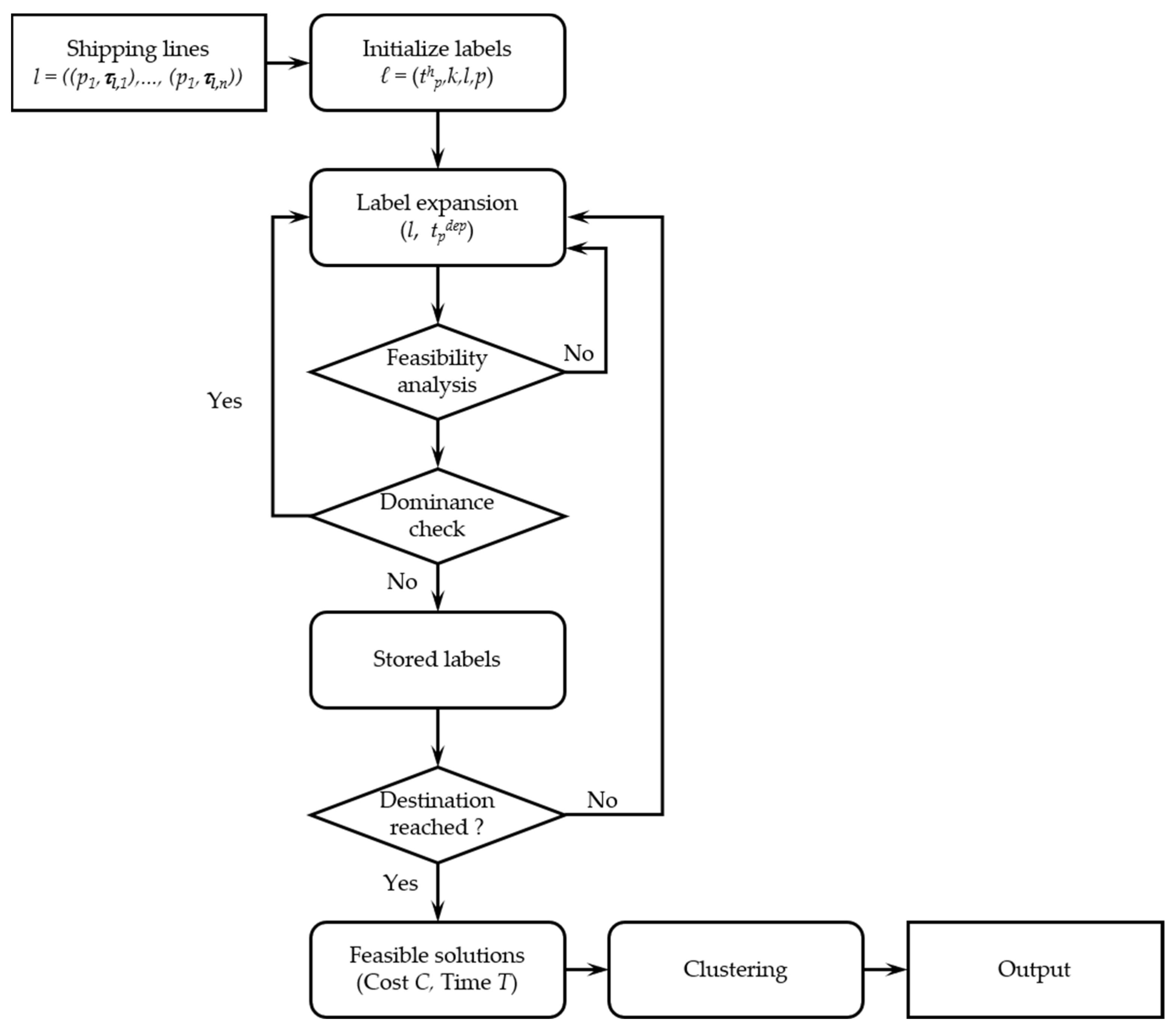
This section presents the routing methodology developed for liner shipping networks. The proposed approach explicitly enumerates feasible sequences of liner services and transshipment ports, evaluates their temporal feasibility, and identifies routing solutions with respect to total time and generalized cost. The approach is designed to guarantee structural feasibility, account for service schedules and operational constraints, and support comparative and exploratory analysis of routing solutions. Figure 1 reports the flowchart of the proposed procedure.

TACTIC adopts a label-setting approach to identify and store feasible routing solutions, ensuring both spatial and temporal feasibility in a maritime shipping network. The procedure takes as input the characteristics of the shipping lines l (ports and service schedules). A generic shipping line l is represented by an ordered sequence of port calls $l=\left((p_1,{\tau }_{l,1}),\dots ,(p_n,{\tau }_{l.n})\right)$, where p_i is port i and ${\tau }_{l,i}$ the vector containing the instants of arrival at port i (it is a vector whose components ${\tau }_{l,i}^{(m)}$ indicate that each line consistently reaches the port m times in the simulation window with its frequency f_l). For each container h, a label ℓ = (t^h_p,k,l,p), containing information on the arrival time t^h_p at port p with the service l, and the number of transshipments k, is initialized in the port of origin (in this case, k = 0). Afterwards, new labels are generated from each active label, considering sailing and waiting activities according to the available service (label expansion). Each label is first evaluated against temporal constraints and transshipment limits (feasibility analysis). Labels that violate these constraints are discarded, and the algorithm returns to the expansion phase. Feasible labels are subjected to a dominance check, whereby dominated labels are eliminated and non-dominated labels are stored for further expansion. For each stored label, the procedure verifies whether the destination port was reached. If the destination has not been reached, the expansion process is repeated; otherwise, the solution is deemed feasible and stored for a post-processing phase during which the solutions are selected following some criteria on time and cost. Finally, origin–destination pairs are clustered to generate routing profiles, which constitute the final outputs of the procedure.

In the following paragraphs, the procedure is explained in more detail.

At the topological level, an origin–destination pair of ports (p_o,p_d) can be connected through a sequence of services l, regardless of time and cost. Consequently, a feasible topological route (i.e., a sequence of ports and services) between two ports exists if topological connectivity exists, whereas a lack of topological connectivity is a cause of infeasibility. Temporal routing introduces operational realism and may invalidate topologically feasible solutions due to schedule misalignment or transshipment constraints. Given a topologically feasible pair (p_o,p_d), the time-dependent routing problem aims at identifying feasible and efficient routes considering schedules, waiting times, and transshipment constraints. In this context, the proposed procedure distinguishes between two types of infeasibilities:

• Topological infeasibility, which occurs when no admissible sequence of liner services can be identified between p_o and p_d;
• Schedule-related infeasibility, which occurs when a topological solution exists but cannot be transformed into a valid route due to schedule incompatibilities, or transshipment constraints (when the number of transshipments exceeds the maximum allowable threshold).

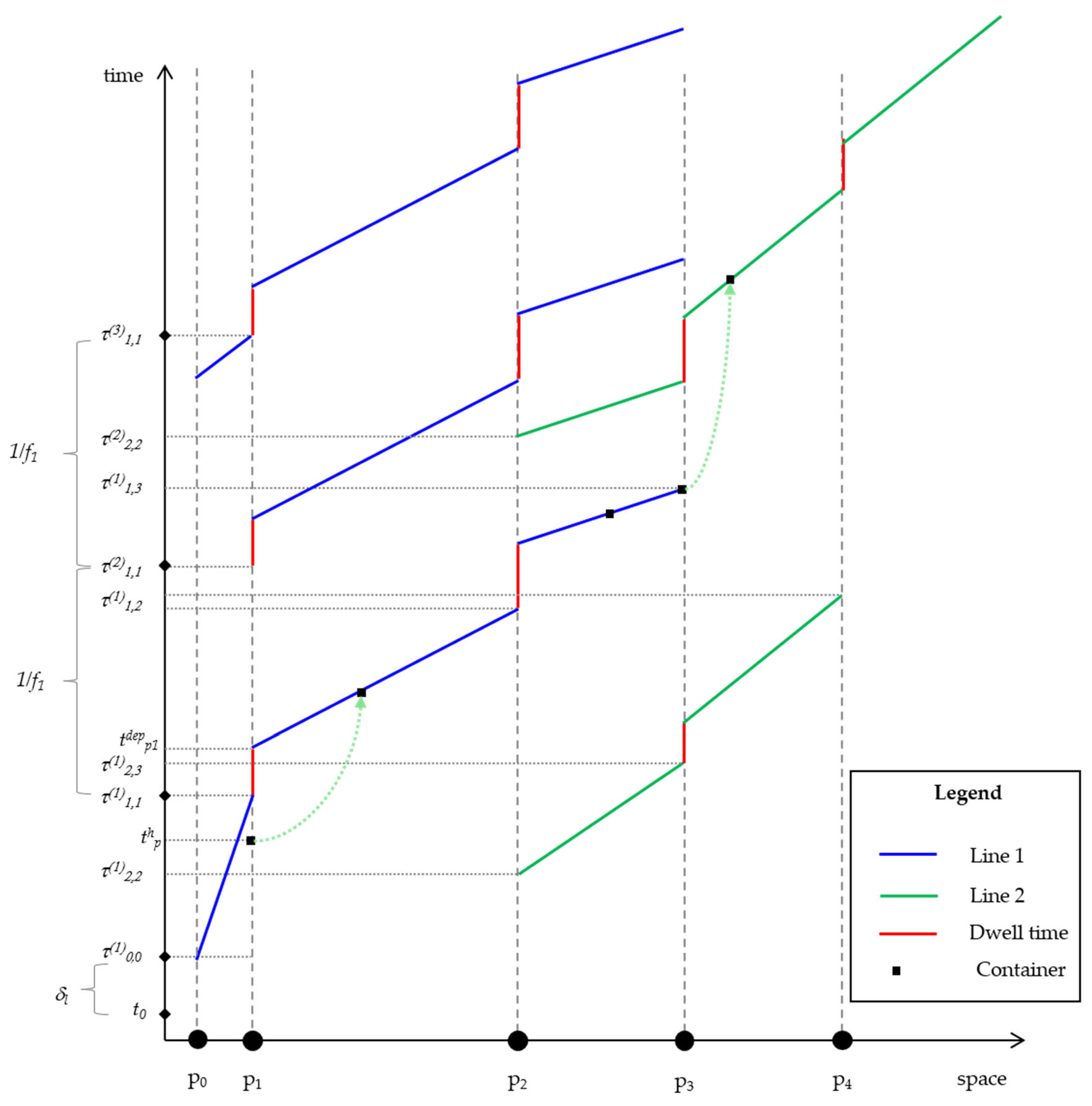
Figure 2 shows a simple case with two shipping lines. Line 1 operates between port 0 and port 3, while Line 2 operates between port 2 and port 4. Line 1 leaves from port 0 at t⁽¹⁾_1,0 (where (1) indicates that it is the first run of this line). In addition, each line has a frequency f_l and, assuming a regular service, two successive runs are spaced apart by a time equal to 1/f_l. Given a reference time t₀, the starting time of the first run will generally be d_l away from t₀. A generic container h embarks on Line 1 at port 1, continues to port 3, and then transfers (suffering a waiting time) to Line 2 to its destination.

The problem is solved using a label-setting algorithm, and each label is extended according to the route of the container; then, from a label ℓ at port p, feasible extensions are generated by selecting a service l at p, identifying the earliest feasible run of the line, and, finally, calculating the departure time of the container as:

$$t_p^{dep,h}={\displaystyle \frac{m^{\ast }}{f_l}}+T_p^d$$

where

• ${\displaystyle \frac{m^{\ast }}{f_l}}$ identify the earliest run of the line l;
• $T_p^d$ is the dwell time of the ship at port.

The value of m* is identified considering the constraint on the arrival time of the container h at port p:

$$t_p^h\le {\displaystyle \frac{m}{f_l}}+{\delta }_l+\lambda$$

where l is a constant value representing the minimum time required to complete the terminal operations preliminary to loading.

The value of m* is:

$$m^{\ast }=⌈f_l·(t_p^h-{\delta }_l-\lambda )⌉$$

Service changes increase the transshipment counter and are discarded if k > k_max. All non-dominated labels reaching p_d define feasible temporal routes. If no label reaches the destination, the instance is classified as temporally infeasible. For each feasible route, it is possible to calculate the sailing time T_s and the waiting time T_w, assumed as the sum of all the waiting times experienced by the container (waiting for loading at the first port, waiting times at intermediate ports, and any other waiting times related to transshipment operations). The value T = T_s + T_w is the total time of the solution. Finally, the total generalized cost is computed as follows:

$$C={\beta }_s·T_s+{\beta }_w·T_w+{\displaystyle \sum _{p\in Q}{\alpha }_p^h·c_p^h}$$

where

• b_s and b_w are homogenization coefficients;
• $c_p^h$ is the handling cost;
• ${\alpha }_p^h$ is a binary variable, equal to 1 if the container h is involved in a transshipment operation at port p, and 0 otherwise.

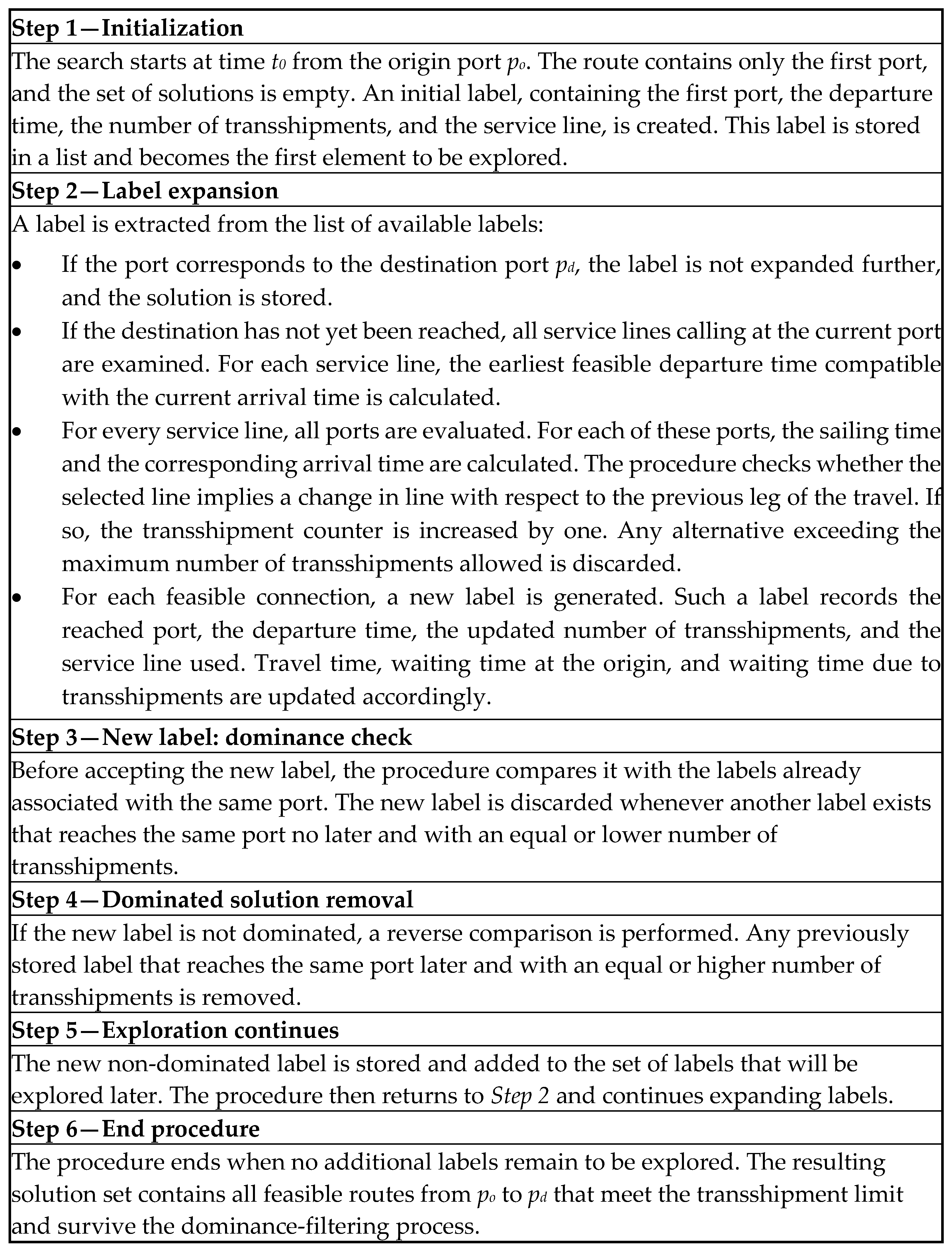
The proposed route-generation procedure (Figure 3) explores the maritime service network to identify all feasible routes between an origin port p_o and a destination port p_d. Given a departure time t₀ and the maximum number of allowable transshipments k_max, the procedure progressively constructs route alternatives by expanding feasible sailing connections and tracking the operational characteristics of each partial route. To ensure computational efficiency, dominated alternatives are discarded through a dominance mechanism based on arrival time and number of transshipments. The procedure terminates when no further route expansions are possible, returning the complete set of non-dominated feasible routes connecting p_o and p_d.

It should be noted that schedule offsets, sailing time, waiting time components, dwell time, and handling costs are treated as exogenous parameters within the proposed framework. Their values can be defined according to the application context and the availability of operational data. For computational experiments, parameter values were derived from the literature to ensure a controlled and comparable testing environment.

4. Case Study Description

4.1. Dataset

All calculations were carried out using publicly available data in order to make them replicable and comparable. In particular, the lines of the OCEAN Alliance (CMA CGM, Evergreen Line, Cosco Shipping, and OOCL), operating in the Mediterranean Sea and available at the CMA CGM online schedules [67], have been taken into account. To build the database, the report Main Lines by trade provided by CMA CGM [67] has been used. The report contains comprehensive information on service names, types, frequencies, vessel fleets, ports of call, day of call, and transit durations. Since the format of this source is not compatible with the main tools available for analysis, an extraction of the needed data (Supplementary File S1) and a data review were performed using a Python (version 3.11) script.

Table 1. Example of available data for intra-Mediterranean routes ⁽*⁾.

Service Name	SSLMED Euronaf loop Alger		SSLMED Euronaf loop Annaba Djen Djen
Service Code	ALGA		ALGAD
Fleet Size	3 ships (up to 889 TEU)		2 ships (up to 1118 TEU)
Operator	CMA-CGM		CMA-CGM
Frequency	Every week		Every week
Rotation duration [days]	21		14
Schedule & Transit Time	Location	Time	Location	Time
	Napoli	0	Barcelona	0
	La Spezia	1	Malta Freeport	2
	Genoa	2	Djen Djen	7
	Marseille	5	Barcelona	13
	Alger	8
	Napoli	19
Updated on	January 26		August 25

⁽*⁾ authors’ elaboration on data from [67].

shows an example of available data related to two intra-Mediterranean routes operated by CMA-CGM.

It is worth noting that, although the database thus constructed is not exhaustive of all connections (other operators are available in the area), as it is based on the lines operated by a single alliance, it is well suited to be used as an example of a real-world demonstration.

4.2. Application

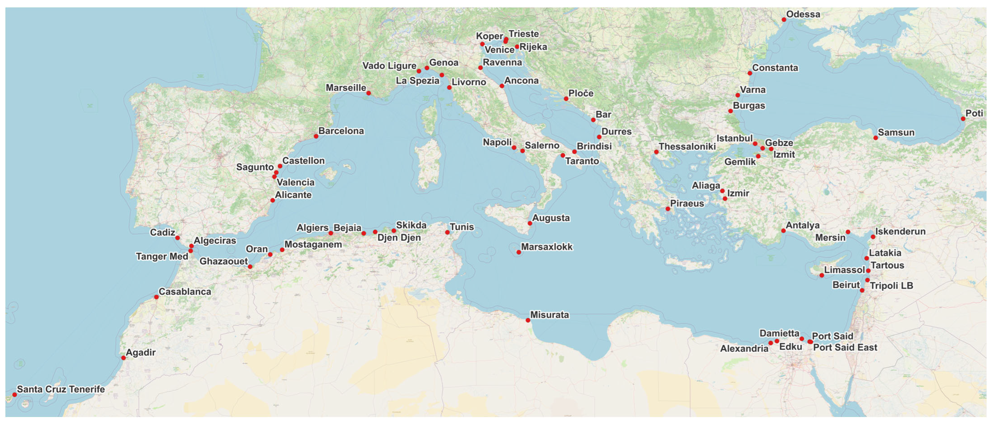
The test network consists of lines operating within the Mediterranean basin and its immediate surroundings (Figure 4). The covered ports are located mainly in Southern Europe, North Africa, and the eastern Mediterranean, including connections to the Black Sea and Levant areas. The ports considered are 64, for a total of 4032 origin–destination pairs covered by 48 shipping lines. This network does not include intercontinental routes, and it emphasizes short/medium-distance routes with a higher incidence of transshipment within the Mediterranean.

In route search, two criteria are considered: total travel time and total generalized cost. The maximum number of transshipments allowed is set to six, and the reference start day is fixed to day one. This means that the routing procedure is executed for a specific starting day and, to align departures and arrivals with actual schedules, the offset δ_l is associated with each shipping line l, allowing the search to reflect the temporal phase of each service. Moreover, for each port, to enhance the realism of the experiment, the dwell time $T_p^d$ and the cost associated with cargo handling at the port ($c_p^h$) are introduced. These assumptions ensure that the generated solutions are feasible and account for port-level operational characteristics, thereby providing more accurate time and cost estimates for the considered o-d pairs. For each origin–destination pair, the algorithm identifies all feasible routes that meet the topological and operational constraints. Among these, two reference solutions are extracted: the solution minimizing total travel time (best-in-time) and the solution minimizing total generalized cost (best-in-cost). As reported in Figure 3, the procedure generates feasible solutions with respect to the time constraints and retains only the non-dominated ones. Dominated solutions are discarded and excluded from further consideration. Since both time and cost components are non-negative, any extension of a dominated label cannot generate a route with a lower generalized cost than the corresponding route generated by extending the dominating label under the adopted cost structure. Among the non-dominated solutions, the route with the minimum total time and the route with minimum cost (total time and cost component are defined in Section 3) are selected.

These parameters are summarized in

Table 2. Operational and cost parameters used in computational experiments.

Parameter	Value
Maximum number of transshipments (kmax)	6
Start day	1
bs [EUR/h/TEU]	1.0625 (*) [69]
bw [EUR/h/TEU]	1.417 (*) [69]
$c_p^h$ [EUR/TEU]	100 (**) [70,71]

⁽*⁾ 1 $ = 0.85 €; ⁽**⁾ value within the range defined in the literature.

.

To preserve modularity, routing outputs are post-processed without altering the optimization engine. The post-processing phase ensures:

• Consistency between service changes and transshipment ports;
• Coherent, compact, and detailed route representations.

5. Discussion

5.1. Routing Outcomes

To gain insight into the characteristics of the computed routes, aggregate statistics are derived separately for best-in-time and best-in-cost solutions. For each type of solution, the average values are calculated for total travel time, waiting components, navigation time, generalized cost, and number of transshipments. These aggregated indicators are reported in

Table 3. Indicators for best-in-time and best-in-cost solutions.

Indicator	Best-in-Time	Best-in-Cost	Δ (*)
Total travel time [h]	352.74	371.72	−5.38%
Waiting time at origin [h]	5.91	6.10	−3.21%
Waiting time at transshipment [h]	47.97	35.22	26.58%
Navigation time [h]	298.87	330.40	−10.55%
Total cost [EUR/TEU]	467.97	441.73	5.61%
Navigation cost [EUR/TEU]	204.09	223.25	−9.39%
Waiting cost [EUR/TEU]	87.35	76.86	12.01%
Handling cost [EUR/TEU]	176.54	141.61	19.79%
Number of transshipments	1.77	1.42	19.77%

⁽*⁾ best in time vs. best in cost.

, which provides a compact overview of the routing patterns emerging under different optimization criteria. The indicators reported include the total travel time, the waiting times at the origin and at the transshipment, the navigation time, the total cost (and its breakdown), and the average number of transshipments. The waiting times at the origin are similar in the two optimization criteria, suggesting that the choice of objective has little influence on initial port scheduling. However, the waiting time for transshipment and handling cost varies more substantially (26.58% and 19.79%, respectively). Table 3 provides a comparison between the indicators obtained under the optimization criteria (the variation is calculated with respect to the best-in-time indicators). As expected, the percentage variation in time is negative, except for the one related to the transshipment (this happens because the minimization of costs leads to the reduction in the number of transshipment operations). Similarly, the percentage variation in costs is positive except for the one related to navigation (this happens because navigation time is always lower in best-in-time solutions).

Beyond the numerical comparison, the observed differences between the best-in-time and best-in-cost solutions suggest operational implications for stakeholders in maritime transport. The reduction in total travel time achieved by best-in-time solutions indicates a preference for faster services and route combinations. From an operational perspective, this suggests that network planners aiming to improve service responsiveness may prioritize connections with higher frequencies or shorter maritime legs, even when these options involve additional intermediate transshipments. In fact, when comparing best-in-time and best-in-cost solutions, the average number of transshipments increases (from 1.42 to 1.77). Then, in the best-in-time solutions, the container is transferred more frequently across intermediate ports to take advantage of faster lines. While this strategy reduces navigation time by 10.55%, it also leads to a 26.58% increase in transshipment waiting time and a nearly 20% increase in handling costs. These results underline that time savings are achieved with penalties: additional port operations create extra handling requirements and expose shipments to greater dependence on terminal efficiency and synchronization between services. On the contrary, the best-in-cost solutions show that lower transport costs are obtained by reducing the number of transshipment operations. From an operational standpoint, this corresponds to selecting more direct service lines, even when they involve longer sailing times. Fewer transshipments not only reduce handling costs, but also reduce the operational complexity associated with container transfers between services.

These findings provide useful guidance for port managers and route planners. Port managers could use the results to improve the efficiency of transshipment, increasing the attractiveness of the port. For route planners, the results indicate a trade-off between service speed and operational simplicity: achieving shorter delivery times requires more transshipment activities, whereas minimizing costs favors routes with fewer intermediate operations. Therefore, the choice between the two optimization criteria should be viewed as a strategic decision about the design of the network that reflects different operational priorities rather than simply a numerical difference in time or cost indicators.

5.2. Cluster Analysis

The aim of the cluster analysis is to group o-d pairs with similar indicators related to the container routing. In order to identify the clusters, a principal components analysis [72] was performed, with the aim of obtaining the directions of maximum variability and reducing the effect of noise. Due to the relationships between the variables reported in Table 3, several indicators (e.g., total travel time and total cost) can be expressed as linear combinations of more elementary components. Therefore, to avoid redundancy and multicollinearity, the principal components analysis was performed only on the fundamental variables (waiting time at origin, waiting time at transshipment, and navigation time), which form the basis of the other derived indicators.

Since the routing results refer to two different criteria (time and cost), the Kaiser test, needed to identify the principal components, is repeated twice. In the case of best-in-time solutions, the Kaiser test indicated that the first two principal components (PCs) have eigenvalues greater than 1 (PC1 = 1.232, PC2 = 1.072), while the third component (PC3 = 0.697) is less significant. Therefore, the first two components, which explain most of the overall variability in the data, were retained. The principal components appear to be linear combinations of the original variables: the first component (PC1) is associated with waiting times at origin and navigation (factors equal to 0.72 and 0.69, respectively), while the second (PC2) is influenced by waiting times in transshipment (with a factor equal to 0.89). Similar considerations are given for the best-in-cost case, where the first two components are significant. The first component (PC1) is associated with waiting times at origin and navigation (factors equal to 0.69 and 0.57, respectively), while the second (PC2) is influenced by waiting times in transshipment (with a factor equal to 0.80) and navigation time (0.60).

The number of clusters k was determined through a joint evaluation of the silhouette coefficient [73] and the analytical elbow criterion (SSE) supported by a curvature-based detection rule [74]. The elbow method captures the global reduction in within-cluster variance, whereas the silhouette score assesses the separation and cohesion of the resulting partition. Given the correlated nature of our operational indicators, the silhouette measure provides essential evidence on whether a partition corresponds to meaningful behavioral groups. When the two diagnostics provide different values, low silhouette scores (e.g., s(k) < 0.35) are interpreted as indicating poorly separated clusters, and such values of k are excluded. In line with a conservative modeling approach, the final choice is therefore set to k = min(ksilhouette, kelbow), ensuring that the resulting clusters remain interpretable and consistent with the routing profiles considered in the analysis.

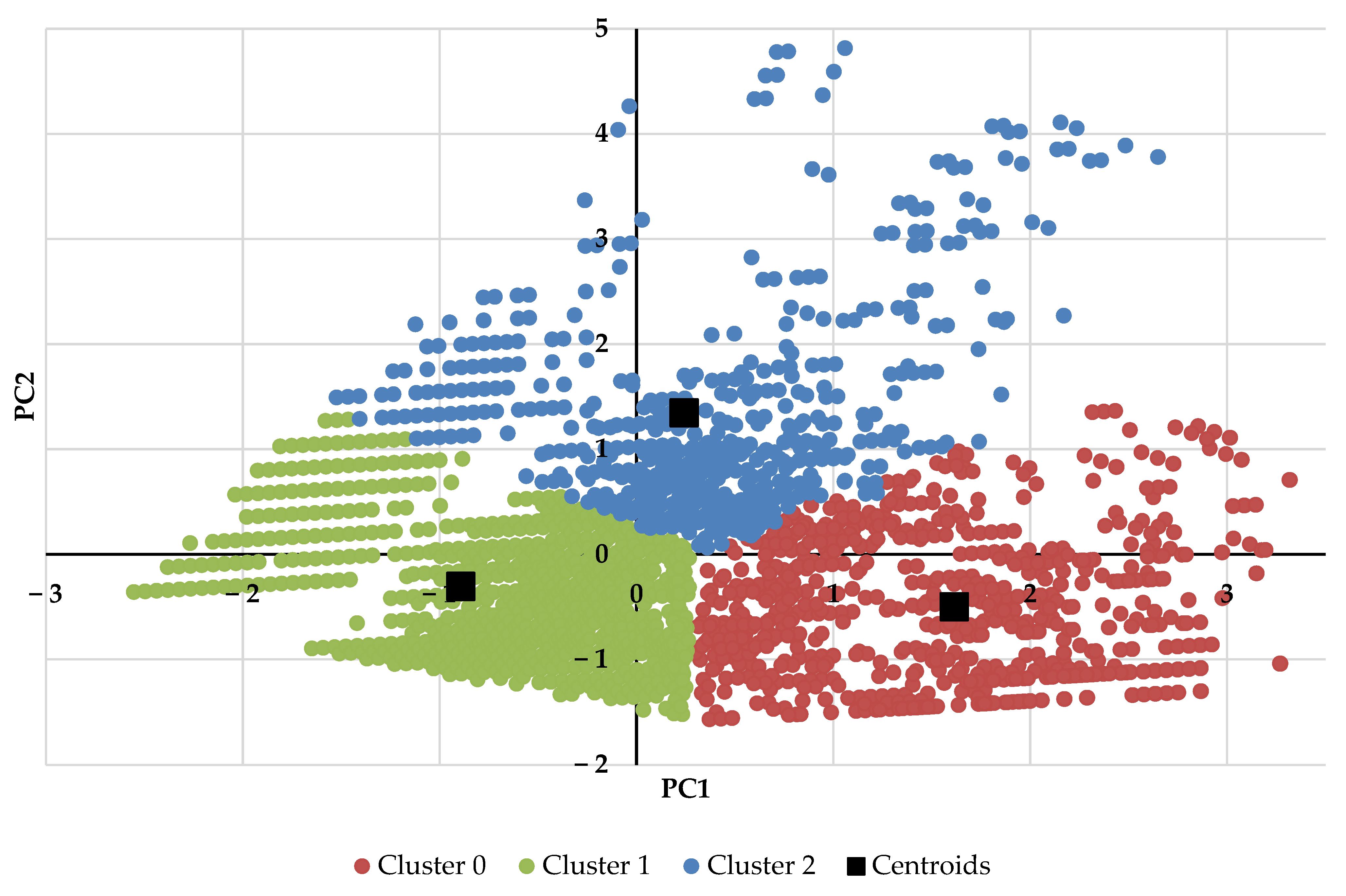
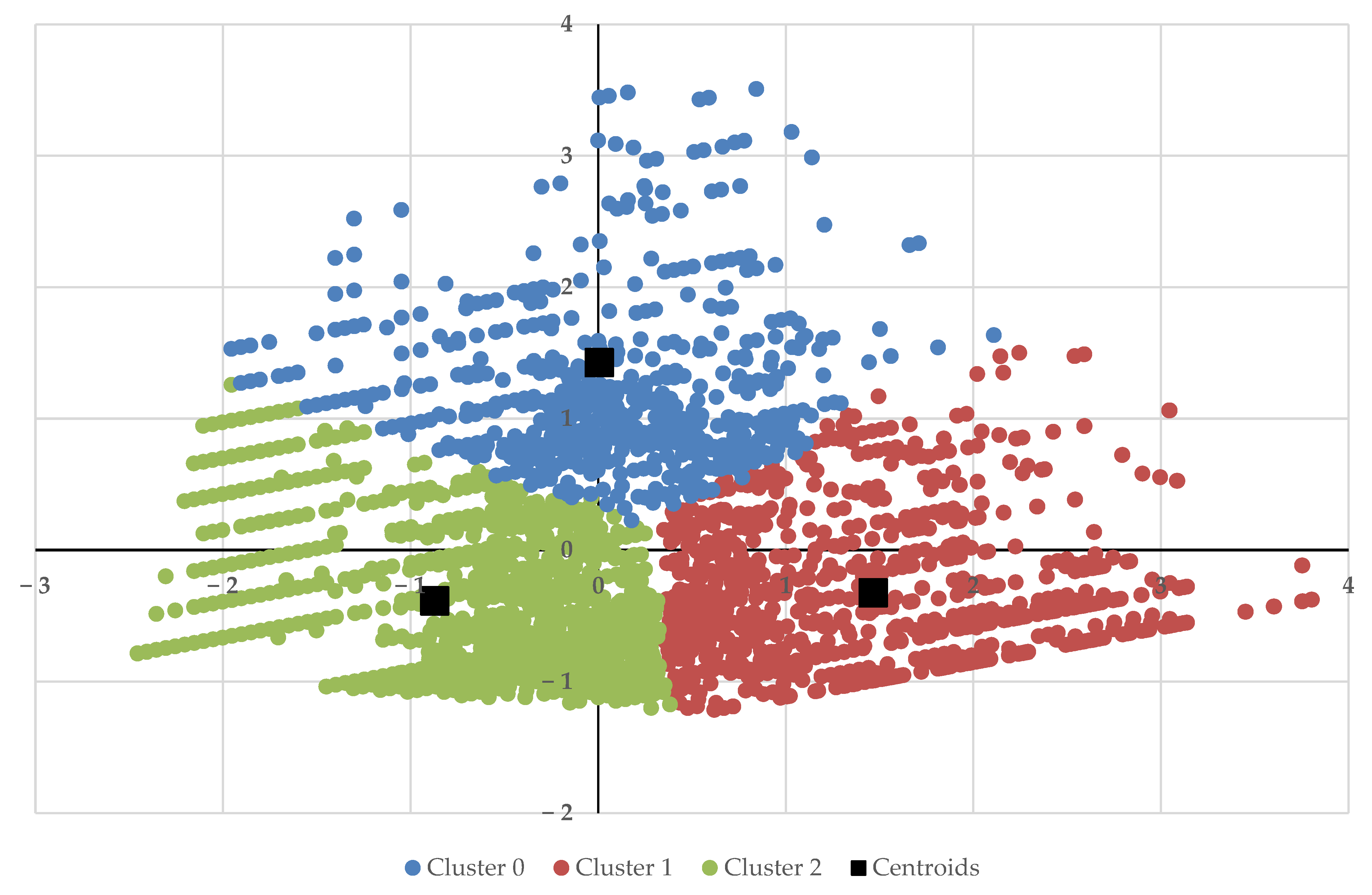
Figure 5 and Figure 6 show the results of applying the k-means algorithm to the space of the first two principal components. In both representations, three distinct groups of observations emerge.

In Figure 5, the first principal component (PC1) distinguishes cluster 0, located in the region with high positive values from cluster 1, which occupies the negative side of the axis. Cluster 2, instead, is separated along the second principal component (PC2), as it is concentrated in the upper region with positive values. Some overlaps are observed in the central areas, particularly between cluster 2 and the other two clusters, indicating a gradual transition between observations.

In Figure 6, the cluster structure is still identifiable, but with a less clear separation than in the previous case. The first principal component (PC1) still provides the main axis of discrimination, separating the cluster located in the positive region from the one occupying the negative side of the axis. However, cluster 0 is concentrated in the central region and extends toward higher values along the second principal component (PC2), contributing to a substantial overlap among clusters. In particular, a high density of observations is located around the origin, where all three clusters partially intersect, indicating a less distinct partition and a more gradual transition between groups.

Table 4. Resuming cluster characteristics: best-in-time solutions.

Indicator	Cluster 0	Cluster 1	Cluster 2
Number of o-d pairs	1007	2181	844
Share of total o-d pairs [%]	24.98	54.09	20.93

and

Table 5. Resuming cluster characteristics: best-in-cost solutions.

Indicator	Cluster 0	Cluster 1	Cluster 2
Number of o-d pairs	819	1196	2017
Share of total o-d pairs [%]	20.31	29.66	50.03

report the number of o-d pairs belonging to each cluster, highlighting the balance across clusters.

The proposed clustering approach can support decision-makers’ decisions related to container transport. Grouping o-d pairs with similar cost and travel time characteristics into a limited number of homogeneous categories allows planners to use these clusters as representative operational segments when evaluating transport services and network configurations. From a service planning perspective, identified clusters can support the prioritization of interventions and investments. The o-d pairs grouped within a cluster exhibit similar responses to modifications in network design, routing strategies, transshipment structures, or terminal operations. Consequently, planners can assess the potential benefits of specific measures at the cluster level before analyzing each o-d pair in detail. This reduces the complexity of decision-making when a large number of transport o-d pairs are involved.

The clustering results can also be used as a benchmarking tool. By comparing the centroid of each cluster with the characteristics of each o-d pair, decision-makers can identify routes that perform significantly worse than the typical cost–time trend of their group. These routes may deserve further investigation to identify the causes of inefficiency (e.g., bottlenecks) and solve them.

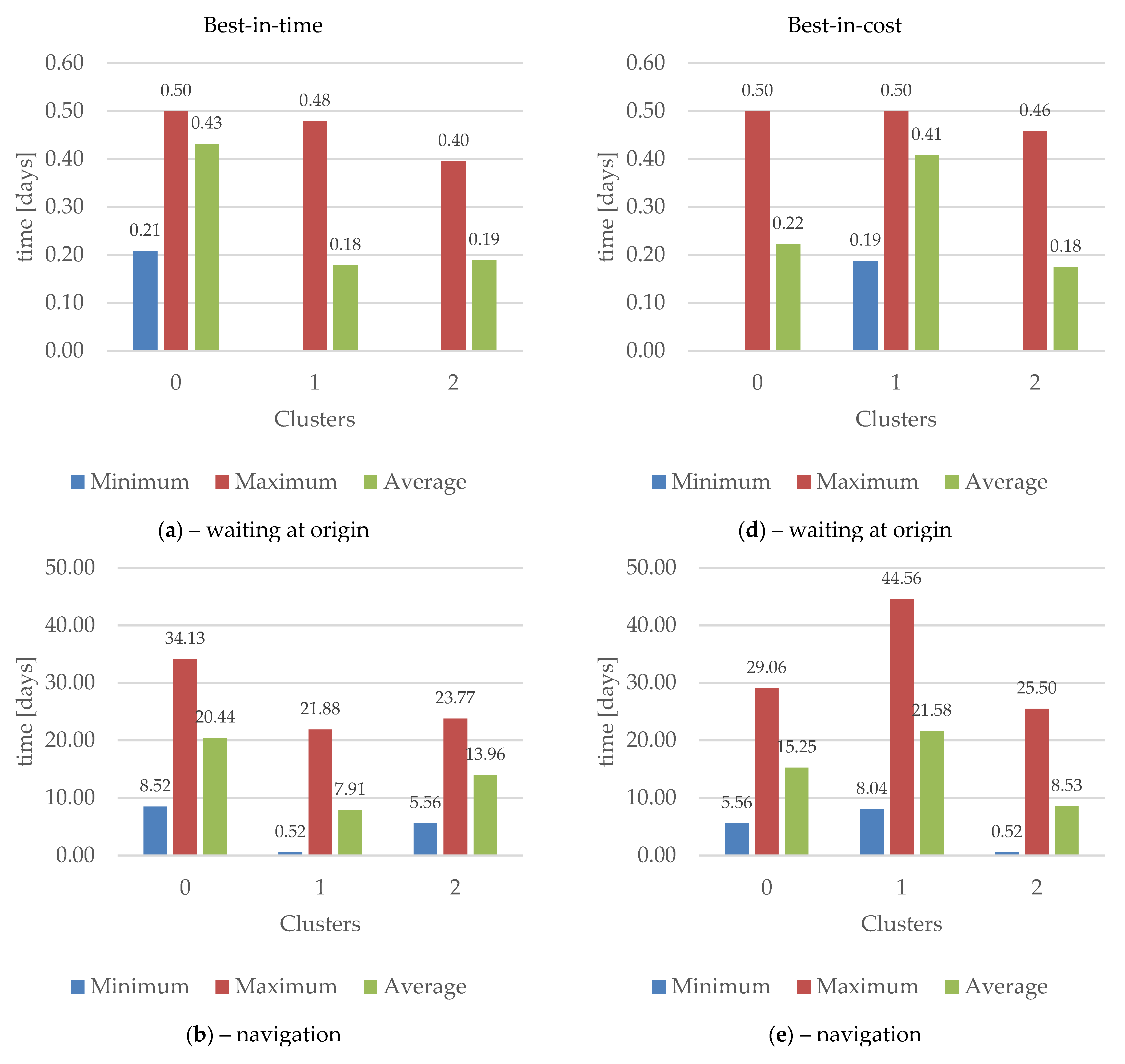
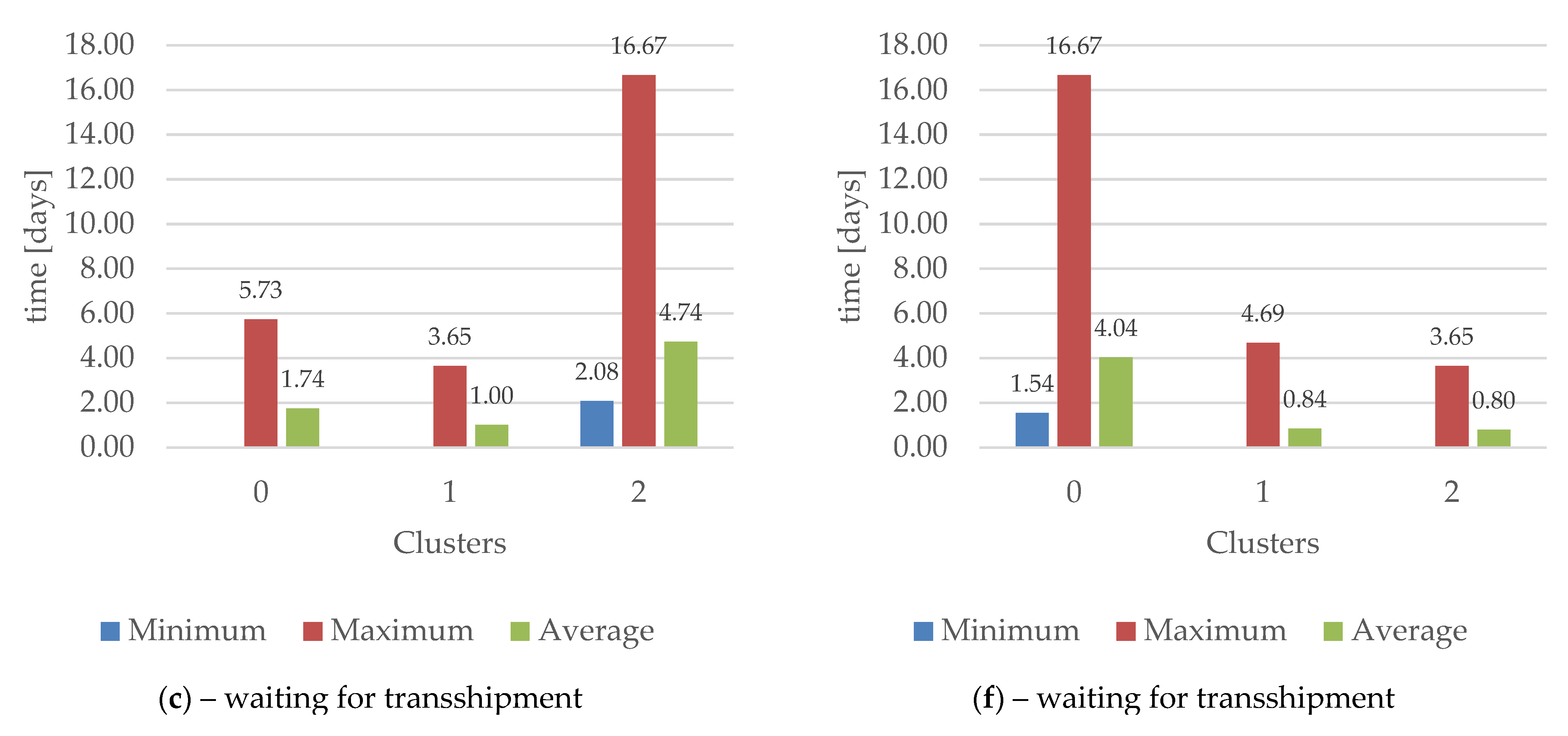
Figure 7 reports the main descriptive statistics of the original variables (waiting time at origin, navigation time, and waiting time for transshipment) for each cluster identified. This analysis allows for a more interpretable characterization of the clusters that emerged in the principal components space.

Focusing on the best-in-time solutions, the waiting time at the origin highlights a clear distinction between cluster 0, which has a higher average value (0.43 days), and clusters 1 and 2, which have low and comparable average values (0.18 and 0.19 days, respectively). A similar trend is observed for navigation time: cluster 0 has the highest average value (20.44 days), followed by cluster 2 (13.96 days), while cluster 1 stands out for its lowest average value (7.91 days). Regarding the waiting time for transshipment, a distinct pattern emerges; in fact, cluster 2 presents the highest average value (4.74 days), while clusters 0 and 1 show lower average values (1.74 and 1.00 days, respectively). In summary, referring to average values, cluster 0 presents high values in terms of waiting time at origin and navigation, but it is characterized by a low waiting time for transshipment. Cluster 1 contains the o-d pairs with the shortest navigation time and lowest levels of wait for transshipment. Cluster 2 presents high values of both the waiting time for transshipment and the navigation time, making it the group of o-d pairs with the worst time, despite a lower waiting time for transshipment.

Focusing on the best-in-cost solutions, and in relation to the waiting time at the origin, clusters 0 and 2 present similar average values (0.22 and 0.18 days), while cluster 1 has a higher average value (0.41 days). This result highlights how cluster 2 groups o-d pairs, for which the operating conditions are penalized in the initial phase of the routing. Regarding navigation time, cluster 1 contains those o-d pairs for which the average travel time is about 21 days. Cluster 0 shows a decrease in the average travel time (15.25 days), which continues to decrease for the pairs in cluster 2 (8.53 days). In the case of waiting time for transshipment, the o-d pairs in cluster 0 have an average value of 4.04 days, while clusters 1 and 2 show much lower and similar values (0.84 and 0.80 days, respectively). In summary, cluster 0 shows intermediate values of navigation time and low waiting times at origin, but it is distinguished by a high waiting time for transshipment. Cluster 1 presents high average values both in waiting time at the origin and in navigation time despite having short transshipment times. Cluster 2 is the one with the shortest average times in all phases and, in particular, has the shortest navigation time and the lowest waiting levels in transshipment.

5.3. Comparison with Other Algorithms

The proposed approach has been compared with other algorithms on the basis of the results obtained for two other representative networks (named network A and network B) with different sizes and complexities adopted in [75]. Such algorithms are the connection scan algorithm (CSA) and RAPTOR [76,77]. Network A is constructed by selecting six liner services that connect the Mediterranean area with extra-Mediterranean regions. Network B is the largest one, encompassing all lines included in the dataset. This network represents a highly connected global routing scenario, intended to stress-test the routing algorithm under realistic and large-scale operational conditions.

Table 6. Routing outcomes averaged over all origin–destination pairs for network A.

Indicator	CSA	RAPTOR	TACTIC Best-in-Time	TACTIC Best-in-Cost	TACTIC Best-in-Time/CSA	TACTIC Best-in-Time/RAPTOR	TACTIC Best-in-Cost/CSA	TACTIC Best-in-Cost/RAPTOR
Average time in hours	2194.90	1789.90	1592.73	1598.77	−27.43%	−11.02%	−27.16%	−10.68%
Average no. of transshipments	2.21	1.15	1.23	1.20	−44.34%	6.96%	−45.70%	4.35%
Maximum no. of transshipments	5	3	3	3	−40.00%	0.00%	−40.00%	0.00%

and

Table 7. Routing outcomes averaged over all origin–destination pairs for network B.

Indicator	CSA	RAPTOR	TACTIC Best-in-Time	TACTIC Best-in-Cost	TACTIC Best-in-Time/CSA	TACTIC Best-in-Time/RAPTOR	TACTIC Best-in-Cost/CSA	TACTIC Best-in-Cost/RAPTOR
Average time in hours	1495.70	1435.80	1265.00	1339.90	−15.42%	−11.90%	−10.42%	−6.68%
Average no. of transshipments	5.56	2.57	2.82	2.24	−49.28%	9.73%	−59.71%	−12.84%
Maximum no. of transshipments	15	9	9	7	−40.00%	0.00%	−53.33%	−22.22%

summarize the main routing indicators averaged over all origin–destination pairs for the four procedures (CSA, RAPTOR, TACTIC (best-in-time), and TACTIC (best-in-cost)) in both networks.

In network A, CSA produces the worst performance in terms of travel time, with an average travel time of 2194.90 h, compared with 1789.90 h for RAPTOR. Both TACTIC variants further improve the results, reducing the average travel time to 1592.73 h for the best-in-time solution and 1598.77 h for the best-in-cost solution. This corresponds to a reduction of approximately 27% with respect to CSA and about 11% with respect to RAPTOR. Similar trends emerge for the number of transshipments. CSA generates almost twice as many transfers on average (2.21) as RAPTOR (1.15), while the two TACTIC variants maintain values very close to RAPTOR (1.23 for best-in-time and 1.20 for best-in-cost). The maximum number of transshipments is also lower for RAPTOR and both TACTIC procedures (three) than for CSA (five), indicating that these approaches are more effective at reducing route complexity.

The same pattern is observed in network B, although the differences become even more pronounced. CSA again yields the highest average travel time (1495.70 h), while RAPTOR achieves a modest improvement (1435.80 h). The best performance is obtained by TACTIC best-in-time, with an average travel time of 1265.00 h, followed by TACTIC best-in-cost with 1339.90 h. Compared with CSA, the reduction in travel time reaches about 15% for TACTIC best-in-time and 10% for TACTIC best-in-cost.

Regarding transshipment, CSA produces the larger number of transshipments, with an average value of 5.56, more than double that obtained with RAPTOR (2.57). The TACTIC procedures reduce this indicator as well, with averages of 2.82 for best-in-time and 2.24 for best-in-cost approach. Notably, TACTIC best-in-cost provides the best trade-off, combining a significant reduction in travel time with the lowest average number of transfers. This result is confirmed by the maximum number of transshipments, which has the lowest value corresponding to the best-in-cost solution.

Overall, the results show that the TACTIC approaches outperform both CSA and RAPTOR in terms of travel time while maintaining a limited number of transshipments.

5.4. Sensitivity Analysis and Scalability

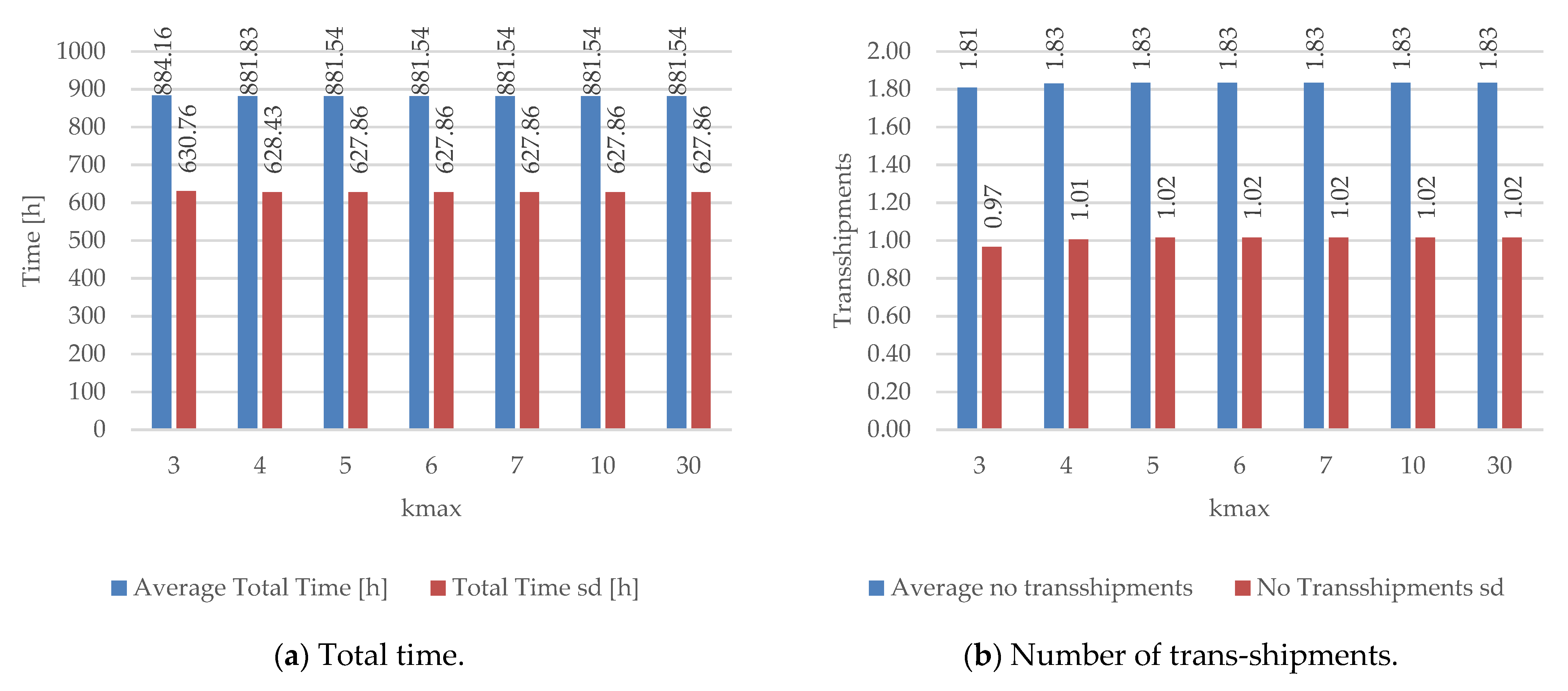
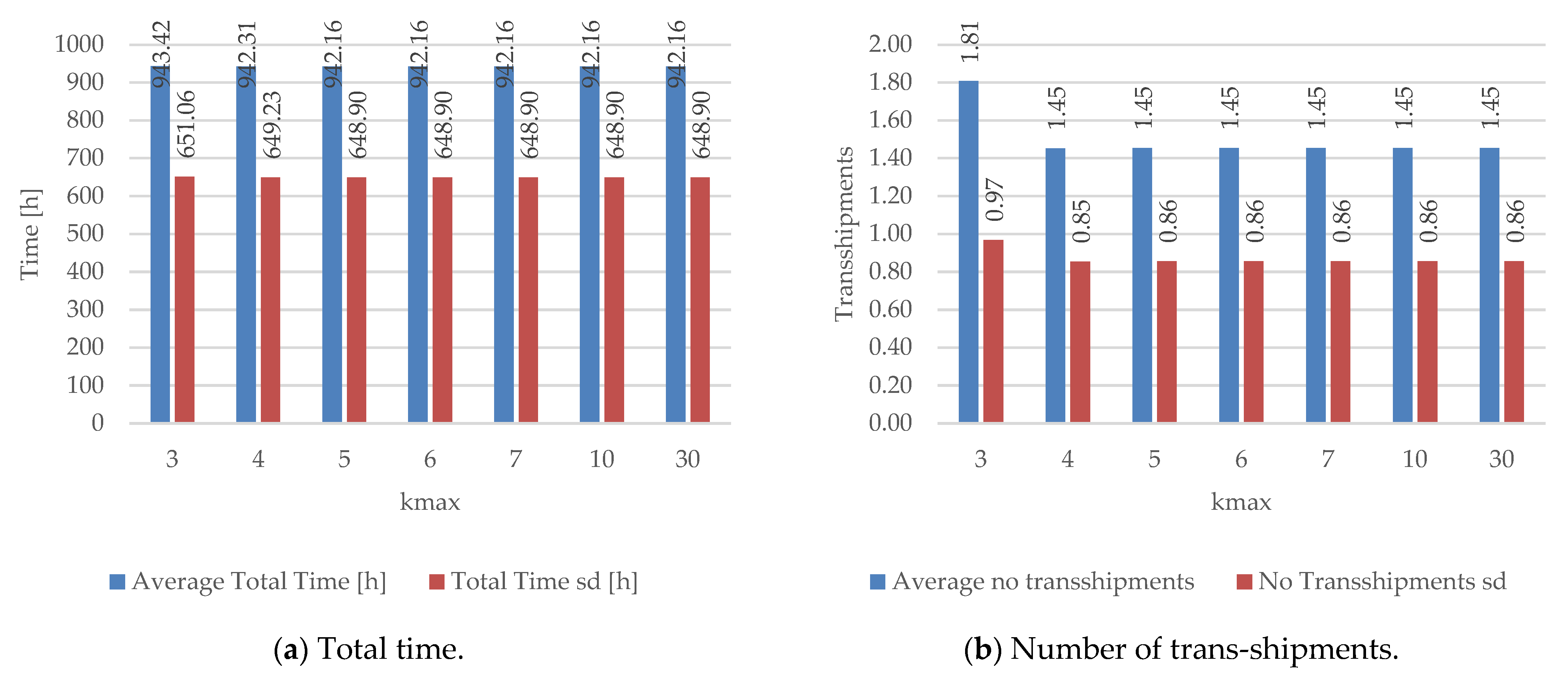
The results provided in the previous sections depend on the value of the parameters used in the procedure (Table 2). This implies that a variation in the value of the parameters affects the results, both in terms of time and cost. Considering that the parameters related to the costs are from the literature, an analysis of the impact of the maximum number of transshipments allowed (k_max) is performed. The indicators used are the average and the standard deviation of the total time T and the average and standard deviation of the number of transshipments. Figure 8 and Figure 9 show the results obtained for both approaches; the most significant variations are observed when k_max increases from 3 to 5, while no appreciable changes occur for larger values. This behavior suggests that the majority of feasible routes require at most five transshipments and that the network connectivity is sufficiently high to guarantee access to the best solutions without allowing an excessive number of intermediate transfers.

To investigate the variability of the TACTIC’s runtime as the number of ports or service lines increases, the test network and the two other representative networks described in the previous point have been considered.

Table 8. Computational performance of the procedure on the three representative networks.

Variable	Network A	Test Network	Network B
Ports	47	64	416
Services	6	48	313
o-d pairs	2162	4032	172,640
CPU time [s]	5.936	67.256	19,011.500
Avg. time per origin [s]	0.126	1.051	45.701

reports the computational performance of the proposed procedure on three representative networks characterized by increasing size and complexity. The analysis considers the number of ports, services, o-d pairs, total CPU time, and average computation time per origin.

As expected, the computational effort increases with network size. Network A, consisting of 47 ports and six services, requires only 5.936 s to process 2162 o-d pairs, corresponding to an average computation time of 0.126 s per origin. The test network, with 64 ports and 48 services, requires a computational time of 67.256 s for 4032 o-d pairs, while the average processing time rises to 1.051 s per origin.

The largest increase is observed for network B, which includes 416 ports and 313 services and generates 172,640 o-d pairs. In this case, the total execution time reaches 19,011.50 s, with an average computation time of 45.701 s per origin. The growth in computational effort is therefore more than proportional to the increase in network size, reflecting the larger search space and the much higher number of feasible route combinations that must be evaluated.

Nevertheless, the results demonstrate that the proposed procedure remains computationally tractable even for large-scale freight transport networks. Although the total execution time increases, the algorithm successfully processes a network involving hundreds of ports and services and more than 172,000 origin–destination pairs within a few hours. This suggests that the approach can support strategic and tactical planning activities, where route calculations are typically performed offline rather than in real time.

To frame the results obtained against the current literature,

Table 9. Comparing some existing methods with the proposed approach.

Reference	Objectives	Graph Representation	Pro and Cons
Wang et al. [11]	Manage contains flow	Service network	Minimum cost routes Scalability
Meng & Wang [78]	Optimize shipping services and container flows	Service network	Integrates design and flow allocation Computational complexity
Zhen et al. [79]	Emissions control; optimize routes and speed	Service network	Integrated decisions Computational complexity
LaRock et al. [80]	Analyzing liner shipping service routes	Route-based graph	Centrality measure Only topological
Zhang et al. [81]	Detect transshipment hubs	Service network	Focus on transshipment hubs No routing optimization
This paper	Optimize container routes	Service network	Tool to explore and classify routing patterns Not consider delay/disruption

compares some aspects of research on container shipping networks. Most studies focus on optimizing container flows and shipping services through service-network representations, with particular attention to cost minimization and fleet utilization. Other contributions expanded the objectives, including planning decisions, environmental considerations, and the analysis of network topology. In particular, route-based and complex-network approaches have improved the understanding of connectivity patterns and the role of transshipment hubs, although they generally remain descriptive rather than prescriptive. Despite the significant advances achieved by previous studies, limited attention has been devoted to the joint analysis of routing patterns, transshipment effects, travel times, and generalized transport costs within a unified framework. Furthermore, most existing studies either focus on optimization aspects or on network structure, while fewer contributions attempt to combine both perspectives in the analysis of container routing solutions.

6. Conclusions

This paper has presented a comprehensive framework for routing analysis in liner shipping networks that integrates temporal feasibility, cost evaluation, and a multi-criteria approach within a unified methodological structure. Unlike procedures relying solely on topological connectivity or static shortest-path formulations, the proposed framework explicitly incorporates service schedules, frequencies, dwell times, port-specific handling costs, and transshipment limits, ensuring the generation of operationally feasible routes. The results demonstrate that the procedure works for realistic shipping networks, while maintaining full coverage of origin–destination pairs. The comparison between best-in-time and best-in-cost solutions shows that, although average performance indicators may appear similar, a substantial share of o-d pairs exhibits structurally different routing characteristics. Beyond aggregate indicators, clustering analysis provides an interpretation of the solution space. Identification of distinct routing profiles reveals systematic patterns related to origin waiting times, transshipment, and multi-transshipment routes. These insights cannot be captured by single-objective routing approaches and are particularly relevant for strategic planning, service evaluation, and network diagnostics.

From a methodological perspective, the modular design of the procedure allows for straightforward extensions, including alternative cost structures, reliability considerations, capacity constraints, or scenario-based analyses. From an applied point of view, the framework supports the use of advanced routing analytics as an effective decision-support tool for liner shipping operators and policymakers.

From a practical perspective, the results suggest that the proposed procedures can improve the efficiency of freight transport planning. While the best-in-time approach achieves the greatest reduction in travel times, the best-in-cost approach provides the most balanced solution by combining competitive travel times with the lowest number of transshipments. Since each transshipment operation involves additional handling costs, resource utilization, and potential delay risks, the reduction in transfers achieved by TACTIC best-in-time may generate significant operational benefits. Consequently, the proposed methods appear to be particularly suitable for large-scale freight transportation networks, where improvements in routing efficiency can translate into lower logistics costs and more reliable supply chains. In addition, the results indicate that the proposed methodology scales with network size. While computation times increase significantly as the number of ports, services, and o-d pairs grows, the procedure remains applicable to realistic large-scale maritime freight networks, demonstrating its potential for practical deployment in complex intermodal logistics systems.

The proposed procedure is not without limitations. The first limitation concerns the application, specifically the fact that only one shipping operator was considered, while others operate in the area. The procedure could therefore be extended in the future to include all available services and their integration (this could be done by considering route data from automatic identification systems). Another limitation is related to the fact that it was assumed that the service works as scheduled, without delays or disruptions. To overcome this aspect, future research will focus on extensions to stochastic settings, incorporating schedule uncertainty and disruption risks, and applying the framework to real-world case studies involving competing service configurations and dynamic demand patterns.

References

1. Russo, F.; Musolino, G.; Assumma, V. An Integrated Procedure to Estimate Demand Flows of Maritime Container Transport at International Scale. Int. J. Shipp. Transp. Logist. 2014, 6, 112–132. [Google Scholar] [CrossRef]
2. Russo, F.; Musolino, G.; Assumma, V. Ro-Ro and Lo-Lo Alternatives between Mediterranean Countries: Factors Affecting the Service Choice. Case Stud. Transp. Policy 2023, 11, 100960. [Google Scholar] [CrossRef]
3. Lee, S.M.; Roh, M.I.; Kim, K.S.; Jung, H.; Park, J.J. Method for a Simultaneous Determination of the Path and the Speed for Ship Route Planning Problems. Ocean Eng. 2018, 157, 301–312. [Google Scholar] [CrossRef]
4. Zhao, W.; Wang, Y.; Zhang, Z.; Wang, H. Multicriteria Ship Route Planning Method Based on Improved Particle Swarm Optimization–Genetic Algorithm. J. Mar. Sci. Eng. 2021, 9, 357. [Google Scholar] [CrossRef]
5. Chen, X.; Hu, R.; Luo, K.; Wu, H.; Biancardo, S.A.; Zheng, Y.; Xian, J. Intelligent Ship Route Planning via an A∗ Search Model Enhanced Double-Deep Q-Network. Ocean Eng. 2025, 327, 120956. [Google Scholar] [CrossRef]
6. Russo, F.; Pedà, G.; Musolino, G. Attributes Influencing Port Times of Container Ships. WMU J. Marit. Aff. 2024, 23, 375–392. [Google Scholar] [CrossRef]
7. Russo, F.; Musolino, G. Transportation System Models to Analyse Ports Competition and Cooperation. WMU J. Marit. Aff. 2024, 23, 393–413. [Google Scholar] [CrossRef]
8. Musolino, G.; Panuccio, P.; Rindone, C.; Russo, F.; Vitetta, A. National and Local Factors Affecting Ship Time in Container Ports: System of Models at Country and Port Levels. In Proceedings of the Computational Science and Its Applications—ICCSA 2025 Workshops; Gervasi, O., Murgante, B., Garau, C., Karaca, Y., Faginas Lago, M.N., Scorza, F., Braga, A.C., Eds.; Springer Nature: Cham, Switzerland, 2026; pp. 144–155. [Google Scholar]
9. Musolino, G.; Panuccio, P.; Rindone, C.; Russo, F.; Vitetta, A. Analysis and Interpretation of Attributes Affecting Ship Time in Container Ports. In Proceedings of the Computational Science and Its Applications—ICCSA 2026 Workshops; Gervasi, O., Murgante, B., Garau, C., Rocha, A.M.A.C., Faginas Lago, M.N., Braga, A.C., Karaca, Y., Eds.; Springer Nature: Cham, Switzerland, 2026; pp. 543–555. [Google Scholar]
10. Karsten, C.V.; Ropke, S.; Pisinger, D. Simultaneous Optimization of Container Ship Sailing Speed and Container Routing with Transit Time Restrictions. Transp. Sci. 2018, 52, 769–787. [Google Scholar] [CrossRef]
11. Wang, S.; Meng, Q.; Sun, Z. Container Routing in Liner Shipping. Transp. Res. Part E Logist. Transp. Rev. 2013, 49, 1–7. [Google Scholar] [CrossRef]
12. Meng, Q.; Wang, S.; Andersson, H.; Thun, K. Containership Routing and Scheduling in Liner Shipping: Overview and Future Research Directions. Transp. Sci. 2014, 48, 265–280. [Google Scholar] [CrossRef]
13. Wang, S.; Meng, Q. Schedule Design and Container Routing in Liner Shipping. Transp. Res. Rec. 2011, 2222, 25–33. [Google Scholar] [CrossRef]
14. Christiansen, M.; Fagerholt, K.; Ronen, D. Ship Routing and Scheduling: Status and Perspectives. Transp. Sci. 2004, 38, 1–18. [Google Scholar] [CrossRef]
15. Agarwal, R.; Ergun, Ö. Ship Scheduling and Network Design for Cargo Routing in Liner Shipping. Transp. Sci. 2008, 42, 175–196. [Google Scholar] [CrossRef]
16. Ducruet, C.; Notteboom, T. The Worldwide Maritime Network of Container Shipping: Spatial Structure and Regional Dynamics. Glob. Netw. 2012, 12, 395–423. [Google Scholar] [CrossRef]
17. Kojaku, S.; Xu, M.; Xia, H.; Masuda, N. Multiscale Core-Periphery Structure in a Global Liner Shipping Network. Sci. Rep. 2019, 9, 404. [Google Scholar] [CrossRef] [PubMed]
18. Liu, C.; Wang, J.; Zhang, H. Spatial Heterogeneity of Ports in the Global Maritime Network Detected by Weighted Ego Network Analysis. Marit. Policy Manag. 2018, 45, 89–104. [Google Scholar] [CrossRef]
19. Cullinane, K.; Wang, Y. A Capacity-Based Measure of Container Port Accessibility. Int. J. Logist. Res. Appl. 2009, 12, 103–117. [Google Scholar] [CrossRef]
20. Pan, J.J.; Zhang, Y.F.; Fan, B. Strengthening Container Shipping Network Connectivity during COVID-19: A Graph Theory Approach. Ocean Coast. Manag. 2022, 229, 106338. [Google Scholar] [CrossRef] [PubMed]
21. Novaes Mathias, T.; Sugimura, Y.; Kawasaki, T.; Akakura, Y. Topological Resilience of Shipping Alliances in Maritime Transportation Networks. Logistics 2025, 9, 6. [Google Scholar] [CrossRef]
22. Notteboom, T.E. Container Shipping and Ports: An Overview. Rev. Netw. Econ. 2004, 3, 86–106. [Google Scholar] [CrossRef]
23. Cullinane, K.P.B.; Wang, T.F. The Efficiency of European Container Ports: A Cross-Sectional Data Envelopment Analysis. Int. J. Logist. Res. Appl. 2006, 9, 19–31. [Google Scholar] [CrossRef]
24. Jiang, J.; Lee, L.H.; Chew, E.P.; Gan, C.C. Port Connectivity Study: An Analysis Framework from a Global Container Liner Shipping Network Perspective. Transp. Res. Part E Logist. Transp. Rev. 2015, 73, 47–64. [Google Scholar] [CrossRef]
25. Jiang, L.; Jia, Y.; Zhang, C.; Wang, W.; Feng, X. Analysis of Topology and Routing Strategy of Container Shipping Network on “Maritime Silk Road”. Sustain. Comput. Inform. Syst. 2019, 21, 72–79. [Google Scholar] [CrossRef]
26. Tovar, B.; Hernández, R.; Rodríguez-Déniz, H. Container Port Competitiveness and Connectivity: The Canary Islands Main Ports Case. Transp. Policy 2015, 38, 40–51. [Google Scholar] [CrossRef]
27. Ducruet, C.; Berli, J.; Spiliopoulos, G.; Zissis, D. Maritime Network Analysis: Connectivity and Spatial Distribution. In Guide to Maritime Informatics; Artikis, A., Zissis, D., Eds.; Springer International Publishing: Cham, Switzerland, 2021; pp. 299–317. ISBN 978-3-030-61852-0. [Google Scholar]
28. Yuan, C.Y.; Hsieh, C.H.; Su, D.T. Effects of New Shipping Routes on the Operational Resilience of Container Lines: Potential Impacts of the Arctic Sea Route and the Kra Canal on the Europe-Far East Seaborne Trades. Marit. Econ. Logist. 2020, 22, 308–325. [Google Scholar] [CrossRef]
29. Asadabadi, A.; Miller-Hooks, E. Co-Opetition in Enhancing Global Port Network Resiliency: A Multi-Leader, Common-Follower Game Theoretic Approach. Transp. Res. Part B Methodol. 2018, 108, 281–298. [Google Scholar] [CrossRef]
30. Ahuja, R.K.; Ahuja, R.; Magnanti, T.L.; Orlin, J.B. Network Flows: Theory, Algorithms, and Applications; Pearson: London, UK, 2014; ISBN 978-1-292-04270-1. [Google Scholar]
31. Polimeni, A.; Vitetta, A. Optimising Waiting at Nodes in Time-Dependent Networks: Cost Functions and Applications. J. Optim. Theory Appl. 2013, 156, 805–818. [Google Scholar] [CrossRef]
32. Lozano, A.; Storchi, G. Shortest Viable Path Algorithm in Multimodal Networks. Transp. Res. Part A Policy Pract. 2001, 35, 225–241. [Google Scholar] [CrossRef]
33. Wang, S.; Meng, Q. Liner Shipping Network Design with Deadlines. Comput. Oper. Res. 2014, 41, 140–149. [Google Scholar] [CrossRef]
34. Wen, X.; Chen, Q.; Yin, Y.Q.; Lau, Y.Y.; Dulebenets, M.A. Multi-Objective Optimization for Ship Scheduling with Port Congestion and Environmental Considerations. J. Mar. Sci. Eng. 2024, 12, 114. [Google Scholar] [CrossRef]
35. De, A.; Mamanduru, V.K.R.; Gunasekaran, A.; Subramanian, N.; Tiwari, M.K. Composite Particle Algorithm for Sustainable Integrated Dynamic Ship Routing and Scheduling Optimization. Comput. Ind. Eng. 2016, 96, 201–215. [Google Scholar] [CrossRef]
36. Li, D.C.; Jiao, F.F.; Ji, Y.B.; Wu, Y.; Yang, H.-L. Ship Scheduling and Refueling for Container Liner Cold Chain Shipping. Mathematics 2025, 13, 3930. [Google Scholar] [CrossRef]
37. Meng, L.; Wang, X.; Jin, J.; Han, C. Optimization Model for Container Liner Ship Scheduling Considering Disruption Risks and Carbon Emission Reduction. J. Mar. Sci. Eng. 2023, 11, 1449. [Google Scholar] [CrossRef]
38. Ehrgott, M. Multicriteria Optimization; Springer: Berlin/Heidelberg, Germany, 2005; ISBN 978-3-540-21398-7. [Google Scholar]
39. Chupin, A.; Ragas, A.A.M.A.; Bolsunovskaya, M.; Leksashov, A.; Shirokova, S. Multi-Objective Optimization for Intermodal Freight Transportation Planning: A Sustainable Service Network Design Approach. Sustainability 2025, 17, 5541. [Google Scholar] [CrossRef]
40. Song, D.P.; Li, D.; Drake, P. Multi-Objective Optimization for a Liner Shipping Service from Different Perspectives. Transp. Res. Procedia 2017, 25, 251–260. [Google Scholar] [CrossRef]
41. Dulebenets, M.A. Multi-Objective Collaborative Agreements amongst Shipping Lines and Marine Terminal Operators for Sustainable and Environmental-Friendly Ship Schedule Design. J. Clean. Prod. 2022, 342, 130897. [Google Scholar] [CrossRef]
42. De, A.; Choudhary, A.; Tiwari, M.K. Multiobjective Approach for Sustainable Ship Routing and Scheduling with Draft Restrictions. IEEE Trans. Eng. Manag. 2019, 66, 35–51. [Google Scholar] [CrossRef]
43. dos Santos, P.T.G.; Borenstein, D. Multi-Objective Optimization of the Maritime Cargo Routing and Scheduling Problem. Int. Trans. Oper. Res. 2024, 31, 221–245. [Google Scholar] [CrossRef]
44. dos Santos, P.T.G.; Kretschmann, E.; Borenstein, D.; Guedes, P.C. Cargo Routing and Scheduling Problem in Deep-Sea Transportation: Case Study from a Fertilizer Company. Comput. Oper. Res. 2020, 119, 104934. [Google Scholar] [CrossRef]
45. Zajac, M. Adaptive Performance Evaluation of Container Terminals Through Normalization and Parameter Analysis. Logistics 2025, 9, 2. [Google Scholar] [CrossRef]
46. Partene, G.C.; Nicolae, F.; Postolache, F.; Ionescu, S. Improving Quay Crane Productivity and Delay Management in Conventional Container Terminals Using Artificial Intelligence Tools. J. Mar. Sci. Eng. 2026, 14, 749. [Google Scholar] [CrossRef]
47. Abu Aisha, T.; Ouhimmou, M.; Paquet, M. Optimization of Container Terminal Layouts in the Seaport—Case of Port of Montreal. Sustainability 2020, 12, 1165. [Google Scholar] [CrossRef]
48. Carboni, A.; Deflorio, F.; Caballini, C.; Cangelosi, S. Advances in Terminal Management: Simulation of Vehicle Traffic in Container Terminals. Marit. Econ. Logist. 2025, 27, 500–524. [Google Scholar] [CrossRef]
49. Vera-Carrasco, C.; Palma, C.D.; Muñoz-Herrera, S. From Efficiency to Safety: A Simulation-Based Framework for Evaluating Empty-Container Terminal Layouts. J. Mar. Sci. Eng. 2025, 13, 1424. [Google Scholar] [CrossRef]
50. Karakaya, E.; Smith, A.E.; Ramírez, R.G.G.; Pascual, J. Design of Empty Container Depot Layouts Using Data and Analytics. Flex. Serv. Manuf. J. 2023, 35, 196–240. [Google Scholar] [CrossRef]
51. Tan, C.; He, J.; Wang, Y. Storage Yard Management Based on Flexible Yard Template in Container Terminal. Adv. Eng. Inform. 2017, 34, 101–113. [Google Scholar] [CrossRef]
52. Tan, C.; Qin, T.; He, J.; Wang, Y.; Yu, H. Yard Space Allocation of Container Port Based on Dual Cycle Strategy. Ocean Coast. Manag. 2024, 247, 106915. [Google Scholar] [CrossRef]
53. Zajac, M. Heuristic, Hybrid, and LLM-Assisted Heuristics for Container Yard Strategies Under Incomplete Information: A Simulation-Based Comparison. Appl. Sci. 2025, 15, 10033. [Google Scholar] [CrossRef]
54. Huang, M.; He, J.; Yu, H.; Wang, Y. Stack-Based Yard Template Generation in Automated Container Terminals under Uncertainty. Transp. Res. Part E Logist. Transp. Rev. 2025, 193, 103851. [Google Scholar] [CrossRef]
55. Wu, H.; He, J.; Tan, C. Yard Template Planning in Container Terminals Based on Bi-Level and Double-Service Mode. Transp. Res. Part E Logist. Transp. Rev. 2026, 210, 104793. [Google Scholar] [CrossRef]
56. Wang, W.; Zhang, C.; Song, Z. Robust Yard Space Allocation Based on Adversarial Reinforcement Learning Considering Vessel Arrival Time Uncertainty. Ocean Coast. Manag. 2025, 269, 107820. [Google Scholar] [CrossRef]
57. Wang, Y.; He, J.; Yu, H.; Guo, Y. Optimization of Yard Remarshalling Operations in Automated Container Terminals. Adv. Eng. Inform. 2024, 61, 102552. [Google Scholar] [CrossRef]
58. Yu, H.; Huang, M.; He, J.; Tan, C. The Clustering Strategy for Stacks Allocation in Automated Container Terminals. Marit. Policy Manag. 2023, 50, 1102–1117. [Google Scholar] [CrossRef]
59. Park, T.; Choe, R.; Hun Kim, Y.; Ryel Ryu, K. Dynamic Adjustment of Container Stacking Policy in an Automated Container Terminal. Int. J. Prod. Econ. 2011, 133, 385–392. [Google Scholar] [CrossRef]
60. Huang, M.; He, J.; Yu, H.; Yan, W.; Tan, C. Improved Benders Decomposition for Stack-Based Yard Template Generation in an Automated Container Terminal. Transp. Res. Part E Logist. Transp. Rev. 2024, 188, 103607. [Google Scholar] [CrossRef]
61. Zając, M. Energy–Operational Trade-Offs in Container Yard Stacking Strategies: A Simulation-Based Analysis Under Dynamic Conditions. Appl. Sci. 2026, 16, 4299. [Google Scholar] [CrossRef]
62. Niu, Y.; Yu, F.; Yao, H.; Yang, Y. Multi-Equipment Coordinated Scheduling Strategy of U-Shaped Automated Container Terminal Considering Energy Consumption. Comput. Ind. Eng. 2022, 174, 108804. [Google Scholar] [CrossRef]
63. Xiao, S.; Deng, S.; Yu, S.; Zheng, P.; Wu, Z. Energy-Efficient Collaborative Scheduling of Dual-Trolley Quay Cranes and Automated Guided Vehicles in Automated Container Terminals. J. Mar. Sci. Eng. 2026, 14, 280. [Google Scholar] [CrossRef]
64. Xin, J.; Meng, C.; D’Ariano, A.; Wang, D.; Negenborn, R.R. Mixed-Integer Nonlinear Programming for Energy-Efficient Container Handling: Formulation and Customized Genetic Algorithm. IEEE Trans. Intell. Transp. Syst. 2022, 23, 10542–10555. [Google Scholar] [CrossRef]
65. Yang, Y.; Zhu, X.; Haghani, A. Multiple Equipment Integrated Scheduling and Storage Space Allocation in Rail–Water Intermodal Container Terminals Considering Energy Efficiency. Transp. Res. Rec. 2019, 2673, 199–209. [Google Scholar] [CrossRef]
66. Bütün, C.; Mansouri, A.; Wang, R. Energy-Efficient Container Stacking in Terminals: A Multi-Objective Optimization Framework. Sustainability 2026, 18, 4523. [Google Scholar] [CrossRef]
67. CMA CGM|Search Shipping Lines. Available online: https://www.cma-cgm.com/ebusiness/schedules/line-services (accessed on 25 March 2026).
68. OpenStreetMap Welcome to OpenStreetMap. Available online: https://welcome.openstreetmap.org/ (accessed on 1 June 2026).
69. Wang, S. Formulating Cargo Inventory Costs for Liner Shipping Network Design. Marit. Policy Manag. 2017, 44, 62–80. [Google Scholar] [CrossRef]
70. Ding, Y.; Chen, K.; Xu, D.; Zhang, Q. Dynamic Pricing Research for Container Terminal Handling Charge. Marit. Policy Manag. 2021, 48, 512–529. [Google Scholar] [CrossRef]
71. Wang, W.; Ding, Y. Dynamic Pricing Research for Container Terminal Handling Charges Based on Demand Forecast. J. Econ. Sci. Res. 2021, 4, 5–12. [Google Scholar] [CrossRef]
72. Greenacre, M.; Groenen, P.J.F.; Hastie, T.; D’Enza, A.I.; Markos, A.; Tuzhilina, E. Principal Component Analysis. Nat. Rev. Methods Primers 2022, 2, 100. [Google Scholar] [CrossRef]
73. Rousseeuw, P.J. Silhouettes: A Graphical Aid to the Interpretation and Validation of Cluster Analysis. J. Comput. Appl. Math. 1987, 20, 53–65. [Google Scholar] [CrossRef]
74. Satopaa, V.; Albrecht, J.; Irwin, D.; Raghavan, B. Finding a “Kneedle” in a Haystack: Detecting Knee Points in System Behavior. In Proceedings of the 2011 31st International Conference on Distributed Computing Systems Workshops, Minneapolis, MN, USA, 20–24 June 2011; pp. 166–171. [Google Scholar]
75. Di Gangi, M.; Belcore, O.M.; Polimeni, A. Comparison of Container Routing in Liner Shipping Networks. In Proceedings of the Computational Science and Its Applications—ICCSA 2026 Workshops; Gervasi, O., Murgante, B., Garau, C., Rocha, A.M.A.C., Faginas Lago, M.N., Braga, A.C., Karaca, Y., Eds.; Springer Nature: Cham, Switzerland, 2026; pp. 527–542. [Google Scholar]
76. Dibbelt, J.; Pajor, T.; Strasser, B.; Wagner, D. Connection Scan Algorithm. ACM J. Exp. Algorithmics 2018, 23, 1–56. [Google Scholar] [CrossRef]
77. Delling, D.; Pajor, T.; Werneck, R.F. Round-Based Public Transit Routing. Transp. Sci. 2015, 49, 591–604. [Google Scholar] [CrossRef]
78. Meng, Q.; Wang, S. Liner Shipping Service Network Design with Empty Container Repositioning. Transp. Res. Part E Logist. Transp. Rev. 2011, 47, 695–708. [Google Scholar] [CrossRef]
79. Zhen, L.; Hu, Z.; Yan, R.; Zhuge, D.; Wang, S. Route and Speed Optimization for Liner Ships under Emission Control Policies. Transp. Res. Part C Emerg. Technol. 2020, 110, 330–345. [Google Scholar] [CrossRef]
80. LaRock, T.; Xu, M.; Eliassi-Rad, T. A Path-Based Approach to Analyzing the Global Liner Shipping Network. EPJ Data Sci. 2022, 11, 18. [Google Scholar] [CrossRef]
81. Zhang, Q.; Pu, S.; Yin, M. Identifying Transshipment Hubs in a Global Container Shipping Network: An Approach Based on Reinforced Structural Holes. J. Mar. Sci. Eng. 2023, 11, 1585. [Google Scholar] [CrossRef]
Figure 1. The general framework of the proposed procedure.
Futuretransp 06 00160 g001
Figure 2. Spatio-temporal representation of maritime lines.
Futuretransp 06 00160 g002
Figure 3. Step-by-step instructions to perform the proposed procedure.
Futuretransp 06 00160 g003
Figure 4. The ports (nodes) of the test network. Source: authors’ elaboration on CGM data. Background map: OpenStreetMap [68].
Futuretransp 06 00160 g004
Figure 5. Best-in-time solutions: clusters and centroids.
Futuretransp 06 00160 g005
Figure 6. Best-in-cost solutions: clusters and centroids.
Futuretransp 06 00160 g006
Figure 7. Statistics of the clusters found with the two approaches.
Futuretransp 06 00160 g007aFuturetransp 06 00160 g007b
Figure 8. Effects of kmax on best-in-time solutions.
Futuretransp 06 00160 g008
Figure 9. Effects of kmax on best-in-cost solutions.
Futuretransp 06 00160 g009