Author Contributions
Conceptualization, V.P., E.M. and O.B.; methodology, V.P. and E.M.; software, V.P.; validation, V.P., E.M. and O.B.; formal analysis, E.M., O.B. and P.R.; investigation, V.P., E.M. and P.R.; resources, O.B. and I.K.; data curation, O.B. and I.K.; writing—original draft preparation, V.P. and E.M.; writing—review and editing, O.B., P.R. and I.K.; visualization, V.P., E.M. and P.R.; supervision, I.K.; project administration, O.B. and I.K.; funding acquisition, E.M. and O.B. All authors have read and agreed to the published version of the manuscript.
Figure 1.
The proposed adaptive cascade clustering architecture. The process commences with data acquisition from the urban transport network, which is then subjected to a feature extraction process within discrete time windows. A data-driven weighted voting mechanism then selects the optimal clustering strategy (HDBSCAN-first or k-means-first) based on the intrinsic characteristics of the data, leading to the final, high-fidelity identification of distinct traffic patterns.
Figure 2.
Logical scheme of the weighted voting and adaptive selection process. Characteristics of the input data, such as the noise ratio and density variation, are evaluated to inform the initial selection between HDBSCAN and k-means. The quality of both models is then assessed using a combination of internal and external validation metrics, and the final clustering result is chosen based on a comparative analysis, ensuring that the most suitable model is applied for the given data.
Figure 3.
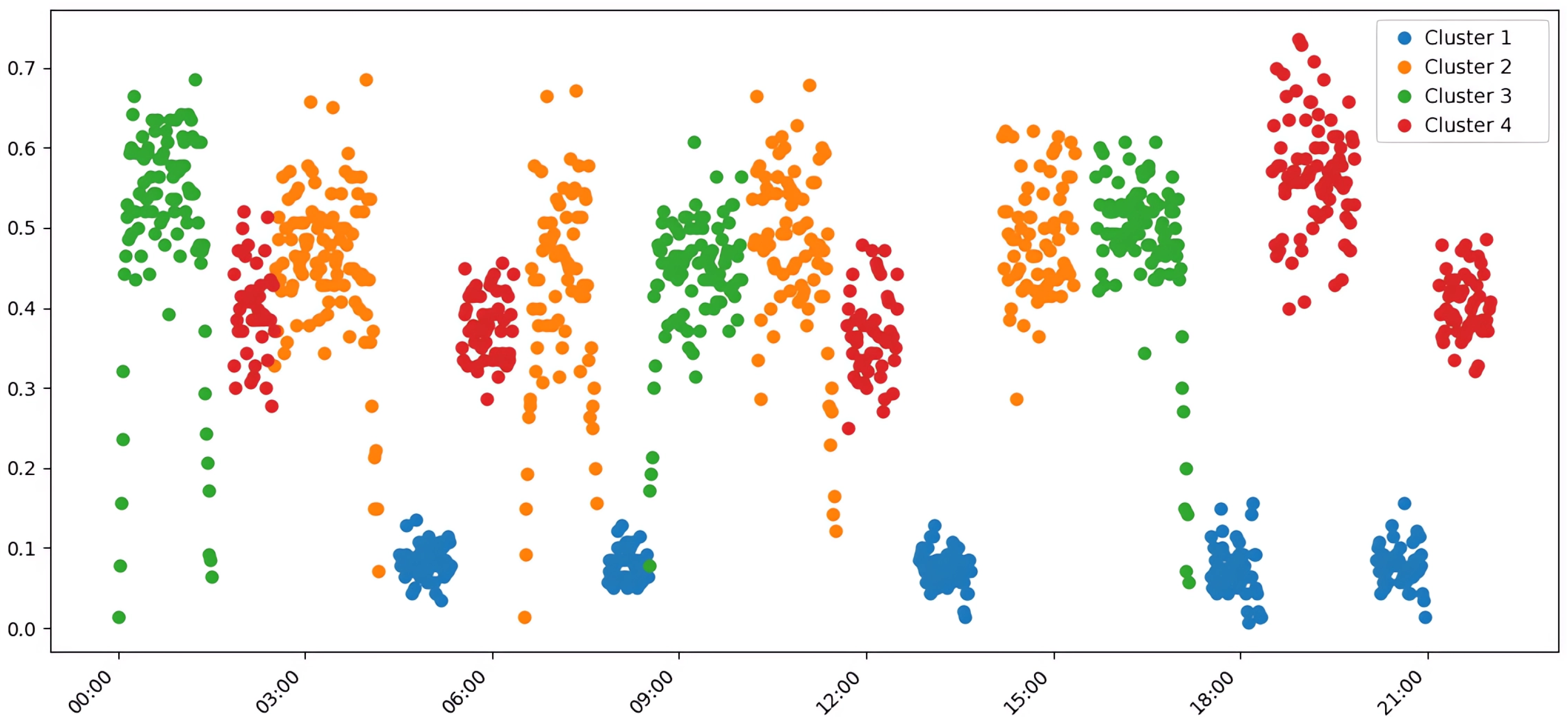
Clustering of aggregated average traffic data using HDBSCAN. The algorithm automatically identified eight distinct clusters, effectively separating the different simulated traffic modes and demonstrating a strong alignment with the ground-truth data structure. Each color represents a distinct traffic pattern.
Figure 4.
Clustering of aggregated average traffic data using k-means with K = 5. This approach produced compact, well-defined spherical clusters, which resulted in high internal validation scores. However, it also merged some distinct traffic scenarios (e.g., morning and evening peaks) into single groups, reducing its semantic accuracy.
Figure 5.
Clustering of aggregated average traffic data using k-means with K = 7. Increasing the cluster count resulted in the over-detailing and fragmentation of the data, where minor variations in traffic flow were incorrectly classified as separate patterns, thereby reducing the semantic clarity and interpretability of the clustering.
Figure 6.
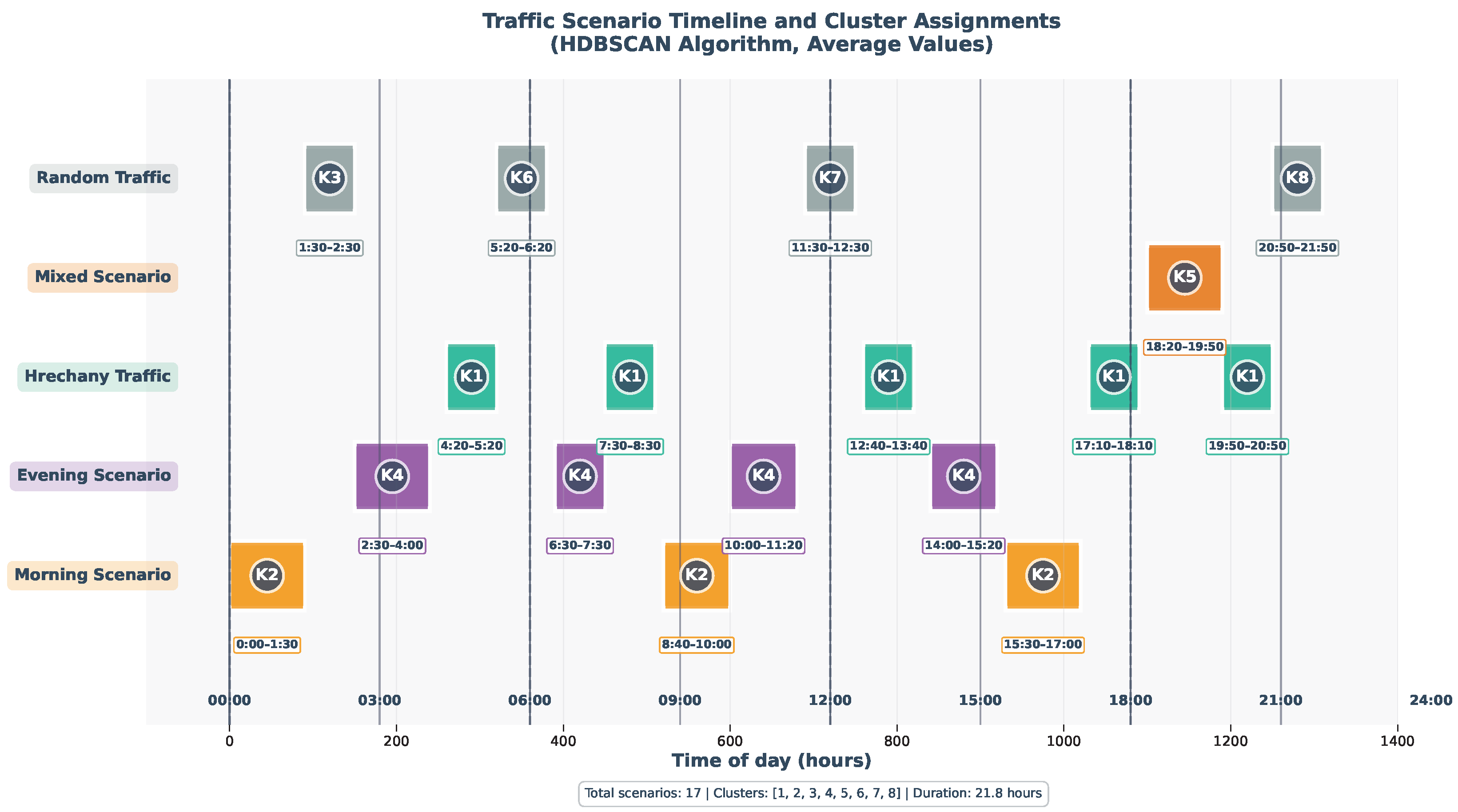
Temporal distribution of transport scenarios and their corresponding cluster assignments by the HDBSCAN algorithm on aggregated average data. Each colored block represents a specific cluster, showing a clear, non-overlapping, and chronologically consistent temporal sequence that aligns with the distinct traffic patterns throughout the simulated day.
Figure 7.
Distribution of experimental scenarios within the clusters identified by HDBSCAN on aggregated average data. (a) A bar chart detailing the number of scenarios per cluster, showing a balanced and meaningful distribution. (b) A pie chart illustrating the proportion of each scenario type in the experiment, highlighting the five primary traffic modes: Hrechany, Evening, Random, Morning, and Mixed.
Table 1.
Clustering performance on aggregated average traffic data. External and internal validation metrics are presented for HDBSCAN, k-means (K = 5), and k-means (K = 7). Higher values are better for V-measure, Rand Index, ARI, NMI, Fowlkes–Mallows, Silhouette, and Calinski–Harabasz scores; lower is better for the Davies–Bouldin Index.
| Approach | V-Measure | Rand Index | ARI | NMI | Fowlkes–Mallows | Silhouette | Calinski–Harabasz | Davies–Bouldin |
|---|
| HDBSCAN | 0.79 | 0.93 | 0.73 | 0.79 | 0.78 | 0.52 | 124.95 | 0.92 |
| k-means (K = 5) | 0.73 | 0.90 | 0.70 | 0.73 | 0.76 | 0.57 | 292.23 | 0.65 |
| k-means (K = 7) | 0.70 | 0.89 | 0.63 | 0.70 | 0.70 | 0.53 | 265.10 | 0.84 |
Table 2.
Clustering performance on high-dimensional combined traffic data. The table presents a full suite of validation metrics for HDBSCAN and k-means, illustrating the significant impact of increased data dimensionality on the performance of both algorithms.
Table 2.
Clustering performance on high-dimensional combined traffic data. The table presents a full suite of validation metrics for HDBSCAN and k-means, illustrating the significant impact of increased data dimensionality on the performance of both algorithms.
| Approach | V-Measure | Rand Index | ARI | NMI | Fowlkes–Mallows | Silhouette | Calinski–Harabasz | Davies–Bouldin |
|---|
| HDBSCAN | 0.64 | 0.88 | 0.61 | 0.64 | 0.68 | 0.26 | 42.83 | 1.49 |
| k-means (K = 5) | 0.67 | 0.87 | 0.62 | 0.67 | 0.71 | 0.23 | 34.79 | 1.59 |
| k-means (K = 7) | 0.66 | 0.88 | 0.59 | 0.66 | 0.67 | 0.19 | 26.84 | 2.14 |
Table 3.
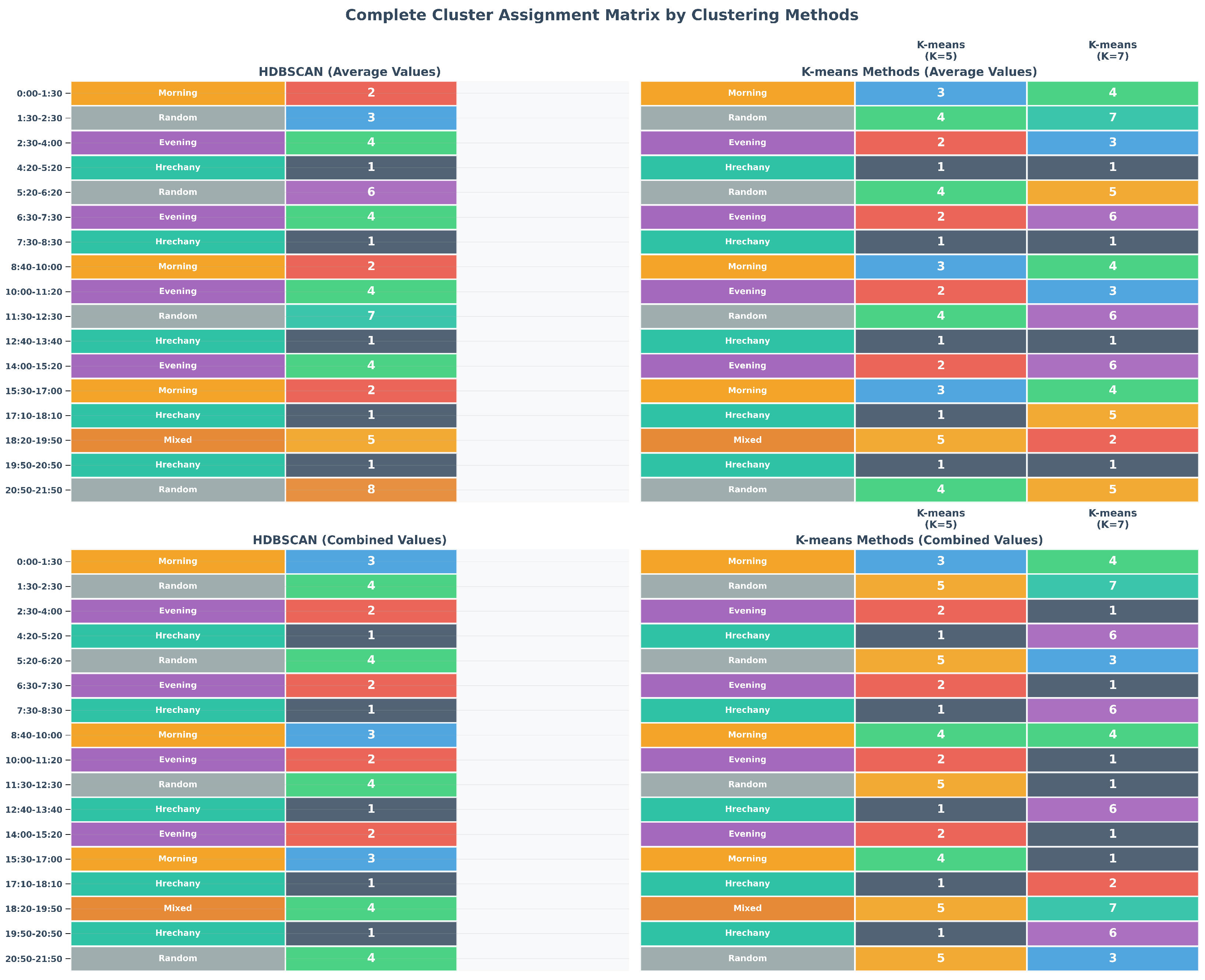
Cluster assignments for key transport scenarios on aggregated average data. The table shows the categorization of different time periods and specific, named scenarios by the HDBSCAN, k-means (K = 5), and k-means (K = 7) algorithms, providing insight into their semantic interpretation of the data.
| Time Period | Scenario Type | HDBSCAN | k-Means (K = 5) | k-Means (K = 7) |
|---|
| 00:00–01:30 | Morning | Cluster 2 | Cluster 3 | Cluster 4 |
| 01:30–02:30 | Random No. 1 | Cluster 3 | Cluster 4 | Cluster 7 |
| 02:30–04:00 | Evening | Cluster 4 | Cluster 2 | Cluster 3 |
| 04:20–05:20 | Hrechany | Cluster 1 | Cluster 1 | Cluster 1 |
| 05:20–06:20 | Random No. 2 | Cluster 6 | Cluster 4 | Cluster 5 |
| 06:30–07:30 | Evening (variation) | Cluster 4 | Cluster 2 | Cluster 6 and 3 |
| 07:30–08:30 | Hrechany (variation) | Cluster 1 | Cluster 1 | Cluster 1 |
Table 4.
Performance comparison between the standalone algorithms and the final cascade approach. The table showcases the significant improvements in both clustering structure quality (V-measure) and cluster compactness (Silhouette Score) achieved by the adaptive approach.
Table 4.
Performance comparison between the standalone algorithms and the final cascade approach. The table showcases the significant improvements in both clustering structure quality (V-measure) and cluster compactness (Silhouette Score) achieved by the adaptive approach.
| Criterion | HDBSCAN (Standalone) | k-Means (K = 5, Standalone) | Cascade Approach |
|---|
| Structure Quality (V-measure) | 0.79 | 0.73 | 0.79–0.82 (+0–4%) |
| Cluster Compactness | 0.52 | 0.57 | 0.57–0.59 (+10–14%) |
Table 5.
Scenario identification accuracy rates for the different clustering approaches. The table shows the percentage accuracy for identifying five distinct transport scenarios and the overall average accuracy for each algorithm.
Table 5.
Scenario identification accuracy rates for the different clustering approaches. The table shows the percentage accuracy for identifying five distinct transport scenarios and the overall average accuracy for each algorithm.
| Scenario Type | HDBSCAN (%) | k-Means (K = 5) (%) | k-Means (K = 7) (%) | Cascade Approach 1 (%) |
|---|
| Morning Peaks | 95 | 92 | 88 | 95–97 |
| Evening Peaks | 93 | 90 | 85 | 93–96 |
| Hrechany Scenario | 98 | 98 | 98 | 98 |
| Mixed Modes | 91 | 85 | 82 | 91–94 |
| Low-Active Periods | 87 | 83 | 79 | 87–90 |
| Average Accuracy | 92.8 | 89.6 | 86.4 | 92.8–95.0 |
Table 6.
Robustness of the clustering algorithms to the addition of noise, as measured by the ARI. The table shows the degradation in quality for each approach as the level of Gaussian noise is increased from 0% to 35%.
Table 6.
Robustness of the clustering algorithms to the addition of noise, as measured by the ARI. The table shows the degradation in quality for each approach as the level of Gaussian noise is increased from 0% to 35%.
| Noise Level | HDBSCAN | k-Means (K = 5) | k-Means (K = 7) | Cascade Approach 1 |
|---|
| 0% (basic) | 0.73 | 0.70 | 0.63 | 0.73 |
| 15% | 0.71 (−3%) | 0.64 (−8%) | 0.58 (−8%) | 0.71 (−3%) |
| 25% | 0.68 (−7%) | 0.60 (−15%) | 0.53 (−16%) | 0.68 (−7%) |
| 35% | 0.65 (−11%) | 0.55 (−21%) | 0.48 (−24%) | 0.65 (−11%) |
Table 7.
Temporal coherence analysis of the clustering results. The table compares the temporal consistency of the clusters generated by each approach, as measured by a coherence coefficient and the number of temporal intersections (overlaps).
Table 7.
Temporal coherence analysis of the clustering results. The table compares the temporal consistency of the clusters generated by each approach, as measured by a coherence coefficient and the number of temporal intersections (overlaps).
| Approach | Coherence Coefficient | Intersections in Time |
|---|
| HDBSCAN | 0.94 | 0 |
| k-means (K = 5) | 0.89 | 2 |
| k-means (K = 7) | 0.85 | 5 |
| Our Approach | 0.94 | 0 |
Table 8.
Statistical significance of performance differences, as determined by the Wilcoxon signed-rank test. The table shows the W-statistic and the corresponding p-value for key comparisons, confirming the statistical significance of the observed advantages.
Table 8.
Statistical significance of performance differences, as determined by the Wilcoxon signed-rank test. The table shows the W-statistic and the corresponding p-value for key comparisons, confirming the statistical significance of the observed advantages.
| Comparison | W-Statistic | p-Value |
|---|
| HDBSCAN vs. k-means (K = 5) on external metrics | 78 | 0.008 |
| HDBSCAN vs. k-means (K = 7) on external metrics | 85 | 0.003 |
| Aggregated Average Data vs. High-Dimensional Combined Values | 92 | 0.002 |


