Article

Deep Reinforcement Learning Approach for Traffic Light Control and Transit Priority

Department of Civil, Environmental and Constructional Engineering, Sapienza University of Rome, Via Eudossiana, 18, 00184 Rome, Italy
*
Author to whom correspondence should be addressed.
Future Transp. 2025, 5(4), 137; https://doi.org/10.3390/futuretransp5040137
Submission received: 8 October 2024 / Revised: 20 June 2025 / Accepted: 15 July 2025 / Published: 4 October 2025

Abstract

This study investigates the use of deep reinforcement learning techniques to improve traffic signal control systems through the integration of deep learning and reinforcement learning approaches. The purpose of a deep reinforcement learning architecture is to provide adaptive control via a reinforcement learning interface and deep learning for the representation of traffic queues with regards to signal timings. This has driven recent research, which has reported success in the use of such dynamic approaches. To further explore this success, we apply a deep reinforcement learning algorithm over a grid of 21 interconnected traffic signalized intersections and monitor its effectiveness. Unlike previous research, which often examined isolated or idealized scenarios, our model is applied to the real-world traffic network of Via “Prenestina” in eastern Rome. We utilize the Simulation of Urban MObility (SUMO) platform to simulate and test the model. This study has two main objectives: ensure the algorithm’s correct implementation in a real traffic network and assess its impact on public transportation, incorporating an additional priority reward for public transport. The simulation results confirm the model’s effectiveness in optimizing traffic signals and reducing delays for public transport.

1. Introduction

Traffic demand slows down the speed of the traffic stream due to interactions among vehicles, which results in congestion. Massive queues build up with consequent high levels of fuel consumption and pollutant emissions, waiting time increases with delays, and road users often experience dissatisfaction when they encounter delays at their destinations as a result of congestion. Additionally, not only private vehicles but also public transport vehicles (buses and trams), which travel through the same links and junctions of the city multiple times a day, are involved in road congestion. This results in bus or tram delays, vehicle bouncing, long queues at bus stations, increased waiting times, and an overall decline in reliability and satisfaction [1]. According to The Economist, traffic congestion in the European Union costs approximately 1% of GDP [2].
To manage this issue, traffic signal control (TSC) strategies are classified according to their adaptability and level of hierarchy. Adaptability is foundational, as it defines how a control approach can respond to varying traffic demands. TSC strategies generally include fixed-time or dynamic approaches. Fixed-time strategies calculate the cycle length offline based on historical demand and turn patterns, which makes them effective in the case of planned demand levels but less adaptable to real-time fluctuations. As traffic conditions change, fixed timing can quickly become inefficient [3].
In the context of urban traffic, traditional TSC systems such as Fixed-Time [4] and adaptive systems like SOTL [5] and Max-Pressure [6] are widely used but have scalability limitations, especially as traffic volumes increase. These systems are often built upon a set of pre-made assumptions about traffic, which may not reflect real-world variability and can cause reduced effectiveness under fluctuating conditions [3]. Dynamic timing, on the other hand, allows for the adjustment of cycle elements—such as green, red, and yellow times—based on current demand, which makes it more effective in adapting to variable traffic levels [7]. The hierarchical control level of TSC strategies determines whether control is managed locally or coordinated across multiple intersections. In local control, only data from the immediate intersection are considered, which can lead to network inefficiencies, such as spillbacks or uncoordinated signal plans that increase vehicle stops. Coordinated control, on the other hand, integrates data from neighboring intersections, potentially improving network performance [8]. Combinations of these strategies, such as local dynamic and local fixed-time control, are also explored in practice.
Given the need to handle increasingly complex traffic demands, recent research has turned to reinforcement learning (RL) to dynamically optimize TSC in real time. RL provides a framework where an agent learns to perform actions—such as adjusting traffic signals—by receiving immediate feedback (rewards) from its environment, which is represented by the current traffic state. A key challenge in applying RL to TSC is designing appropriate state and reward structures to ensure that the agent develops an effective action-selection policy without being constrained by assumptions that are better suited to simulations than real-world scenarios [9]. Furthermore, a common issue in RL-based TSC is how to achieve optimal action-selection policies by aligning state and reward definitions realistically, thereby enhancing convergence to optimal solutions [10].
In recent years, combining reinforcement learning with deep learning (DRL) has enhanced TSC systems further (Figure 1). DRL-based solutions, particularly deep Q-networks (DQNs), capitalize on the ability of deep learning to recognize complex patterns, enabling more intelligent intersections and allowing TSC to handle variable traffic densities and dynamic flows with greater flexibility [11,12,13]. This integration of deep learning enables better performance than traditional TSC techniques, which are limited by their fixed assumptions about traffic [14].
Due to two major difficulties, traditional reinforcement learning is challenging to implement: (1) how to describe the environment and (2) how to model the relationship between the environment and the decision. Recent studies have used deep reinforcement learning approaches, such as deep Q-learning (DQN), for traffic light management problems to overcome these two issues [2].
More recent advancements include approaches such as spatiotemporal graph attention networks and multi-agent frameworks, which allow for better coordination across intersections and capture more complex spatial dependencies [15,16]. However, these methods often rely on synthetic networks or simplified assumptions about vehicle or passenger flow.
Other emerging directions include federated reinforcement learning, where decentralized training is used to preserve data privacy while allowing control policies to adapt across distributed intersections [17]. While promising, such models still lack validation in operational environments with real-world public transit demand.
Recent studies have also explored multimodal signal control strategies that integrate transit priority using multi-agent reinforcement learning, including decentralized frameworks for bus holding and adaptive green extension [18]. Despite the innovations, these models often operate in idealized settings and do not fully evaluate their impact on both private vehicle and public transport performance under empirical demand.
Building on this foundation, our approach introduces several key contributions to further advance this field.
  • Traffic signal priority for public transport. The model uses a CNN to process visual or spatial input to extract key features such as type of vehicle (public or private). Priority action might include allowing for green signals when public transport is detected. However, the reward signal is balanced in a way to prevent excessive congestion for non-priority vehicles. The CNN continuously extracts real-time features from traffic data. Based on these features, the DRL agent determines the most effective signal phase to prioritize public transport while maintaining overall traffic efficiency. The advantage of this approach is that the public transport efficiency improves without significantly disturbing general traffic.
  • Experience with real-world network and traffic data. With advancements in technology, many major cities are now equipped with monitoring systems like surveillance cameras. However, most existing studies rely on experimental data to test their algorithms. Among the works that utilize real-world data, calibration and validation are, to the best of the authors’ knowledge, often not addressed or presented. In contrast, our study utilizes real-world data provided by the Agency of Mobility of Rome, collected over the course of one month. Furthermore, the network corresponding to these data represents a major corridor with 21 sequential traffic lights, unlike other studies that focus on idealized intersections.
  • Complexity of intersection geometrical configuration and traffic light phases in a real-world scenario. The intersections in this study consist of multiple complex phases, including four-phase traffic lights with delayed turning movements, which present significant challenges for the DRL agent in decision making. This complexity is further heightened when considering multiple intersections, as the timing of left-turn movements for the eastbound approach and right-turn movements for the westbound approach must be coordinated with adjacent intersections to prevent spillback. A traffic management action that alleviates congestion at one intersection may inadvertently cause delays at upstream intersections. Therefore, turning movements are explicitly incorporated into the state representation to ensure that the agent can account for these interdependencies and optimize traffic flow across the network.

2. Literature Review

Reinforcement learning (RL) is a class of learning problems which involves the optimization of sequential decisions by agents who interact with their surroundings and learn from such interactions. In other words, the core aim of RL is to learn a policy such that the current state of the environment is a key reference of the action that the agent will undertake at that point in time. After some time, RL was somewhat stagnant with respect to its prospects of use, but things changed with the advent of function approximators, notably the use of neural networks for Deep RL in the 2010s [14]. The application of RL and DL in tandem has contributed to remarkable progress with respect to the needs in various areas, including video games [19], energy efficiency [20], and VANET security [21,22]. Of these fields, transportation has been the area where Deep RL is expected to make a difference. It has been reported that recent studies have sought to enhance traditional traffic control signal systems by Deep RL methods, which are viewed as the new traffic control system [13,23,24,25]. This indeed makes it a novel approach to the problems posed in relation to transportation systems.

2.1. State Representation

In the literature on DRL-based traffic signal control (TSC), the state reflects the information that the agent perceives from traffic intersections to determine the appropriate action at each time step. Defining the state is crucial, since the agent’s behavior is heavily influenced by the information it receives from the environment. For example, [13] introduced the concept of discrete traffic state encoding (DTSE), which has become a widely adopted state definition. In DTSE, each lane, with length l, is divided into cells of length c. Each cell contains information relevant to the state of a vehicle approaching the intersection. DTSE is formally composed of three vectors: (1) vehicle presence or absence, (2) vehicle speed, and (3) the current traffic signal phase. These vectors are combined into an image-like array that can be processed using Convolutional Neural Networks (CNNs) [26]. Beyond DTSE, other researchers [27] have explored using virtual snapshot images of the intersection, extracted from simulators. These images are divided into grids, with each cell capturing information such as vehicle position and speed. Alternatively, some studies [28] have opted for a feature-based value vector to represent the intersection state. In this approach, each vector element stores specific lane-related data, such as vehicle count, queue length, and updated waiting times. This representation is more practical and easier to implement at intersections equipped with sensors and induction loops compared with more complex state definitions. A simpler state representation, as suggested by Zheng et al. [28], can sometimes yield better results. Their work demonstrated the effectiveness of a concise state and reward design, using the number of vehicles and queue length for state and reward definitions, respectively. Despite the promising outcomes in their study, further refinement and enhancement of state and reward definitions are necessary, as explored in this work.

2.2. Reward Function

The reward represents the feedback that the agent receives from the environment after performing an action, serving to distinguish favorable and unfavorable events for the agent [29]. Although it is a scalar value, the way the reward is defined plays a pivotal role in shaping the learning process of the reinforcement learning agent. In the context of optimizing traffic control with RL, the typical global objective for the TSC agent is to reduce the average travel time of vehicles from their origin to their destination [13]. However, because the average travel time is a long-term goal and the agent only receives feedback at the end of an episode, it cannot be directly used as a reward function. Instead, alternative reward definitions are needed to approximate the primary objective. Several reward formulations have been proposed, including the change in total waiting time, queue length, and cumulative vehicle delay [13,26,28,30]. Wei et al. [2] introduced a more complex reward definition, using a weighted sum of multiple reward components. More recently, Zheng et al. [28] compared various reward formulations and found that defining the reward based on queue length produced better results than other approaches, including the weighted sum method. Additionally, Wei et al. [31], leveraging traditional algorithms, employed “pressure” as a reward formula, which demonstrated improved performance over earlier methods.

2.3. Action Space Definition

For optimal behavior, an RL agent should select the appropriate action for the observed state that maximizes the discounted cumulative reward. The definition of the action space depends on the specific application. In RL applied to traffic signal control, the agent’s action influences the traffic signal phase in different ways. Typically, action spaces are categorized into three types.
The first type is a binary action space, where the agent decides whether to extend the current phase or switch to the next phase in a predefined sequence [2,28]. The second type involves a larger action space, allowing the agent to choose from four or eight phases at a four-leg intersection, with no fixed sequence required. These two discrete action spaces are the most commonly used in the literature [13,31,32]. The third type, used in some studies, employs a continuous action space in which the agent determines the optimal phase duration splits within a fixed cycle length [33].

2.4. Markov Decision Process

The primary formulation for applying RL to traffic signal control (TSC) involves the use of Markov decision processes (MDPs). This problem formulation can be formally represented as a tuple (S, A, T, R, γ). Within an MDP, a single controller agent interacts with an environment, usually at a single intersection, over a series of time steps t ∈ {1. T}. At each time step, the agent makes decisions based on the current state of the system. The controller receives a representation of the current state of the intersection, denoted by stS, where S represents the set of all possible states. To simplify the problem, st is typically an abstracted numerical representation of the intersection. According to a review by [34], common elements included in intersection-level state representations are (1) the queue length, (2) the current phase, (3) the total number of vehicles, (4) the positions of vehicles, and (5) the speeds of vehicles. Based on the current state st, the controller selects an action atA to perform, where A represents the set of all possible actions (assumed to be the same for each state). In most works, agents choose the next phase and its duration as the action. In other works, the action space is based on cycles, allowing for variations in the phase split and sequence within fixed-length cycles or changes in the cycle length. The action performed by the controller immediately influences the intersection, leading to a transition to the next state with a certain probability. This transition represents the immediate impact of the signaling decision. Given the current state st and action at, each possible next state st + 1 ∈ S occurs with a probability denoted by T (st, at, st + 1), which represents the probability of transitioning to st + 1 given st and at. It satisfies the condition that the sum of probabilities over all possible next states st + 1 equals 1, for all st and at. Upon performing the action, the controller receives a numerical reward t (st, at, st + 1) ∈ R, which quantifies the effectiveness of the signaling decision. In the context of traffic signal control (TSC), this reward can be determined based on the updated state. As mentioned in [34], some of the approaches utilize queue lengths, while a minor percentage consider vehicle counts. Alternatively, the reward can be derived from vehicle-specific quality metrics. For instance, some methods employ vehicle delays, measured as an increase in travel time, waiting time of vehicles, and intersection throughput. By utilizing these rewards, the agent learns to assess the quality of signaling decisions across different intersection states.
The objective of the controller is to acquire a policy π: SA that determines the appropriate action to perform given the current state: at = π(st). The goal is to find an optimal policy that maximizes the cumulative rewards, represented by the sum of rewards over time t = 1 T r t .

2.5. Bellman Equation

Learning an ideal strategy to maximize the cumulative expected rewards from the current state is the aim of reinforcement learning. However, this is a sequential problem, and the agent cannot simply select actions that maximize the immediate estimated rewards at each time step [35]. This is because the agent’s decisions can impact future time steps, influencing the state at those points. For example, clearing one intersection at time step t may result in congestion at another intersection in the subsequent time step t + 1 . To account for this, the Q-value function Q (s, a) takes into consideration the expected rewards of future time steps while assigning a decreasing weight to them, reflecting the long-term implications of the agent’s actions.
         Q π s , a = E r t + γ r t + 1 + γ 2 r t + 2 + S t = s , a t = a , π = E   k = 0 γ k r t + k | S t = s , a t = a , π
The discount factor, denoted by γ and ranging between 0 and 1 (in the range [0,1)), is incorporated in the Q-value function. Essentially, the Q-value represents the value associated with making a signaling decision in a specific state, considering that the best decision is consistently made in the future. In other words, the Q-value takes into account the notion that the value of a decision is influenced by the potential future decisions and their associated rewards, with the discount factor determining the weight assigned to future rewards. Yet, the nearest rewards are more valuable than the rewards in the further future. The best course of action is simply to take the biggest overall reward if the agent is aware of the optimal Q-values for the subsequent states. Considering the succeeding states’ optimal Q-values, the optimal Q (s, a) is computed. The Bellman optimality equation can be used to compute Q π * (s, a) [12].
Q π * s , a = E s r t + γ m a x Q π * ( s t + 1 , a t + 1 ) s , a

2.6. Deep Neural Networks

Recent works [2,36] suggest integrating deep learning techniques with reinforcement learning (RL), a combination commonly known as deep reinforcement learning (DRL). The key goal of this fusion is to approximate the policy function using deep neural network (DNN) models. Earlier research [37] utilized deep Stacked-AutoEncoders (DeepSAE) as the DNN structure for DRL, whereas more recent approaches employ stacked convolutional layers (Conv) paired with a flatten layer and multiple Fully Connected (FC) layers. The flatten layer transforms the two-dimensional feature maps generated by the convolution layers into a one-dimensional vector, which is then fed into the FC layers. These DNN models, which include convolution layers designed to replicate the biological convolution processes in the human visual cortex, are commonly referred to as Convolutional Neural Networks (CNNs) [38]. By adding more convolution layers, CNNs can further extract features from previously derived features through a process of sub-sampling, converting lower-level features into higher-level ones, thus potentially improving overall model performance [13]. The FC layers of the CNN serve the purpose of classifying the structural condition and forecasting the chances of executing any of the available actions depending on the input given to the CNN. As opposed to what happens in image classification, the DRL uses the CNN model without the pooling layers, since it is very important in traffic control to know the exact places of traffic variations in the image-like inputs.

2.7. Transit Signal Priority Using DLR

Using RL algorithms is also regarded as the way in which a more satisfactory Transit Signal Priority (TSP) can be attained. In this approach, instead of studying many conditions and algorithms, there is the creation of an interaction structure wherein the agent and the environment engage. The agent observes the condition around the agent, which incorporates trams, buses, personal vehicles, and even the timing of signals. The agent acts in response to the learning to opt for actions that are most likely to produce a reward. After the agent executes these activities, the environment carries out the actions, changes the lights, and gives the agent the next status and instant rewards. Therefore, this model free-RL technique accommodates the changing state of traffic without the use of optimizing models. The first attempt at the use of RL in TSP was Adaptative TSP for a single intersection along the King Streetcar route using a tabular Q-learning algorithm to reduce deviations from the desired headways [39]. Yet, in the case study, which deals with one streetcar route, it is clear that the intricacies of cross bus routes traffic at junctions is understudied. Following this, DRL approaches such as deep Q-network (DQN) [39] and proximal policy optimization with model-based acceleration (PPOMA) [40] were used to propose TSP approaches in the frame of state space with high dimensionality.

3. Problem Definition

This research study focuses on the control of traffic lights at intersections. Intersections typically have three signals, green, yellow, and red, which guide the flow of vehicles from different directions. In some cases, a single traffic light may not be sufficient to manage all the vehicles, and multiple traffic lights must work together at a multi-direction intersection. Each traffic light changes its status to guide vehicles from non-conflicting directions at a given time. A setting of the traffic light is defined as a phase. When light changes from green to red there is a (4 s) yellow light. Phases cycle in a fixed sequence to facilitate vehicle movement through the intersection, forming a complete cycle. Although the sequence of phases remains fixed, the duration of each phase can be adaptively adjusted based on the current traffic conditions. In our problem, we aim to dynamically optimize the duration of each phase to minimize delay and enhance intersection efficiency in response to varying traffic situations. By leveraging historical experiences, we learn to modify the duration of each phase strategically. If a particular phase has a higher number of vehicles or a public transit vehicle (tram), its duration is extended. Additionally, to prioritize trams over private vehicles, we have considered an additional reward for them. Our approach involves a self-updating network that continuously receives states and rewards from the environment. The traffic light processes these data to determine the state of road traffic and the associated reward, a common assumption in previous studies [13,41]. Based on the current state and reward, the traffic light selects an action by using a deep neural network.

4. Framework

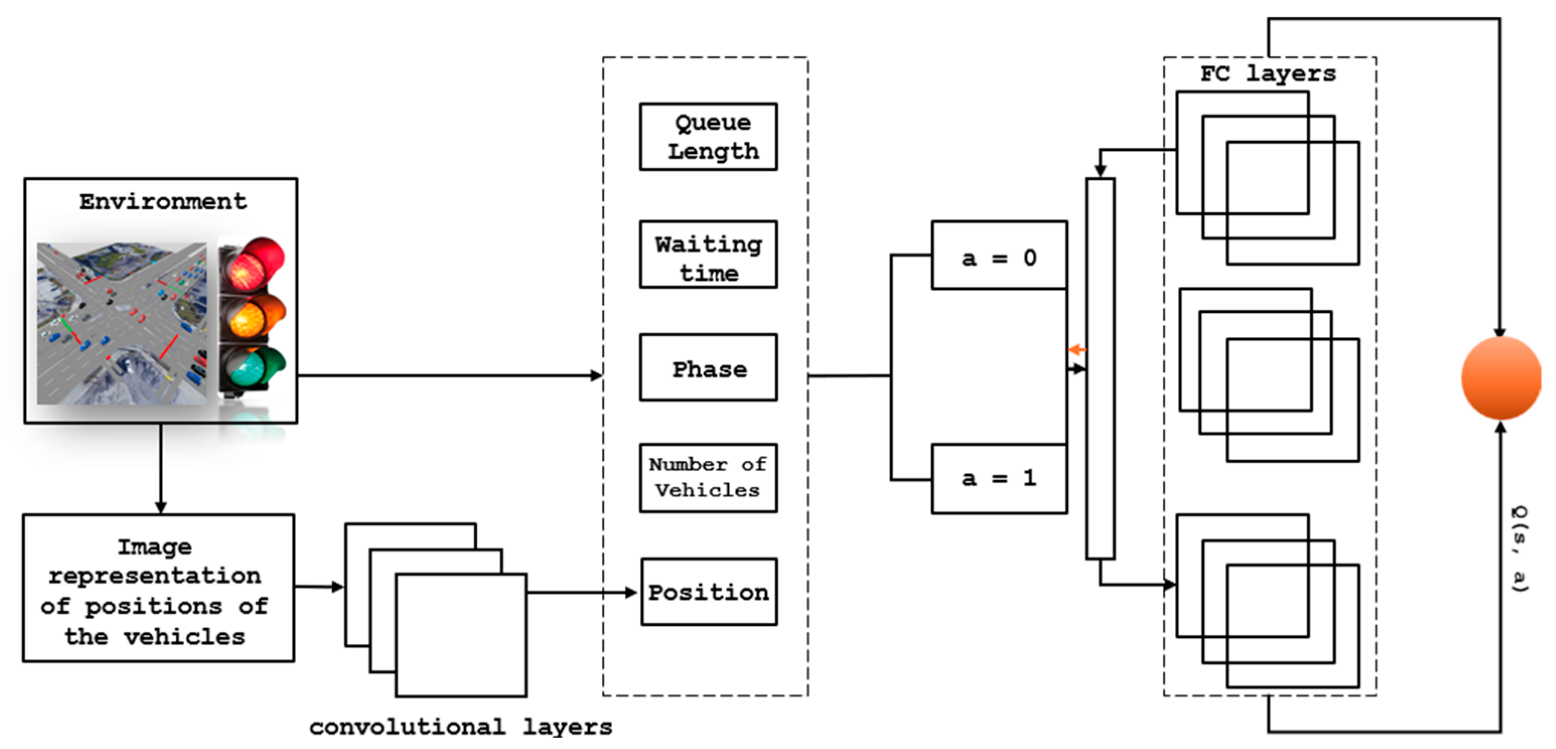
We have adopted a common model framework from previous studies that consists of two components: an online part and an offline part [2]. Figure 2 illustrates the model framework.
  • Offline Stage: In the offline stage, a fixed timetable for the traffic lights is set. Data samples are collected by allowing traffic to flow through the system based on the fixed timetable. During this stage, the model logs the collected data samples.
  • Training: The collected data samples are then used for training the model. The training process involves using the logged data samples to update the model’s parameters.
  • Online Stage: After the model is trained, it proceeds to the online stage. In a regular time interval (Δt), the traffic light agent observes the current state (s) of its environment. The agent then performs an action (a) based on the observed state, which will determine whether it changes to another light phase or not. The action-selection strategy follows the ε-greedy strategy by combining exploration (doing random actions with probability ε) and exploitation (selecting the action with the maximum expected reward).
  • Observing Rewards: After performing the action, the agent observes the environment and receives a reward (r) based on how much the action has improved the traffic conditions. The reward is a measure of the quality of the agent’s decision and indicates the impact of the action on traffic flow.
  • Memory and Network Updates: The tuple (s, a, r) consisting of the observed state, performed action, and received reward is stored in a memory buffer. After a certain number of timestamps or a specific condition is met, the agent updates the network by using the logged data in the memory buffer.

4.1. Agent Design and Reward Calculations

As mentioned earlier, reinforcement learning is a machine learning algorithm that is different from supervised and unsupervised learning. Its objective is to act in a way that will ultimately maximize the final reward. An agent, known as the action executor, performs an action in reinforcement learning, and the environment responds by returning a numerical reward based on the action and the current state.
To define reinforcement learning we can use a tuple of three (S, A, R):
  • S: It represents our state, which includes the queue length on the lane, the number of vehicles, and the average waiting time. The state also includes the position of the vehicle, as well as the current phase and the next phase.
  • A: Action is defined as changing the light to the next phase (a = 1) or keeping the current phase (a = 0).
  • R: Two different rewards were calculated for the scenario without TSP (hereafter scenario 1) and the scenario with TSP (hereafter scenario 2):
Scenario 1: Reward is a weighted sum of the parameters below:
  • The sum of the queue length: The queue length ( q l ) for a specific lane is determined by counting the total number of vehicles in the queue plus the minimum gap between them.
  • The sum of time loss for all vehicles due to driving below the ideal speed (the ideal speed includes the individual speed factor; slowdowns due to intersection).
  • The number of traffic light switches involves counting the occurrences when the current phase of the traffic lights is either kept unchanged (C = 0) or changed to a different phase (C = 1).
  • The sum of waiting time is the sum of the waiting time of all the vehicles across all lanes approaching the intersection ( W l ).
  • The total number of vehicles that have passed the intersection during the time interval τ after the last action (n).
R e w a r d   1 = ω 1 l   ϵ   L q l   + ω 2 l   ϵ   L D l   + ω 3 C + ω 4 l   ϵ   L W l   + ω 6 n
Scenario 2: Reward is a weighted sum of the parameters below:
  • The sum of the queue length: The queue length ( q l ) for a specific lane.
  • The sum of the time loss for private vehicles.
  • The sum of the time loss for public transport ( D p ).
  • The number of traffic light switches involves counting the occurrences when the current phase of the traffic lights is either kept unchanged (C = 0) or changed to a different phase (C = 1).
  • The sum of waiting time is the sum of the waiting time of private vehicles across all lanes approaching the intersection ( W l   ).
  • The sum of the waiting time of public transport vehicles approaching the intersection W p .
  • The total number of vehicles that have passed the intersection during the time interval τ after the last action (n).
R e w a r d 2 = ω 1 l   ϵ   L q l   + ω 2 l   ϵ   L D l   + ω 3 l   ϵ   L D p + ω 4 C + ω 5 l   ϵ   L W l   + ω 6 l   ϵ   L W p   + ω 7 n

4.2. Network Structure

From the observations of the traffic situation, the current state is taken and fed into two convolutional layers. The four specifically mined features, queue length L, average waiting time W, phase P, and total number of vehicles V, are added to the output of these layers. In order to understand the mapping from traffic circumstances to potential rewards, the concatenated characteristics are subsequently fed into fully linked layers. Then, we develop a unique learning approach for mapping rewards to the value of decision making for each phase Q (s, a).
These distinct processes are chosen via a gate controlled by the phase. As illustrated in Figure 3, when phase C = 0, the top branch is activated, whereas when phase C = 1, the bottom branch is activated. This will distinguish the decision process for different phases, prevent their decisions from favoring specific actions, and improve the network’s fitting ability.

4.3. Parameter Setting

The discount factor is typically advised to be set to 0.9, and the learning rate is suggested to be 1 × 10⁻³ [3,41,42]. Table 1 describes the hyperparameters used in the training.

5. Experimental Environment

5.1. Microsimulation

In TSC, it is not practical to try and recreate the transition probabilities for TSC. This has led to the practice of using traffic simulators with the aim of creating training experiences. Apart from the use of RL approaches in simulations for TSC, the non-RL approaches in TSC have greatly depended on simulations which lead to the creation of many commercial and even free simulators which can work with RL [3]. Traffic simulators are primarily grouped into three types according to the degree of sophistication. The most advanced simulation is provided by microscopic simulators that follow one vehicle at a time while simulating movements such as acceleration, deceleration, or the changing of lanes. Such behavior follows the so-called car-following models, where a vehicle shows a time-dependent profile of acceleration apparently consisting of its own speed and the speeds of other vehicles. In contrast to these, there are macroscopic simulators that do not consider individual vehicles but rather flows of vehicles and time series describing the volume, speed, and density of flows at various points of the road network. As the name suggests, mesoscopic simulators can bridge the gap between the two extremes by either describing individual vehicles as fluid or platooning some vehicles. A study of traffic models such as fluidic, kinetic, and cell transmission in conjunction with computer simulations is provided in [43]. Among the traffic simulators used for training RL agents in TSC, the most common simulator (as reported in [34]) is SUMO.

5.2. Simulation of Urban Mobility (SUMO)

The assessment was conducted in SUMO, a platform that provides detailed, real-time traffic simulation with the versatility to model different signal plans, road configurations, and types of road users [44]. Python APIs (Python 3.6, SUMO TraCI, Keras 2.2.0, Tensor-Flow 1.9.0) are employed to implement the DQN algorithm, enabling real-time interaction with SUMO. SUMO’s main capabilities include building road networks, creating traffic demands, and gathering a range of traffic performance metrics. To execute a SUMO simulation, two main files are set up as follows:
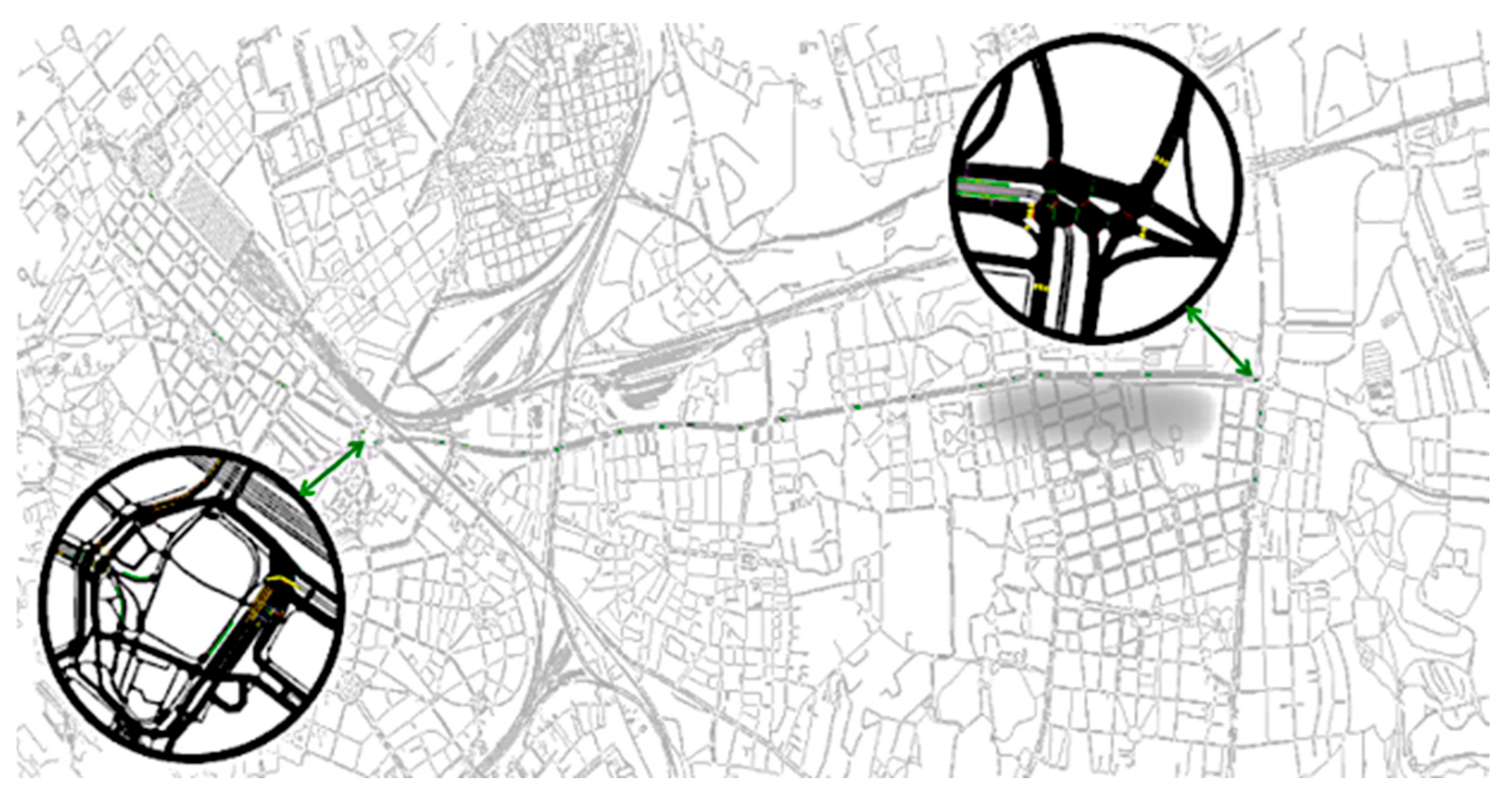
  • Road network file (net.xml): This file is responsible for creating the road network and configuring specific road characteristics (Figure 4).
  • Traffic route file (rou.xml): In this file, traffic requirements are input, and traffic scenarios are generated accordingly.
Additionally, there are other files, such as vehicle description files and detector description files, that can be included to enhance the simulation.
SUMO allows us to create a vast number of various measurements, which are automatically reported in XML files. The following are some of the available outputs:
  • Queue output: Calculation of the actual queue in front of a junction based on lanes.
  • Trip-info output (Trip information): Aggregated data on each vehicle’s trip (departure time, arrival time, duration, and route length)
  • Emission output: All vehicle emission values for each simulation step

5.3. Simulation Characteristics

The simulation considered four types of vehicles: passenger cars, city buses, motorcycles (converted into passenger cars), and trams. The count of motorcycles was converted into passenger cars based on the traffic norms of HCM (each two motorcycles were considered equivalent to one passenger car for simplicity in calibration).
The vehicle parameters are as shown in Table 2.
These parameters were derived from real-world traffic data and validated through calibration against observed traffic flows. The traffic flow followed a Poisson distribution, ensuring realistic vehicle arrivals at intersections. Following the warm-up period, the system was allowed to stabilize to achieve a steady state. Metrics such as average delay, throughput, and queue lengths were monitored to confirm steady-state conditions.
The emission model was based on HBEFA3/PC_G_EU4, reflecting real-world emissions standards. Specific emission factors for passenger cars, city buses, and trams were applied.

6. Study Area

The study area is the network corresponding to Via Prenestina (Figure 5), starting from the intersection of Via Palmiro Togliatti and Piazza Maggiore in the east part of Rome, in district V. The length of the corridor is 5100 m, with 21 signalized intersections in total, where 8 are two-phase, 6 are three-phase, and 7 are four-phase. Via Prenestina includes carriageways of two or three lanes for each direction, and it is characterized by the presence of the exclusive tram line in both directions, on which tram lines 5, 14, and 19 pass. The number of stops corresponding to these lines is 16 per direction. Via Prenestina was selected as the study area for this paper since, firstly, it has severe congestion and intersection delays and, secondly, it has a complex geometry of intersections.

7. Data Collection

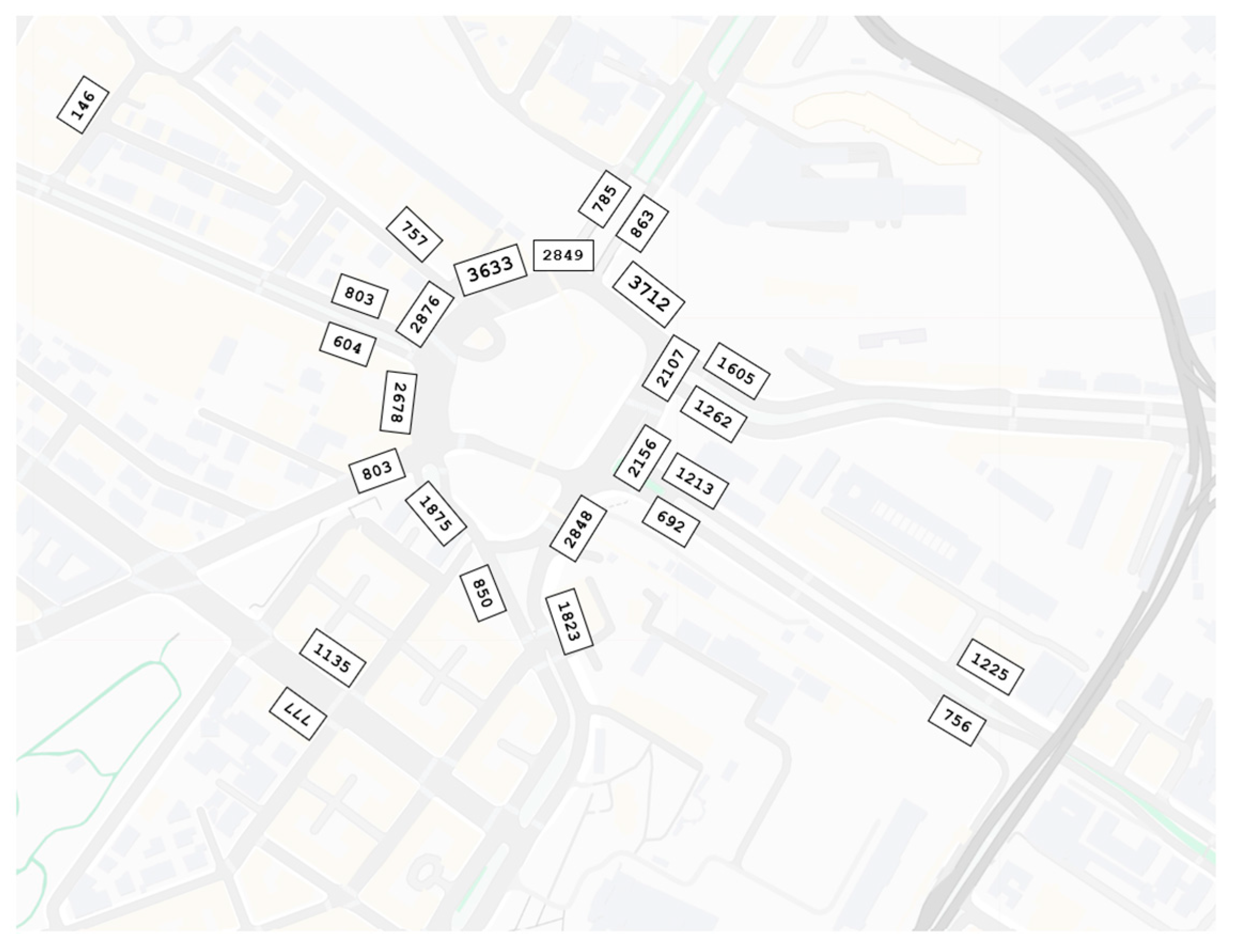
The two types of surveys that make up a traffic count survey are the counts of traffic on particular major corridors and the counts of traffic at particular intersections and public spaces. The primary goals of the traffic count survey are to measure current traffic volume on important thoroughfares, assess current traffic conditions, calibrate current OD matrices, and measure vehicle turning movements at significant intersections and squares. Figure 6, the traffic count of the major corridor, presents the flow volume at Porta Maggiore on both major and minor corridors. ATAC (Azienda Tramvie e Autobus del Comune di Roma) made the traffic counts available for each signalized intersection. The surveys were taken at three distinct times of day: morning rush hour (7:30–9:30), lunchtime (12:30–14:30), and evening rush hour (17:30–19:30). For each vehicle type and each allowed maneuver, data were collected. Because not all the junctions were monitored, flow balancing was performed for those that were not. ATAC has always produced timing diagrams of the current state of all traffic lights in the analyzed network. In addition, information on the route and frequency of tram lines 5, 14, and 19 was obtained from the ATAC website.

8. Calibration

Calibration is the fundamental process of adjusting specific model parameters so that the model can accurately replicate regional traffic performance measures and driver behavior.
To start with, one thing we do during the calibration process is identify the dyed points where queues remain for 15 min or more before dissipating. We combine all lanes and then determine the flow rate in those areas, which we convert to an equivalent hourly flow rate. Moreover, we consider the saturation flow rate per hour per lane for signalized junctions and study approach legs that experience queues of at least 10 vehicles per lane most commonly. It is worth noting that microsimulation models do not produce “capacity” as their output; instead, they give vehicle throughput numbers to particular locations. To mimic the maximum flow rate through bottlenecks, changes are made in input demand by creating a queue of vehicles upstream of target sections as necessary. When this happens, if the model does not initially show congestion at these bottlenecks like what has been observed in the field, we temporarily increase the coded demands so as to create congestion there. Once the capacity calibration is completed, these temporary increases should be removed before proceeding to the route choice calibration stage. For signalized junctions, the coded demand is adjusted as needed to ensure that at least 10 vehicles experience the required wait at the beginning of the green phase. We install detectors at the stop line in the model to monitor the discharge headways (per lane) of the first 10 vehicles crossing the detector. The per lane headways for each lane are then averaged, and the result is converted into a flow rate per lane per hour. Furthermore, during the calibration process, we consider various factors specific to signalized intersections, such as start-up lost time, queue discharge headway, and gap acceptance for unprotected left turns.

9. Validation

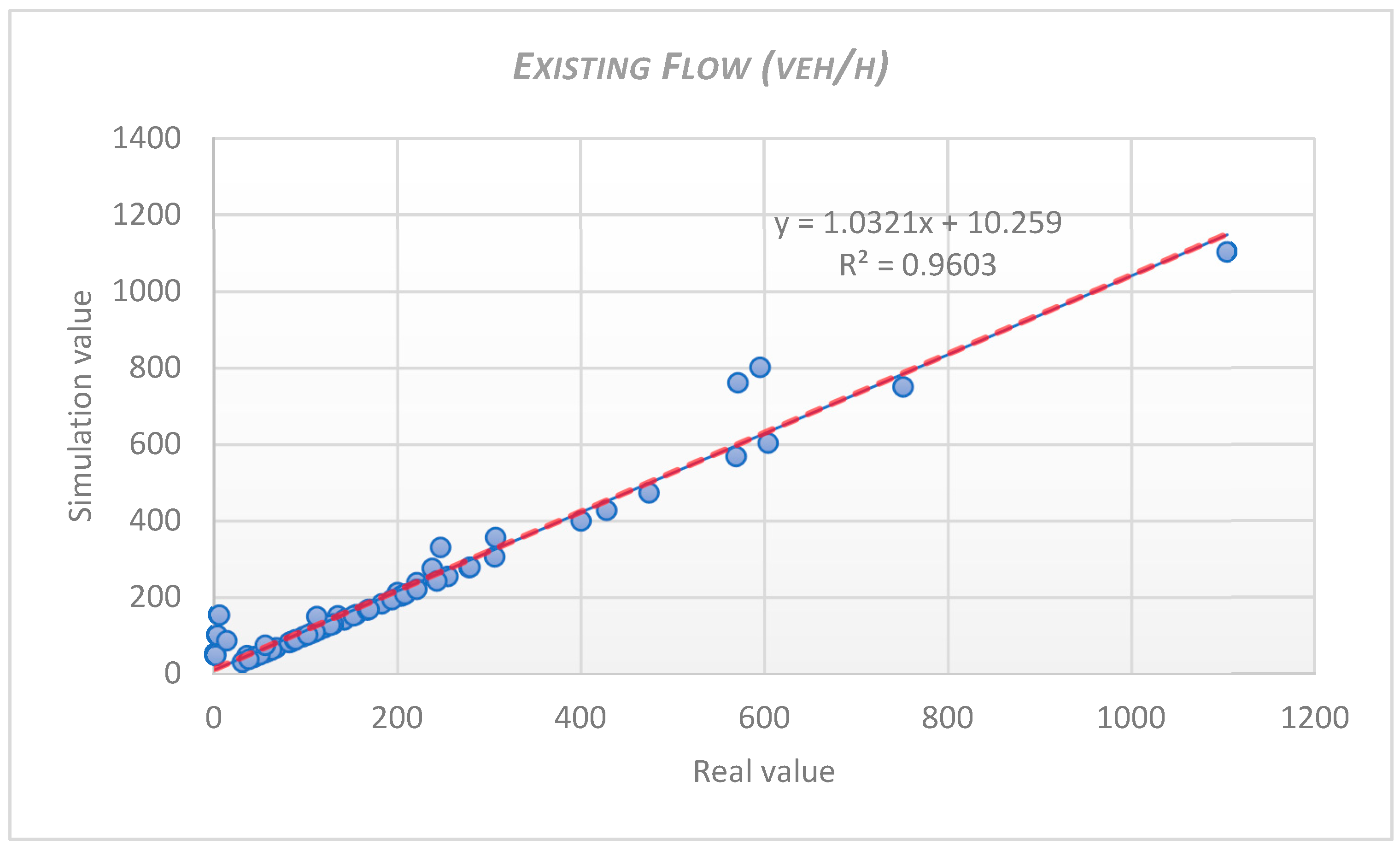
The method involves comparing traffic data collected in the field with traffic data generated by the model. The validation measure is specifically the outgoing flow from each intersection (Figure 7).

GEH Static

The GEH statistic is a formula used in traffic engineering, traffic forecasting, and traffic modeling to compare two sets of traffic volumes.
G E H = 2 ( X n s i m X n r e a l ) 2 X n s i m + X n r e a l
The GEH statistic is a valuable tool for comparing traffic volumes and avoiding the pitfalls associated with using simple percentages. Real-world transportation systems often exhibit a wide range of traffic volumes, making it challenging to establish a single acceptable percentage variation for different volumes. The non-linear nature of the GEH statistic helps address this issue by enabling the use of a single acceptance threshold across various traffic volume ranges.
In traffic modeling work, a GEH value of less than 5.0 is generally considered indicative of a good match between the modeled and observed hourly volumes. It is important to convert flows of different durations into hourly equivalents when applying these thresholds. According to DMRB guidelines, approximately 85% of the volumes in a traffic model should have a GEH value below 5.0. GEH values in the range of 5.0 to 10.0 may warrant further investigation. If the GEH value exceeds 10.0, it suggests a high likelihood of an issue with either the travel demand model or the data. This could range from simple data entry errors to more complex problems related to model calibration [45].
Our result of GEH 89% < 4 surpasses this benchmark by a significant margin (Table 3). This highlights the high degree of accuracy and reliability in our traffic modeling process. It indicates that our model has successfully accounted for the non-linear nature of traffic volumes and has effectively captured the complexities present in real-world transportation systems.

10. Results

In this section we analyze the results of our model. Table 4 represents the queue sum of the whole network in 5400 simulation seconds. The total queue of the network is computed as the sum of the queue lengths on all the links of the network during the simulation.
In both scenarios 1 and 2 (with and without transit priority), we observe a reduction in queue length. The reductions are 5,770,592 (54%) and 3,039,969 (28%) for scenario 1 and scenario 2, respectively. However, scenario 1 outperforms scenario 2 in terms of the overall reduction in queues.

10.1. Private Vehicles

In this section, we examine the waiting time and time loss for all route flows associated with each path. Figure 8 and Figure 9 illustrate the analysis of a total of 74 distinct routes. Figure 8 and Figure 9 illustrate that both scenario 1 and scenario 2, where the latter adopts priority for public transport, experience a decrease in average waiting time and time loss. However, the reduction in waiting time and time loss is more prominent in scenario 1, making it a more favorable option for private vehicles. This suggests that although scenario 2 shows improvements in the mentioned factors, the priority assignment in scenario 2 leads to a decline in performance for private vehicles when compared with scenario 1.

10.2. Emissions

Emissions represent an additional result of our simulation model. Examining the pollutants can provide valuable insights into the impact and effectiveness of any control strategy. Moreover, emissions help to illustrate the direct effects of queue length, waiting time, and time loss on the environment in a more comprehensible manner. The sum of the P M x , C O 2 , and N O x emissions is shown in the Table 5 for three different scenarios.
As can be clearly seen, the application of both scenario 1 and scenario 2 leads to a reduction in emissions for all pollutants. Scenario 1 shows more prominent decrease in emissions compared with scenario 1. Scenario 2 also results in reduced emissions; it is not as effective as scenario 1 in terms of lowering pollutant levels. This analysis is in agreement with the other analyses which were mentioned earlier.

10.3. Public Transport (Trams)

As mentioned, the artery is served by three tram lines. The table below illustrates the waiting time for the tram lines (5, 14, and 19). As is illustrated in Table 6 and the graphs above, the average waiting time in scenario 2 is the smallest compared with the other two situations.
We also calculated the overall time loss of each tram specifically for each vehicle in different directions, as shown in the charts below. The charts show the effectiveness of the algorithm in both scenarios; however, scenario 2, which assigns priority to public transit, outperforms scenario 1.
In Figure 10 we represent the average time loss of each tram line for three different scenarios. As demonstrated below, the average time loss significantly decreases in scenario 2. Although scenario 1 is also effective in reducing the time loss for all tram lines, unlike the private vehicle case, where scenario1 was more effective, here, scenario 2 excels due to transit priority.

10.4. Intersection Delay

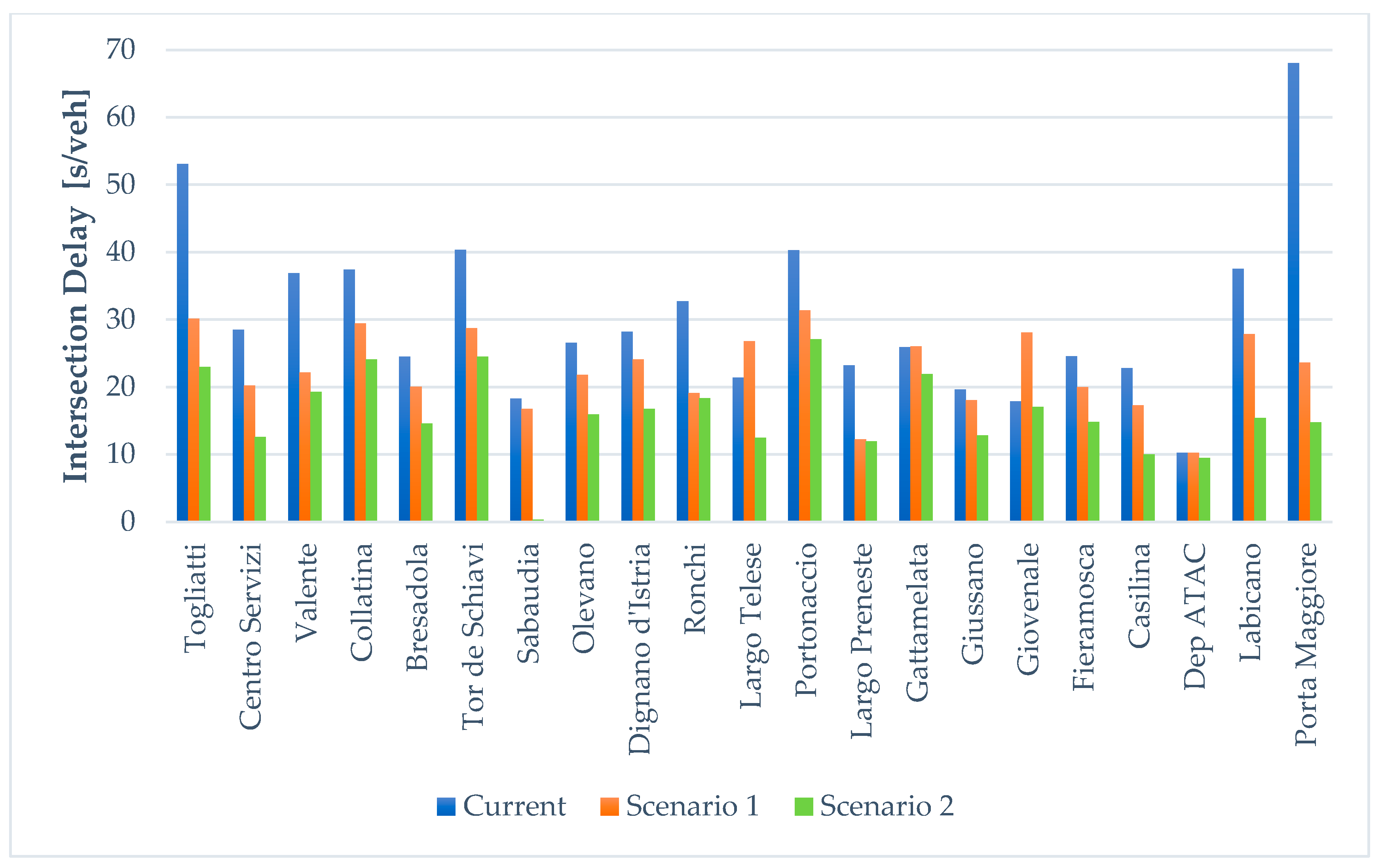
Table 7 shows the intersection delay for the 21 signalized intersections.
As shown in Table 7 and Figure 11, both scenario 1 and 2 improve the intersection delay. Yet, the overall improvement in scenario 1 is higher than in scenario 2. The results demonstrate significant performance of the algorithm, which is coherent with the previous results.

10.5. Private Vehicle vs. Public Transport

Figure 12 shows the final result comparison of private vehicles and trams in three different scenarios.
In scenario 1, where transit priority is not considered, there is a noteworthy reduction in the delay for passenger vehicles compared with the current situation, amounting to an improvement of approximately 50%. Moreover, there is also a modest improvement in tram passenger delay (around 20%). In scenario 2, which incorporates transit priority, there is a substantial improvement of 31% in tram delay when compared with the current situation. The improvement relative to scenario 1 is also noticeable (around 11%). However, it is important to note that private vehicle users experience additional delay compared with scenario 1.

11. Conclusions

Designing a road traffic management system that utilizes wireless sensor networks to improve traffic flow and reduce congestion is a complex challenge. This research study addresses the traffic light control problem using a reinforcement learning approach. By applying RL techniques, we explore a unique and innovative method for solving these challenges and achieving a more optimized and smoother traffic experience.
Through comprehensive experiments using real-world data, this study demonstrates the effectiveness of the proposed model in managing traffic light control, including cases with public transit priority. The algorithm was implemented across various intersections with different configurations, ranging from two-phase to four-phase setups. While this study does not explicitly model the interactions among intersections, it shows that the model can still learn an effective policy under rush hour traffic conditions. In scenario 1, it reduced private vehicle delay by over 50% and improved tram delay by 20% from the start of training. A comparative analysis was also conducted using scenario 2 to examine the impact of transit priority on overall network performance. In this case, tram delay was reduced by over 32%, although an increase in private vehicle delay was observed compared with scenario 1. Although the algorithm’s effectiveness in scenario 2 may appear uncertain, the primary goal of transit priority is to break the vicious cycle of congestion, encouraging a shift in mode choice toward public transportation. Due to the absence of detailed passenger data, we assumed 100 passengers per tram, which represents only 37% of tram capacity.
This study was conducted on a major corridor consisting of 21 signalized intersections and used real traffic data collected across various turning movements. It is important to note that the results obtained are comparable to those in the existing literature. For instance, a queue length reduction of approximately 50% was achieved in [18] using multi-agent reinforcement learning on a synthetic network of nine intersections, while an average delay improvement of about 30% was reported in [16] using spatiotemporal graph attention multi-agent DRL applied to real data over nine intersections.
Ultimately, field deployment is needed to gather real-world feedback and validate the proposed reinforcement learning-based approach.

Author Contributions

Conceptualization, S.M. and G.F.; methodology, S.M.; software, S.M.; validation, S.M., N.I. and G.F.; formal analysis, S.M.; investigation, S.M.; resources, G.F.; data curation, S.M.; writing—original draft preparation, S.M.; writing—review and editing, S.M., C.C., N.I. and G.F.; visualization, S.M.; supervision, G.F., C.C. and N.I.; project administration, G.F.; funding acquisition, G.F. and C.C. All authors have read and agreed to the published version of the manuscript.

Funding

National Recovery and Resilience Plan (Piano nazionale di ripresa e resilienza).

Data Availability Statement

Data is not publicly available.

Acknowledgments

Call for tender for the presentation of intervention proposals for the Strengthening of research structures and creation of R&D “national champions” on some Key Enabling Technologies to be funded under the National Recovery and Resilience Plan, Mission 4 Component 2 Investment 1.4 funded by the European Union’s NextGenerationEU.

Conflicts of Interest

The authors declare no conflict of interest.

References

  1. Mansouryar, S.; Shojaei, K.; Colombaroni, C.; Fusco, G. A Microsimulation Study of Bus Priority System with Pre-Signaling. Transp. Res. Procedia. 2024, 78, 507–514. [Google Scholar] [CrossRef]
  2. Wei, H.; Yao, H.; Zheng, G.; Li, Z. IntelliLight: A Reinforcement Learning Approach for Intelligent Traffic Light Control. In Proceedings of the ACM SIGKDD International Conference on Knowledge Discovery and Data Mining, London, UK, 19–23 August 2018. [Google Scholar]
  3. Wei, H.; Zheng, G.; Gayah, V.; Li, Z. Recent Advances in Reinforcement Learning for Traffic Signal Control: A Survey of Models and Evaluation. SIGKDD Explor. Newsl. 2021, 22, 12–18. [Google Scholar] [CrossRef]
  4. Dion, F.; Rakha, H.; Kang, Y.S. Comparison of Delay Estimates at Under-Saturated and over-Saturated Pre-Timed Signalized Intersections. Transp. Res. Part B Methodol. 2004, 38, 99–122. [Google Scholar] [CrossRef]
  5. Gershenson, C. Design and Control of Self-Organizing Systems; CopIt ArXives: Mexico City, Mexico, 2007; Volume 132. [Google Scholar]
  6. Varaiya, P. The Max-Pressure Controller for Arbitrary Networks of Signalized Intersections. In Advances in Dynamic Network Modeling in Complex Transportation Systems; Springer: New York, NY, USA, 2013. [Google Scholar]
  7. Kuyer, L.; Whiteson, S.; Bakker, B.; Vlassis, N. Multiagent Reinforcement Learning for Urban Traffic Control Using Coordination Graphs. In Machine Learning and Knowledge Discovery in Databases; Lecture Notes in Computer Science (Including Subseries Lecture Notes in Artificial Intelligence and Lecture Notes in Bioinformatics); Springer: Berlin/Heidelberg, Germany, 2008; Volume 5211. [Google Scholar]
  8. Mannion, P.; Duggan, J.; Howley, E. An Experimental Review of Reinforcement Learning Algorithms for Adaptive Traffic Signal Control. In Autonomic Road Transport Support Systems; Birkhäuser: Cham, Switzerland, 2016. [Google Scholar]
  9. Watkins, C.J.C.H.; Dayan, P. Q-Learning. Mach. Learn. 1992, 8, 279–292. [Google Scholar] [CrossRef]
  10. Balaji, P.G.; German, X.; Srinivasan, D. Urban Traffic Signal Control Using Reinforcement Learning Agents. IET Intell. Transp. Syst. 2010, 4, 177–188. [Google Scholar] [CrossRef]
  11. Arel, I.; Liu, C.; Urbanik, T.; Kohls, A.G. Reinforcement Learning-Based Multi-Agent System for Network Traffic Signal Control. IET Intell. Transp. Syst. 2010, 4, 128–135. [Google Scholar] [CrossRef]
  12. Puterman, M.L. Markov Decision Processes: Discrete Stochastic Dynamic Programming; John Wiley & Sons: Hoboken, NJ, USA, 2008. [Google Scholar]
  13. Genders, W.; Razavi, S. Using a Deep Reinforcement Learning Agent for Traffic Signal Control; John Wiley & Sons: Hoboken, NJ, USA, 2016. [Google Scholar]
  14. Mnih, V.; Kavukcuoglu, K.; Silver, D.; Rusu, A.A.; Veness, J.; Bellemare, M.G.; Graves, A.; Riedmiller, M.; Fidjeland, A.K.; Ostrovski, G.; et al. Human-Level Control through Deep Reinforcement Learning. Nature 2015, 518, 529–533. [Google Scholar] [CrossRef] [PubMed]
  15. Mazaheri, A.; Alecsandru, C. New Signal Priority Strategies to Improve Public Transit Operations in an Urban Corridor. Can. J. Civ. Eng. 2023, 50, 737–751. [Google Scholar] [CrossRef]
  16. Bie, Y.; Ji, Y.; Ma, D. Multi-Agent Deep Reinforcement Learning Collaborative Traffic Signal Control Method Considering Intersection Heterogeneity. Transp. Res. Part C Emerg. Technol. 2024, 164, 104663. [Google Scholar] [CrossRef]
  17. Li, M.; Pan, X.; Liu, C.; Li, Z. Federated Deep Reinforcement Learning-Based Urban Traffic Signal Optimal Control. Sci. Rep. 2025, 15, 11724. [Google Scholar] [CrossRef]
  18. Yu, J.; Laharotte, P.A.; Han, Y.; Leclercq, L. Decentralized Signal Control for Multi-Modal Traffic Network: A Deep Reinforcement Learning Approach. Transp. Res. Part C Emerg. Technol. 2023, 154, 104281. [Google Scholar] [CrossRef]
  19. Arulkumaran, K.; Deisenroth, M.P.; Brundage, M.; Bharath, A.A. Deep Reinforcement Learning: A Brief Survey. IEEE Signal. Process. Mag. 2017, 34, 26–38. [Google Scholar] [CrossRef]
  20. Perera, A.T.D.; Kamalaruban, P. Applications of Reinforcement Learning in Energy Systems. Renew. Sustain. Energy Rev. 2021, 137, 110618. [Google Scholar] [CrossRef]
  21. Xiao, L.; Lu, X.; Xu, T.; Zhuang, W.; Dai, H. Reinforcement Learning-Based Physical-Layer Authentication for Controller Area Networks. IEEE Trans. Inf. Forensics Secur. 2021, 16, 2535–2547. [Google Scholar] [CrossRef]
  22. Lu, X.; Xiao, L.; Xu, T.; Zhao, Y.; Tang, Y.; Zhuang, W. Reinforcement Learning Based PHY Authentication for VANETs. IEEE Trans. Veh. Technol. 2020, 69, 3068–3079. [Google Scholar] [CrossRef]
  23. Lin, Y.; Dai, X.; Li, L.; Wang, F.-Y. An Efficient Deep Reinforcement Learning Model for Urban Traffic Control. arXiv 2018, arXiv:1808.01876. [Google Scholar] [CrossRef]
  24. Bouktif, S.; Cheniki, A.; Ouni, A.; El-Sayed, H. Traffic Signal Control Based on Deep Reinforcement Learning with Simplified State and Reward Definitions. In Proceedings of the 2021 4th International Conference on Artificial Intelligence and Big Data, ICAIBD 2021, Chengdu, China, 28–31 May 2021. [Google Scholar]
  25. Bouktif, S.; Cheniki, A.; Ouni, A.; El-Sayed, H. Deep Reinforcement Learning for Traffic Signal Control with Consistent State and Reward Design Approach. Knowl. Based Syst. 2023, 267, 110440. [Google Scholar] [CrossRef]
  26. Gong, Y.; Abdel-Aty, M.; Cai, Q.; Rahman, M.S. Decentralized Network Level Adaptive Signal Control by Multi-Agent Deep Reinforcement Learning. Transp. Res. Interdiscip. Perspect. 2019, 1, 100020. [Google Scholar] [CrossRef]
  27. Liang, X.; Du, X.; Wang, G.; Han, Z. A Deep Reinforcement Learning Network for Traffic Light Cycle Control. IEEE Trans. Veh. Technol. 2019, 68, 1243–1253. [Google Scholar] [CrossRef]
  28. Zheng, G.; Zang, X.; Xu, N.; Wei, H.; Yu, Z.; Gayah, V.; Xu, K.; Li, Z. Diagnosing Reinforcement Learning for Traffic Signal Control. arXiv 2019, arXiv:1905.04716. [Google Scholar] [CrossRef]
  29. Sutton, R.S.; Barto, A.G. Reinforcement Learning: An Introduction. IEEE Trans. Neural. Netw. 2005, 9, 104281. [Google Scholar] [CrossRef]
  30. Gao, J.; Shen, Y.; Liu, J.; Ito, M.; Shiratori, N. Adaptive Traffic Signal Control: Deep Reinforcement Learning Algorithm with Experience Replay and Target Network. arXiv 2017, arXiv:1705.02755. [Google Scholar] [CrossRef]
  31. Wei, H.; Chen, C.; Zheng, G.; Wu, K.; Gayah, V.; Xu, K.; Li, Z. Presslight: Learning Max Pressure Control to Coordinate Traffic Signals in Arterial Network. In Proceedings of the ACM SIGKDD International Conference on Knowledge Discovery and Data Mining, Anchorage, AK, USA, 4–8 August 2019. [Google Scholar]
  32. Vidali, A.; Crociani, L.; Vizzari, G.; Bandini, S. A Deep Reinforcement Learning Approach to Adaptive Traffic Lights Management. In Proceedings of the CEUR Workshop Proceedings, Grosseto, Italy, 16–19 June 2019; Volume 2404. [Google Scholar]
  33. Wu, T.; Zhou, P.; Liu, K.; Yuan, Y.; Wang, X.; Huang, H.; Wu, D.O. Multi-Agent Deep Reinforcement Learning for Urban Traffic Light Control in Vehicular Networks. IEEE Trans. Veh. Technol. 2020, 69, 8243–8256. [Google Scholar] [CrossRef]
  34. Noaeen, M.; Naik, A.; Goodman, L.; Crebo, J.; Abrar, T.; Abad, Z.S.H.; Bazzan, A.L.C.; Far, B. Reinforcement Learning in Urban Network Traffic Signal Control: A Systematic Literature Review. Expert. Syst. Appl. 2022, 199, 116830. [Google Scholar] [CrossRef]
  35. Chen, R.; Fang, F.; Sadeh, N. The Real Deal: A Review of Challenges and Opportunities in Moving Reinforcement Learning-Based Traffic Signal Control Systems Towards Reality. In Proceedings of the CEUR Workshop Proceedings, Ljubljana, Slovenia, 29 November 2022; Volume 3173. [Google Scholar]
  36. Shabestary, S.M.A.; Abdulhai, B. Deep Learning vs. Discrete Reinforcement Learning for Adaptive Traffic Signal Control. In Proceedings of the IEEE Conference on Intelligent Transportation Systems, Maui, HI, USA, 4–7 November 2018; Proceedings, ITSC; Volume 2018. [Google Scholar]
  37. Li, L.; Lv, Y.; Wang, F.Y. Traffic Signal Timing via Deep Reinforcement Learning. IEEE/CAA J. Autom. Sin. 2016, 3, 247–254. [Google Scholar] [CrossRef]
  38. Kiran, B.R.; Thomas, D.M.; Parakkal, R. An Overview of Deep Learning Based Methods for Unsupervised and Semi-Supervised Anomaly Detection in Videos. J. Imaging 2018, 4, 36. [Google Scholar] [CrossRef]
  39. Ling, K.; Shalaby, A. Automated Transit Headway Control via Adaptive Signal Priority. J. Adv. Transp. 2004, 38, 45–67. [Google Scholar] [CrossRef]
  40. Long, M.; Zou, X.; Zhou, Y.; Chung, E. Deep Reinforcement Learning for Transit Signal Priority in a Connected Environment. Transp. Res. Part C Emerg. Technol. 2022, 142, 103814. [Google Scholar] [CrossRef]
  41. Chu, T.; Wang, J.; Codeca, L.; Li, Z. Multi-Agent Deep Reinforcement Learning for Large-Scale Traffic Signal Control. IEEE Trans. Intell. Transp. Syst. 2020, 21, 2901791. [Google Scholar] [CrossRef]
  42. Haarnoja, T.; Zhou, A.; Abbeel, P.; Levine, S. Soft Actor-Critic: Off-Policy Maximum Entropy Deep Reinforcement Learning with a Stochastic Actor. In Proceedings of the 35th International Conference on Machine Learning, ICML 2018, Stockholm, Sweden, 10–15 July 2018; Volume 5. [Google Scholar]
  43. Barcelo, J. Fundamentals of Traffic Simulation; Springer: New York, NY, USA, 2010; Volume 145. [Google Scholar]
  44. Krajzewicz, D.; Hertkorn, G. SUMO (Simulation of Urban MObility) An Open-Source Traffic Simulation. In Proceedings of the 4th Middle East Symposium on Simulation and Modelling, Berlin-Adlershof, Germany, 1–30 September 2002. [Google Scholar]
  45. Feldman, O. The GEH Measure and Quality of the Highway Assignment Models. In Proceedings of the Association for European Transport and Contributors, Glasgow, Scotland, 8–10 October 2012. [Google Scholar]
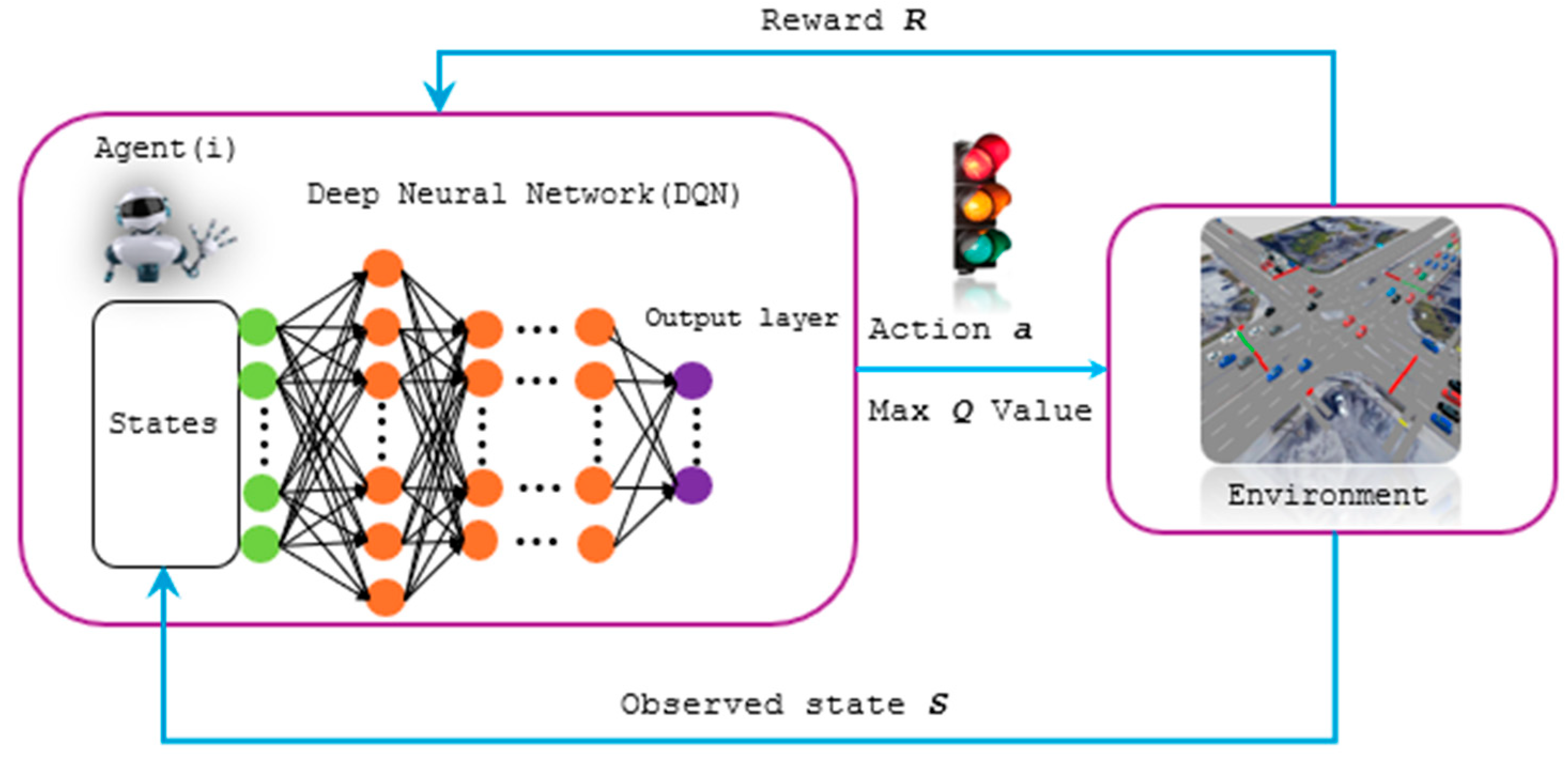
Figure 1. Reinforcement learning and deep neural network.
Futuretransp 05 00137 g001
Figure 2. Model framework.
Futuretransp 05 00137 g002
Figure 3. Q-network structure.
Futuretransp 05 00137 g003
Figure 4. The network configuration of the study area in SUMO.
Futuretransp 05 00137 g004
Figure 5. Study area (Open Street Map).
Futuretransp 05 00137 g005
Figure 6. Traffic count of major corridor.
Futuretransp 05 00137 g006
Figure 7. Goodness of fit.
Futuretransp 05 00137 g007
Figure 8. Waiting time comparison for each route flow.
Futuretransp 05 00137 g008
Figure 9. Time Loss comparison for each route flow.
Futuretransp 05 00137 g009
Figure 10. Time loss comparison for each tram line.
Futuretransp 05 00137 g010
Figure 11. Intersection delay comparison for 21 intersections.
Futuretransp 05 00137 g011
Figure 12. Network passenger delay for private vehicles and trams.
Futuretransp 05 00137 g012
Table 1. Model parameters.
Model ParameterValue
Discount factor γ0.9
Learning rate a0.001
Exploration ϵ0.05
Model update time interval4 s
Memory size20,000
Table 2. Vehicle parameters.
ParameterPassenger CarsBusesTrams
Max Speed50 km/h50 km/h50 km/h
Speed Distributionnormc (1.00, 0.10, 0.20, 2.00)normc (0.80, 0.08, 0.15, 1.50)normc (0.80, 0.08, 0.15, 1.50)
Max Acceleration2.5 m/s22.5 m/s22.5 m/s2
Max Deceleration4.5 m/s24.5 m/s24.5 m/s2
Vehicle Length4 m12 m33 m
Maximum Capacity4 people70 passengers270 passengers
Minimum Gap1.0 m1.5 m2.5 m
Car-Following ModelKraussKraussKrauss
Speed FactorDefaultDefaultDefault
Emission ModelHBEFA3/PC_G_EU4HBEFA3 (City bus profile)HBEFA3/PC_G_EU4 (Tram profile)
Traffic Flow ModelPoisson distributionFrequency headwayFrequency headway
Table 3. Validation test results.
RMSERMSPEMAPEGEH
44.77%2710.0489% < 4
Table 4. Queue sum.
Table 4. Queue sum.
CurrentScenario 1Scenario 2
10,713,723 [m]4,943,131 [m]7,673,754 [m]
Table 5. Emissions.
Table 5. Emissions.
EmissionsCurrentScenario 1Scenario 2
P M x 196.90 [Kg]113.65 [Kg]142.52 [Kg]
C O 2 9152.4 [T]6019.32 [T]7095.21 [T]
N O x 3918.75 [T]2482.90 [T]2979.57 [T]
Table 6. Average waiting time for each tram line.
Tram IDCurrentScenario 1Scenario 2
5548.67443.42318.08
14680.62507.69420.38
19377.18233.09156.64
Table 7. Intersection delay [s/veh].
IntersectionCurrent
[s]
Scenario 1
[s]
D1
[%]
Scenario 2
[s]
D2
[%]
Togliati5325533043
Centro servizi2813542029
Valente3619472239
Collatina3723382922
Bresadola2413462017
Tor de schiavi4025382830
Sabaudia188561611
Olevano2615422119
Dignano d’istia2816432414
Ronchi3219411941
Largo telese21143326−24
Portonaccio4027323123
Largo preneste2312481248
Gattamelata25202026−4
Giussano191237185
Giovenale1717028−65
Fieramosca2413462017
Casilina229591723
Dep Atac10910100
Labicano3715592727
Porta maggiore6816762366
Disclaimer/Publisher’s Note: The statements, opinions and data contained in all publications are solely those of the individual author(s) and contributor(s) and not of MDPI and/or the editor(s). MDPI and/or the editor(s) disclaim responsibility for any injury to people or property resulting from any ideas, methods, instructions or products referred to in the content.