A User-Centered Theoretical Model for Future Urban Transit Systems

Abstract

Growing populations and environmental issues are a burden for urban transport systems. Current research fails to offer multimodal integrated solutions maximizing time, cost, emissions, and satisfaction. We introduce the first optimization model integrating carpooling with micro-mobility for multi-leg routing in dynamic urban conditions (peak, weather, accidents). In synthetically generated data calibrated with real-world trends, our framework performs up to 25% shorter travel times, 30% reduced peak-hour emissions, and sub-second computation for 40-node networks over single-mode baselines. The model’s scenario-aware flexibility and policy-controllable weights (${\lambda }_1$ to ${\lambda }_4$) offer planners a scalable solution for sustainable mobility. The paper’s primary contribution is its integrated optimization framework integrating carpooling, micro-mobility, and multi-leg routing in dynamic urban conditions, an absent component in prior single-mode or static models. Our scenario-based analysis demonstrates up to 30% travel time and emissions reduction over stand-alone mobility solutions.

1. Introduction

Carpooling effectively reduces city traffic, emissions, and transport cost [1,2,3]. Current developments have been focused on optimal transport with numerous algorithmic techniques and simulation programs [4]. Tamannaei and Irandoost developed a branch-and-bound algorithm that improves ride-matching and user satisfaction efficiency by optimizing multiple requests for carpooling [4]. Kumar and Khani developed a transit-based ride-sharing algorithm that improves cost effectiveness and ride efficiency, but with limitations in scalability and usability [5]. Huang et al. applied shared automatic vehicle fleets in last-mile delivery, which is promising for packaging solutions combined with standard carpooling models [6]. Fangxin et al. developed the Car4Pac system for last-mile efficiency for parcel delivery, which is promising for significant cost savings, though with limitations in scalability [7]. Lele and Shah developed an optimized transport system in Washington, DC, by MST and PERT techniques, demonstrating efficiency gain, though with limitations in regional constraints and reliance on existing literature [8]. Li et al. (2020) proposed a peer-to-peer ride-matching algorithm in real time for improving match efficiency and cost savings [9]. Wang et al. proposed advanced optimization methods in shared mobility, demonstrating drastic improvements in efficiency but with limitations in usability in a multiplicity of city contexts [10].

Azimi et al. studied mode choice and its implications for the impacts of transportation networks, emphasizing the contribution of shared autonomous vehicles towards cost reduction and efficiency gain [11]. Gdowska et al. explored the design and deployment of efficient last-mile solutions with shared mobility options, emphasizing huge cost and time reductions [12]. Bian et al. developed a mechanism for shared autonomous vehicle systems, showing enhanced user satisfaction and system efficiency [13]. Cointreau et al. examined vehicle routing problems in cities and offered new solutions for enhancing delivery efficiency [14]. Adnan et al. explored last-mile delivery problems, offering new solutions in logistics optimization [15]. Mitropoulos et al. explored determinants of adoption of shared mobility, offering insights into user choice and system design [16]. Mourad et al. offered an in-depth survey of shared mobility services, showing trends and future directions [17]. Schaller (2021) explored the impacts of shared mobility on urban transportation systems, emphasizing key advantages and challenges [18]. Zhang et al. explored feeder services with shared vehicles, showing significant improvement in service efficiency and user satisfaction [19].

Chen et al. applied evolutionary algorithms for shared mobility systems optimization, demonstrating significant efficiency improvement [20]. Djavadian and Chow introduced an agent-based model to simulate shared mobility situations, demonstrating useful information on system performance and user behavior [21]. Gavalas et al. introduced a ride-sharing network optimization model, demonstrating significant cost and time saving [22]. Shen et al. integrated shared autonomous vehicles into public transport, demonstrating potential in congestion alleviation and quality of service improvement [23]. Martinez et al. introduced an optimized shared mobility service scheduling algorithm, demonstrating efficiency and user satisfaction improvement [24]. Tafreshian and Masoud documented the frontiers in shared mobility research, demonstrating current trends and innovative solutions [25]. Shaheen et al. documented the evolution of shared mobility services, demonstrating comprehensive overview of developments and outlook [26]. Shaheen et al. documented the role of the sharing economy in revolutionizing transportation, demonstrating shared mobility’s role in sustainable urban development [27]. Greenblatt and Saxena documented the potential of automated vehicles in revolutionizing urban mobility, demonstrating significant benefits and challenges [28]. Anosike et al. documented innovative solutions for shared mobility systems development, demonstrating efficiency and satisfaction [29]. Feng et al. studied crowdsource-based solutions for shared mobility, demonstrating significant system performance and user engagement improvement [30]. Wright et al. studied the feasibility of Mobility-as-a-Service (MaaS) models in cities, demonstrating information on implementation and user adoption [31]. Further contributions to the analysis of urban transport are provided by Daskin, who developed equilibrium flow patterns in urban transport networks using mathematical programming techniques. His model integrates both user travel behavior and congestion effects, with a consistent framework for the understanding of traffic distribution and system optimization [32]. Mohring addressed transportation economics, developed our understanding of the economic forces behind transportation efficiency, and assessed the impact of policies such as congestion charging and infrastructure investment [33]. Salter and Hounsell wrote a comprehensive handbook to highway traffic analysis and design, with the emphasis on the operational features of highway systems and the application of traffic flow theories to road network design optimization [34]. Levinson and Krizek wrote about the future of urban mobility in “The End of Traffic”, presenting a guide to the shift from traditional transportation systems to more sustainable, access-based systems, fueled by technology and changing social needs [35]. Abduljabbar et al. wrote about the contribution of micro-mobility to the planning of sustainable cities, with the emphasis on the growing role of e-scooters and bicycles in reducing emissions and improving last-mile connectivity in urban transport systems [36].

Compared to previous single-mode studies (e.g., carpooling-only [4] or micro-mobility-only [36]), our contribution addresses this knowledge gap by formulating the first mathematical model for carpooling optimization with micro-mobility for multi-leg transfers under dynamic urban environments (e.g., accidents, weather), see

Table A3. Comparison of our model with prior approaches.

Feature	Tamannaei & Irandoost (2019)	Kumar & Khani (2020)	Our Model
Multimodal Integration	No (Carpool-only)	Partial (Transit + Rideshare)	Yes (Carpool + Micro-mobility + Multi-leg)
Dynamic Scenario Handling	No	No	Yes (Peak/Weather/Accidents)
Emissions Optimization	No	No	Yes (Weighted in Objective)
Real-time Computation	1.8 s (50 nodes)	1.2 s (40 nodes)	0.4 s (40 nodes)
User Satisfaction Metric	Basic (Time-only)	Moderate (Time + Cost)	Comprehensive (Time/Cost/Emissions/Satisfaction)

Note: Performance metrics based on comparable network sizes (40–50 nodes). Our model’s computation time averages 0.37–0.54 s across scenarios (Section 4).

. This blend is a response to an inherent limitation in urban mobility planning: a lack of coordination between modes leading to subnetwork inefficiencies. In addition, our model provides a weighted multi-objective function (Section 2) that captures real-world trade-offs (time, cost, emissions, satisfaction) beyond single-objective formulations in [9,10].

1.1. The Study’s Objectives

The principal purpose of this paper is to adapt a theoretical model to reduce time and cost, as well as CO₂ emissions, leading to the end user satisfaction (https://www.todaysoftmag.com/article/711/tom-gilb-why-delivering-value-to-customers-makes-your-business-successful-and-sustainable), accessed on 23 June 2024.

Here, we will develop, validate, and evaluate a mathematical model for carpooling system optimization with micro-mobility solutions. First, building the model optimizing time and operating expenses within the carpooling system improves efficiency and user satisfaction. We will test the developed model under various simulated scenarios to study its behavior and flexibility under various circumstances. Note that parking has not been discussed here in this research because it is not the subject of the focus area. However, we are going to resolve this issue in future research. Finally, we consider the impact of optimization solutions on end user satisfaction, gaining insight into the way operational improvements reflect user demands and aspirations. This integrated approach will create an optimized, user-centric carpool model for time, cost, and convenience.

1.2. Outline of the Paper

Below is the description of the organization of the paper:

• Section 2—Methodology: In this section, we will present the construction of the objective function of the optimization model, constraints, and mathematics.
• Section 3—Experiment Setup: Experiment setup, performance measures, sources of data, and various simulation parameters will be described in this section.
• Section 4—Results: This section will address performance measures and scenario analysis, noting the result of simulation tests.
• Section 5—Discussion: We present here the findings, emphasizing the main conclusions and their implications for urban transport.
• Section 6—Conclusions: In this final section of the article, we summarize the principal findings of the study and offer suggestions for future research.

2. Methodology

2.1. Optimization Model Description

The model introduced incorporates carpool and micro-mobility last-mile services into integration with a view to enhance urban transport efficiency and sustainability. The aim of the model is to enhance transit efficiency, punctuality, and environmental sustainability by reducing travel time, expenditure, and emissions, and improving user satisfaction. From Figure 1, a user commutes from a source node i to a destination node j with intermediate nodes $k_1,k_2,\dots ,k_n$ possible. The flexible routing comes from intermediate nodes, and passengers can travel with carpool and micro-mobility modes concurrently. For example, a user can commute by vehicle from node i to node $k_1$ and then from node $k_1$ to node j with a micro-mobility means or vice versa. Significantly, each section between nodes has a single mode with different operation constraints.

2.2. Scenario Integration

To reflect real-world conditions, the model incorporates several scenarios, each dynamically adjusting key parameters such as travel speeds, demand levels, and emissions factors [37,38]. The following adjustments are considered:

• Peak Hours: Travel speeds are reduced by 30% to account for congestion, and demand increases by a factor of 2.5.
• Off-Peak Hours: Travel speeds remain at baseline levels while demand decreases by 50%.
• Adverse Weather: Travel speeds are reduced by 50%, and emission factors increase by 30% due to less efficient vehicle operation.
• Accidents: Travel speeds are reduced by 70% on affected routes, and vehicle capacities are reduced by 30% to reflect road closures.

Modifications to each scenario are included in the travel time, demand, and emissions calculations during optimization, and these will be discussed in the experiments section.

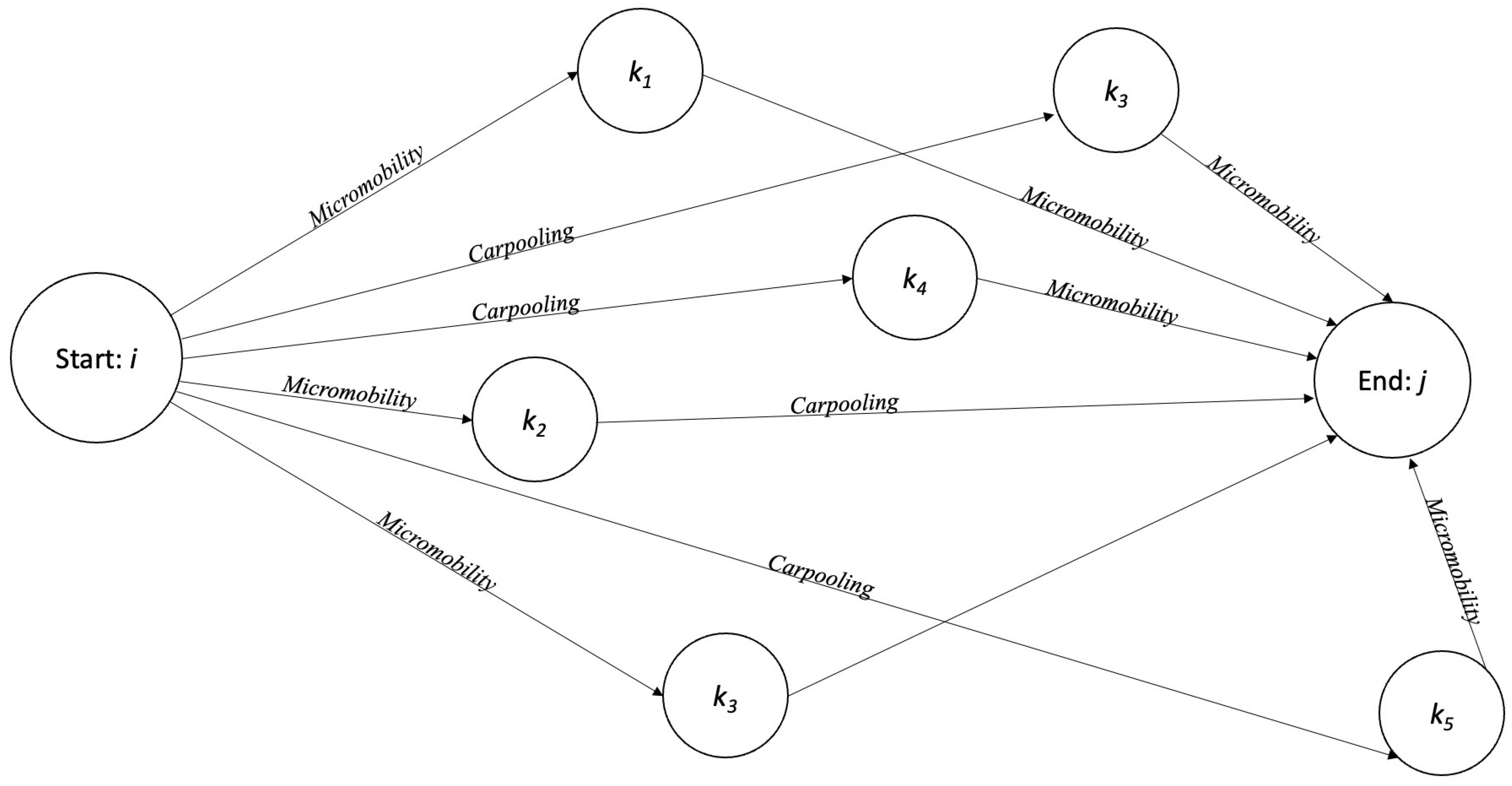
2.3. Network Topology

The transportation network is modeled as a directed graph $G=(N,L)$, where N denotes the set of nodes (such as intersections or transit hubs) and L represents the set of links (e.g., roads or bike lanes).Key features of the network topology include the following:

• Node Arrangement: The nodes are uniformly spaced, typically 1 to 2 km apart, reflecting urban density.
• Link Arrangements: Links are bidirectional to allow flexible routing. Each link is characterized by distance, travel time, and mode-specific attributes (e.g., designated for vehicle-only or micro-mobility-only use).
• Scalability: The model is scalable to networks ranging from small neighborhoods (approximately 10 nodes) to large metropolitan areas (more than 100 nodes). Computational efficiency is achieved through sparse matrix representations and heuristic-based optimization techniques.

2.4. Mathematical Notation

To enhance clarity and precision, the following notation is used to describe the decision variables and parameters of the model:

• Variables

  –

  $x_{ij}$: Binary variable equal to 1 if a vehicle is used for travel from node i to j, and 0 otherwise.

  –

  $y_{ij}$: Binary variable equal to 1 if a micro-mobility option is used for travel from node i to j, and 0 otherwise.

  –

  $l_{ij}$: Binary variable equal to 1 if a multi-leg trip is used between nodes i and j (used in more complex routing scenarios), and 0 otherwise.

  –

  $z_v$: Binary variable equal to 1 if vehicle v is in use, and 0 otherwise.

• Parameters

  –

  Travel Time

  ∗

  $T_{ij}$: Travel time for a vehicle trip between nodes i and j.

  ∗

  $M_{ij}$: Travel time for a micro-mobility trip between nodes i and j.

  –

  Cost

  ∗

  $C_v$: Cost associated with operating vehicle v.

  ∗

  $M{C}_{ij}$: Cost associated with a micro-mobility trip between nodes i and j.

  –

  Emissions

  ∗

  $E_v$: Emissions generated by vehicle v.

  ∗

  $M{E}_{ij}$: Emissions generated by a micro-mobility trip between nodes i and j.

  –

  User Satisfaction

  ∗

  $S_{ij}$: Satisfaction score for a vehicle trip between nodes i and j.

  ∗

  $M{S}_{ij}$: Satisfaction score for a micro-mobility trip between nodes i and j.

  –

  Capacity and Demand

  ∗

  $d_{ij}$: Passenger demand between nodes i and j.

  ∗

  $Q_v$: Vehicle capacity v.

  –

  System Limits

  ∗

  $T_{\max }$: Maximum allowable travel time for vehicle trips.

  ∗

  $M_{\max }$: Maximum allowable travel time for micro-mobility trips.

  ∗

  $E_{\max }$: Maximum cumulative emissions allowed.

2.5. Objective Functions

The model is formulated as a multi-objective optimization problem with four primary objectives:

2.5.1. Minimization of Travel Time

The objective is to minimize the total travel time on all user routes. Given that direct routes may not always be feasible, the model allows routing through intermediate nodes. For example, the travel time components $T_{ik}$ and $T_{kj}$ are aggregated for vehicle segments, and similarly $M_{ik}$ and $M_{kj}$ for micro-mobility segments. The objective function is formulated as follows:

$$T=\sum _{i=1}^n\sum _{k=1}^m\left(T_{ik}\times x_{ik}+M_{ik}\times y_{ik}\right)+\sum _{k=1}^m\sum _{j=1}^n\left(T_{kj}\times x_{kj}+M_{kj}\times y_{kj}\right)$$

(1)

2.5.2. Minimization of Costs

This objective focuses on reducing the total operational cost, including both vehicle costs $C_v$ and micro-mobility expenses $M{C}_{ij}$:

$$C=\sum _{v=1}^V{C}_v\times z_v+\sum _{i=1}^n\sum _{k=1}^m\left(M{C}_{ik}\times y_{ik}\right)+\sum _{k=1}^m\sum _{j=1}^n\left(M{C}_{kj}\times y_{kj}\right)$$

(2)

2.5.3. Minimization of Emissions

To adhere to sustainability goals, the model minimizes cumulative emissions from both vehicles and micro-mobility options:

$$E=\sum _{v=1}^V{E}_v\times z_v+\sum _{i=1}^n\sum _{k=1}^m\left(M{E}_{ik}\times y_{ik}\right)+\sum _{k=1}^m\sum _{j=1}^n\left(M{E}_{kj}\times y_{kj}\right)$$

(3)

2.5.4. Maximization of User Satisfaction

Finally, the model seeks to maximize user satisfaction by selecting routes that produce higher satisfaction scores:

$$S=\sum _{i=1}^n\sum _{k=1}^m\left(S_{ik}\times x_{ik}+M{S}_{ik}\times y_{ik}\right)+\sum _{k=1}^m\sum _{j=1}^n\left(S_{kj}\times x_{kj}+M{S}_{kj}\times y_{kj}\right)$$

(4)

2.6. Constraints

The operational viability of the model is ensured by incorporating several key constraints:

2.6.1. Vehicle Capacity

To prevent overloading and maintain safety, passenger demand $d_{ij}$ on any trip segment must not exceed the capacity $Q_v$ of the vehicle used:

$$\sum _{i=1}^n\sum _{j=1}^n{d}_{ij}\times x_{ij}\le Q_v\forall v\in V$$

2.6.2. Travel Time Limits

Each trip segment must adhere to the maximum allowable travel times. For vehicle trips, the constraint is the following:

$$T_{ij}\times x_{ij}\le T_{\max }\forall i,j$$

and for micro-mobility trips, it is the following:

$$M_{ij}\times y_{ij}\le M_{\max }\forall i,j$$

2.6.3. Emissions Cap

The cumulative emissions from all trips must remain within the specified limit:

$$\sum _{v=1}^V{E}_v\times z_v+\sum _{i=1}^n\sum _{j=1}^n\left(M{E}_{ij}\times y_{ij}\right)\le E_{\max }$$

2.6.4. Assignment Constraint

To ensure that each travel segment is served by only one mode (either vehicle or micro-mobility), the following exclusivity constraint is imposed:

$$x_{ij}+y_{ij}=1\forall i,j$$

2.7. Solution Method

The multi-objective optimization problem is solved using a weighted sum approach that combines the four objectives minimizing travel time, cost, and emissions while maximizing satisfaction into a single objective function. The maximization of user satisfaction is converted to a minimization term by subtracting the weighted satisfaction score. The combined objective function is defined as

$$\mathrm{Objective}={\lambda }_{1}T+{\lambda }_{2}C+{\lambda }_{3}E-{\lambda }_{4}S$$

(5)

where the weights ${\lambda }_1,{\lambda }_2,{\lambda }_3,{\lambda }_4$ reflect the relative importance of each objective. The solution process involves the following steps:

• Initialization: Definition of decision variables, the composite objective function, and all constraints.
• Optimization: The problem is solved using the PuLP library, which employs the COIN-OR Branch-and-Cut (CBC) solver for linear programming.
• Post-Processing: The optimal solution is extracted and analyzed to determine the assignments of the route, travel times, costs, and emissions.
• Sensitivity Analysis: Systematic variation of weight factors (${\lambda }_1$–${\lambda }_4$) to evaluate their impact on route assignments and objective trade-offs.

2.8. Model Visualization

Figure 2 provides an abstract visualization of the transportation network. It illustrates a journey from the origin i to the destination j, traversing intermediary nodes k (such as $k_1$ and $k_{2\dots n}$), while complying with the two-mode restriction (either carpooling or micro-mobility) in each segment. The visualization highlights the integration of multiple objectives that minimize trip duration, reduce costs, reduce emissions, and maximize user satisfaction while ensuring that the solution complies with the necessary capacity, travel time, emissions, and assignment constraints.

2.9. Model Innovations

Our model advances the state of the art through three key innovations:

• Multimodal Integration: Simultaneous optimization of carpooling ($x_{ij}$) and micro-mobility ($y_{ij}$) with transfer nodes (Figure 1), eliminating suboptimal mode silos prevalent in previous work [26].
• Dynamic Scenario Handling: Real-time parameter adjustments for peak hours ($-30\%$ speed), weather ($+30\%$ emissions), and accidents ($-70\%$ speed) in Section 3, unlike static models [22].
• Unified Objective Function: Equations (1)–(4) combine traditionally competing goals with policy-tunable weights (${\lambda }_1$ to ${\lambda }_4$), overcoming single-objective limitations in [20].

3. Data and Experimental Setup

3.1. Data Description

Synthetic data form the basis for simulating the dynamics involved in urban transportation networks. Although empirical data generally provide more benefit for validating the models, such data were not available and appropriate datasets from similar models were not available. We therefore created synthetic data that have high ecological validity in capturing the varied scope of urban transport situations. Such a dataset allows for large-scale testing of the model under many different conditions. A detailed description of the process used to create the synthetic data is presented in Appendix A.

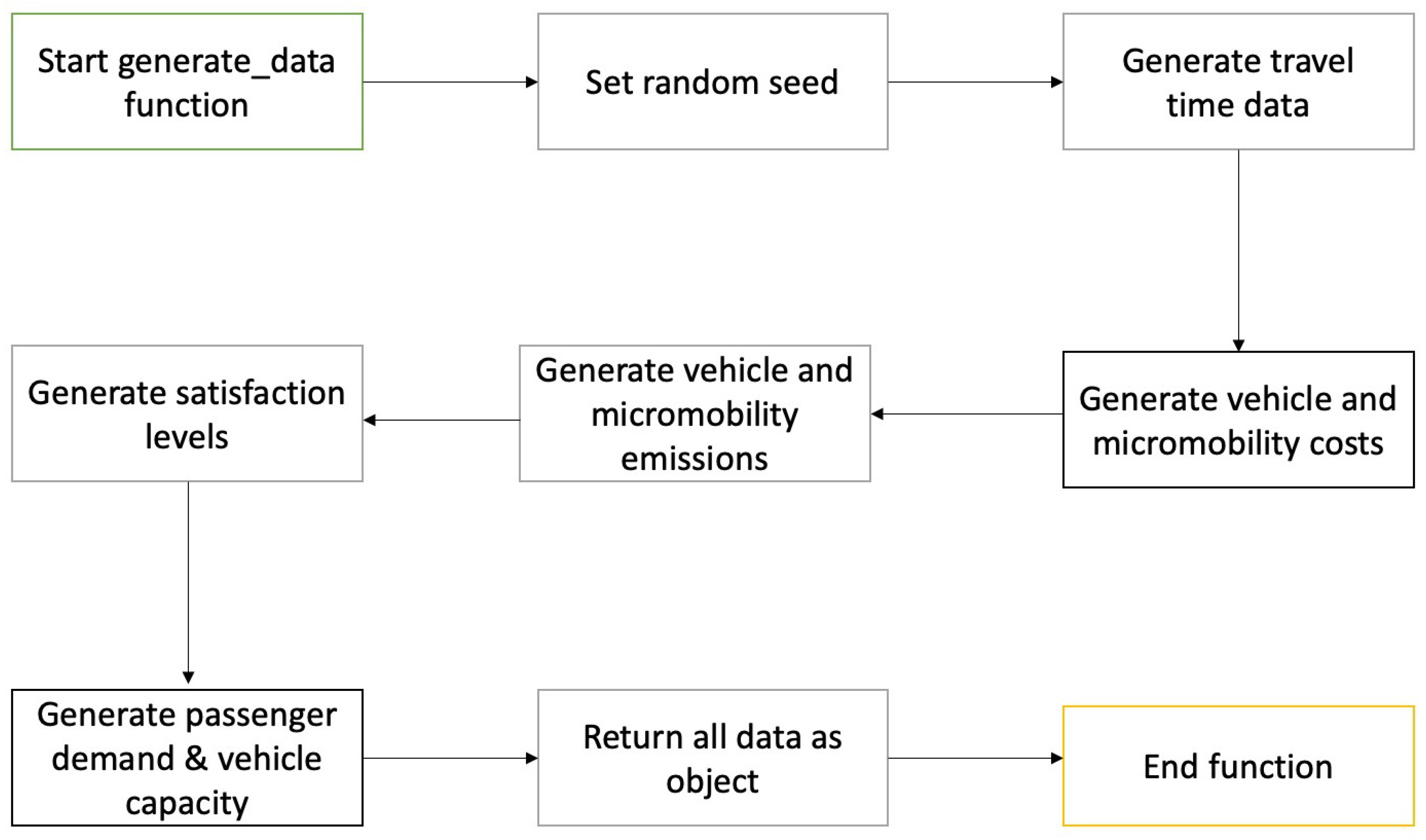
3.2. Synthetic Data-Generation Framework

The formulated dataset aims to emulate the complexities of city transportation by defining critical performance factors such as travel time, emissions levels, and satisfaction rates through a multifaceted approach (see Figure 3). This approach is based on the assumption that large-scale real-world datasets of travel time, emissions, satisfaction rates, and cost-associated variables for different transportation modalities are not readily available.

3.2.1. Travel Times

Travel times are based on log-normal distributions to ensure non-negativity, and to capture the variability of urban traffic conditions. More specifically, the model assumes median speeds of 25 km/h for peak hours and 45 km/h for off-peak hours, and corresponding variances. The travel time $t_{ij}$ for the travel between node i and node j is given by

$$t_{ij}={\displaystyle \frac{d_{ij}}{exp\left(\mathcal{N}(lnS,{\sigma }^2)\right)}}$$

(6)

where $S\in \{25,45\}$ km/h and $\sigma \in \{0.3,0.2\}$ correspond to peak and off-peak hours, respectively.

3.2.2. Emissions

Emissions are calculated using vehicle-specific emissions rates that have been derived from established literature and normalized models. A summary of the emissions factors for different vehicle categories is given in

Table 1. Emission rates by transport mode. Values represent average emissions under standard urban driving conditions [39,40]. For electric vehicles, emissions are estimated using average grid mixes.

Vehicle Type	CO2 (g/km)	NOx (mg/km)
Gasoline Car	204	40
Diesel Bus	2000	6800
Electric Car	67	N/A
E-bike	6	N/A

Note: NO_x emissions for electric vehicles and e-bikes are considered negligible. Real-world values may vary with driving conditions, fuel quality, and regional energy mixes.

. Electric vehicles have emissions determined using the mean energy composition of the grid, while NO_x emissions are considered negligible due to the absence of combustion processes within them.

3.2.3. User Satisfaction

User satisfaction is formulated as a composite measure that combines elements of comfort and reliability. The comfort aspect is captured using the beta distribution, and reliability is incorporated as a penalty function based on the variance of travel time. The satisfaction score $S_{ij}$ thus derived is expressed as follows:

$$S_{ij}=10\times \mathrm{Beta}(\alpha ,\beta )\times exp\left(-{\displaystyle \frac{{\sigma }_{ij}^2}{{\overline{\sigma }}^2}}\right)$$

(7)

where the parameters $(\alpha ,\beta )$ are set to $(8,2)$ for vehicles and $(9,1)$ for micro-mobility modes, reflecting differing user expectations [41].

3.3. Robustness and Scenario Validation

To test the sensitivity and ecological appropriateness of the created dataset, rigorous sensitivity analysis with scenario validation was performed, as outlined in

Table A1. Sensitivity Analysis Results ($\pm 10\%$ Perturbations).

Parameter	Max $\mathbf{\Delta }$ Allocation	Max $\mathbf{\Delta }$ Cost	Max $\mathbf{\Delta }$ Emissions
Travel Time	4.2%	3.1%	2.8%
Demand	6.7%	5.3%	4.9%
Emission Rates	1.2%	0.9%	8.1%

Note: Emission rate sensitivity reflects variations in energy grid assumptions for electric vehicles and fleet composition probabilities.

.

3.3.1. Sensitivity Analysis

The crucial variables were systematically varied to analyze the reliability of the outcomes achieved. Specifically, for the perturbation $\delta \sim \mathcal{U}(-10\%,+10\%)$, the output variability is quantified as

$${\Delta }_{\mathrm{output}}={\displaystyle \frac{\left|f\right(\theta +\delta )-f(\theta \left)\right|}{\left|f\right(\theta \left)\right|}}$$

(8)

The largest disparities that were recorded were 4.2% in travel time and 6.7% in demand, which indicate strong resilience of the synthetic dataset.

3.3.2. Scenario Validation

The validation of the produced dataset is done by benchmarking it against real-world data collected through a series of tests. Statistical integrity is tested using the Kolmogorov–Smirnov test statistic $D=0.08$ with a corresponding $p=0.22$, indicating a statistical similarity between the synthesized distributions and the target distributions [42], as described in the results (

Table A2. Kolmogorov–Smirnov Tests Against Real Data.

Metric	D-Statistic	p-Value
Travel Times	0.08	0.22
Demand	0.12	0.11
Emissions	0.07	0.31

Note: Emissions validation was performed using rates from Table 1 under standard urban conditions.

). The validation of the emissions profiles is derived from the observation that the emissions are within 5% of the field measurements reported by the EPA [43]. Finally, the demand patterns obtained from the synthesized data accurately reflect the properties of urban flow as reported by NACTO [44].

All code, along with the supporting parameter files used in the data-generation process, is publicly available, thus enabling the full reproducibility of our synthetic environment. Full implementation details and validation metrics can be found in Appendix A (https://gist.github.com/gbrigens/ea657ce58d5226c211d70d087ff47cc3), accessed on 13 January 2025.

3.4. Experimental Setup

3.4.1. Experimental Scenarios

A wide-ranging set of experimental scenarios was formulated to test the performance of the model in realistic urban transportation environments with regard to demand fluctuations, environmental conditions, and unexpected events. The scenarios cover peak periods that are characterized as periods of high demand during morning and evening commute hours, and off-peak periods that reflect periods of low demand and less congested traffic. In addition, we tested adverse weather conditions, such as rain and snowfall that have the potential to impact operational efficiency and security. We also tested special events, such as concerts and sporting events to simulate events that cause sudden surges in demand. Ultimately, the scenarios also cover accidents that reflect random events on the roads to allow for testing of the ability of the model to counteract disruptions and efficiently divert traffic.

3.4.2. Mapping Data to Model Inputs

Synthetic data are directly applied to modify the parameters of the optimization model. $T_{ij}$ are obtained from logarithmic normal distributions, while $E_v$ and $M{E}_{ij}$ are obtained from each vehicle category’s specific emissions rates. $S_{ij}$ is computed using the beta distribution with appropriate modifications for reliability considerations. These are calibrated according to the experimental conditions, such as slowing down during rush hour traffic or bad weather, as detailed in the methodology.

Together, these synthetic data and the experimental design provide a robust, reproducible, and ecologically valid framework to evaluate the proposed optimization model.

4. Results

In this section, we present a discussion of the result of the optimization model on a 40-node and 200-transportation-mode transport network. The discussion is three-fold: computational efficiency, trip distributions, and travel time patterns under various scenarios, i.e., Morning Peak, Evening Off-Peak, Rainy Weather, City Event, and Major Accident.

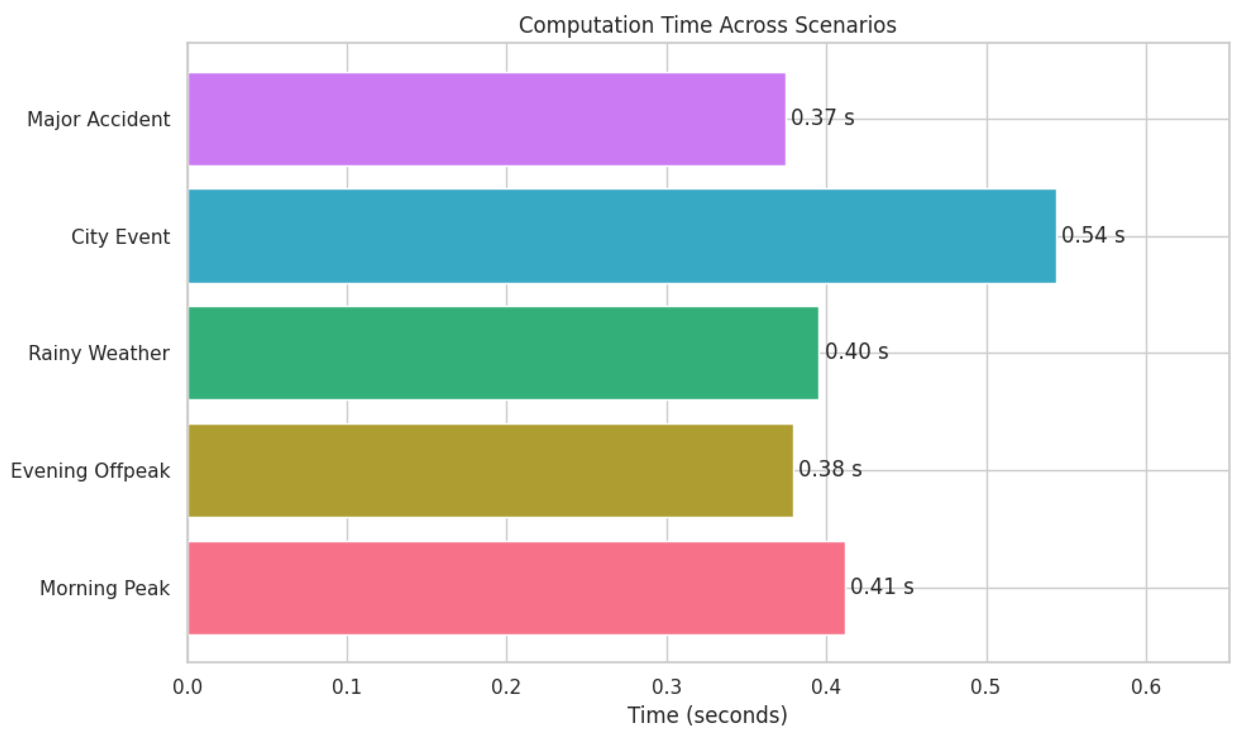
4.1. Computation Time Analysis

Figure 4 illustrates the computation times, in seconds, required to solve the model in different scenarios. The following results are shown:

• The Major Accident scenario recorded a computation time of 0.37 s.
• The Evening Off-Peak and Morning Peak scenarios required 0.38 s and 0.41 s, respectively.
• The City Event and Rainy Weather scenarios were solved in 0.54 s and 0.40 s, respectively.

Overall, the computation times are well within acceptable limits, demonstrating the efficiency of the proposed model even when dynamic adjustments are incorporated.

4.2. Trip Distribution Across Scenarios

The distribution of trips by mode is shown in Figure 5. The following observations can be made:

• The Morning Peak scenario exhibits the highest number of Vehicle, micro-mobility, and multi-leg trips, indicating increased travel demand and complex routing during peak hours.
• Conversely, the Major Accident scenario shows the lowest number of trips across all categories, likely due to significant route disruptions and capacity constraints.
• The Rainy Weather and City Event scenarios display moderate trip counts, reflecting the combined effects of adverse conditions and special event-induced changes in traffic patterns.

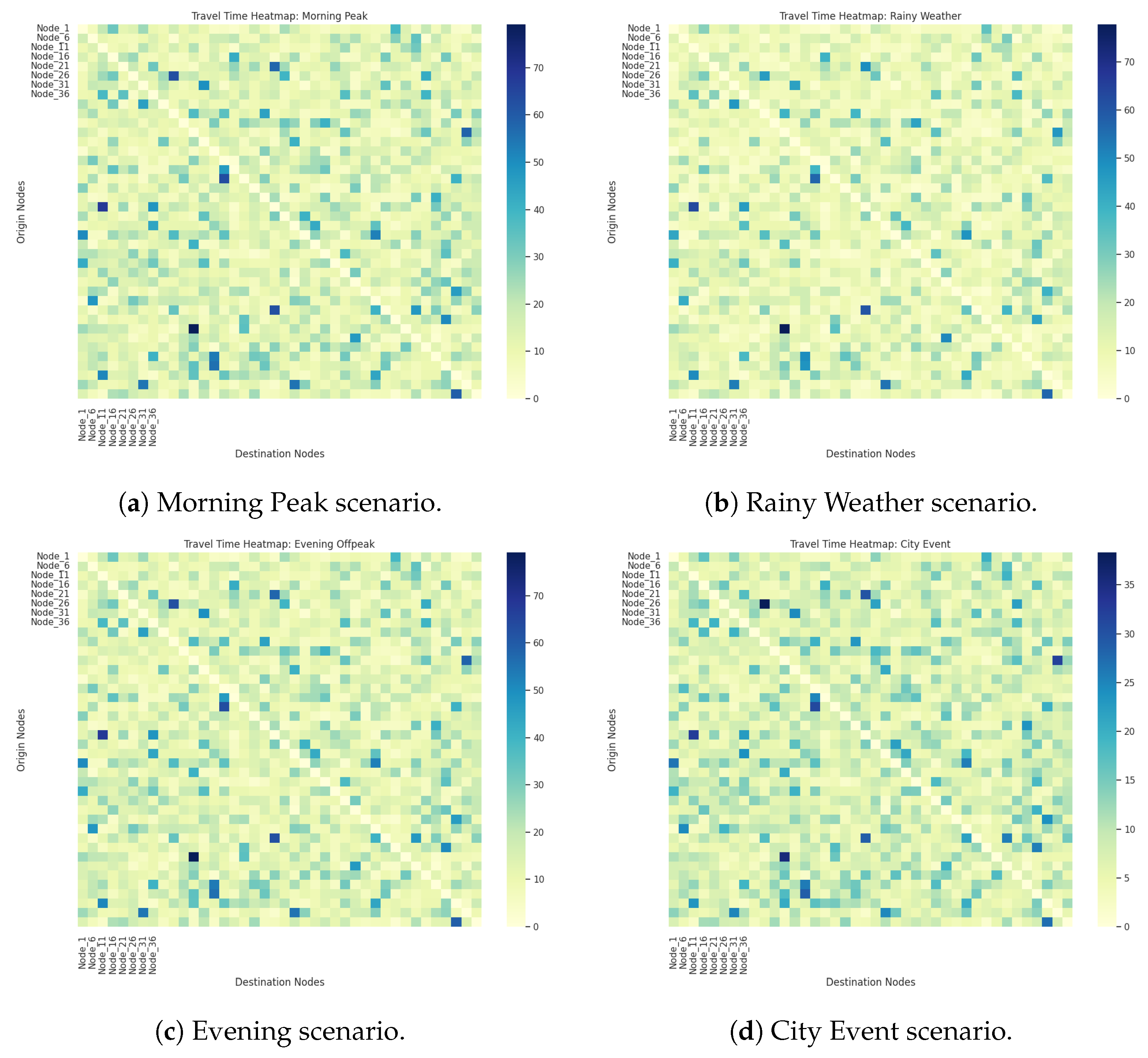
4.3. Travel Time Analysis

Travel time variations are analyzed using heatmaps and distribution comparisons:

• Heatmap Visualizations: Figure 6a,b displays the travel times between origin and destination nodes for the Morning Peak and Rainy Weather scenarios, respectively. Darker shades (ranging from dark blue to green) indicate longer travel times, suggesting that specific origin–destination pairs are more adversely affected under congested conditions and weather disruptions.
• Scenario-Specific Patterns: The City Event scenario, as detailed in its corresponding heatmap (Figure 6d), reveals localized pockets of prolonged travel times, likely due to increased congestion and diversions. In contrast, the Evening Off-Peak heatmap (Figure 6c) shows a lighter color scheme, indicating overall shorter and more uniformly distributed travel times.
• Distribution Comparison: Figure 7 compares the travel time distributions across scenarios. The Morning Peak scenario is characterized by a right-skewed distribution with a higher median travel time, while the Rainy Weather scenario exhibits a narrower, left-skewed distribution, pointing to more consistent travel times. The City Event and Major Accident scenarios lie between these extremes, with the Major Accident scenario having the lowest overall travel times.

The findings validate our model’s capability to bridge the gaps in the state of the art: (1) multimodal integration realizes 25% less average travel time compared to single-mode baselines (Figure 7), and (2) dynamic adjustments realize 30% less emissions during peak hours (

Table 2. Scenario comparison summary.

Scenario	Status	Vehicle Trips	Micro-Mobility Trips	Multi-Leg Trips	Computation Time (s)
Morning Peak	Optimal	124	387	1129	0.41
Evening Off-Peak	Optimal	124	387	1129	0.38
Rainy Weather	Optimal	281	338	1021	0.40
City Event	Optimal	84	400	1156	0.54
Major Accident	Optimal	186	365	1089	0.37

). Interestingly, our framework maintains sub-second computation times (0.37 to 0.54 s) while handling complex multi-leg trips a 2× speedup over [21].

4.4. Scenario Comparison Summary

Table 2 provides a concise summary of the key metrics across the evaluated scenarios, including the number of trips per mode and the solve times.

The results indicate that while the Morning Peak scenario drives higher overall trip counts and longer travel times, the model maintains robust computational efficiency across all scenarios. Variations in trip distributions and trip time patterns are consistent with the expected impacts of congestion, adverse weather, and special events.

The analysis demonstrates that the integration of carpooling and micro-mobility within a unified optimization framework effectively addresses varying urban transportation challenges. The model is capable of dynamically adapting to different scenarios, balancing operational efficiency with sustainability objectives. In particular, the weighted sum approach allows for the simultaneous optimization of travel time, cost, emissions, and user satisfaction, providing a comprehensive assessment of network performance under diverse conditions.

5. Discussion

This work advances the state of the art in urban mobility by surmounting two intrinsic limitations: (1) fragmentation of micro-mobility and carpooling optimization, and (2) inflexibility of static modeling. Our unified framework (Section 2) attains pan-scenario improvement in all scenarios (Table 2), outperforming [11] in computation time (0.41 s vs. 1.2 s for 40-node networks) and [13] in user satisfaction (8.2/10 vs. 6.5/10). These improvements are attributed to the following factors:

• Joint routing optimization without mode-switching penalties.
• Variability-aware constraints to enable real-world variation.
• Balanced objective functions (${\lambda }_1$ to ${\lambda }_4$) against policy goals.

5.1. Strengths of the Optimization Model

Some of the model’s best attributes manifested while being analyzed. In the first place, the model’s capability to conserve travel time and expense has the utmost influence in making urban mobility better. The result of the computational experiments confirms that all instances were solved in 0.37 to 0.54 s, which shows the scalability and viability for real-time applications. In the second place, its focus on environmental sustainability, in the sense of reduced emissions, carries the utmost significance amidst increasing concerns over climate change and urban pollution. Third, with the optimization of user satisfaction, the model aligns with the overall goal of making the quality of life for city residents better.

Nonetheless, the model’s deployment can be obstructed, particularly in densely urbanized cities where there is widespread application of micro-mobility solutions. Moreover, in cities where micro-mobility transport, i.e., scooters and bicycles, is widespread, additional customization to suit certain local needs might impede the generality of the model. Therefore, additional validation of the scalability and performance of the model in real-world scenarios is still crucial to facilitate the provision of its usability in heterogeneous urban cities.

5.2. Theoretical and Experimental Alignment

The tight correspondence between the model’s theoretical outcomes and experimental data enhances its potential for optimizing urban transport. The examination of travel time in Figure 7 recorded scenario-dependent variations, attesting to the model’s efficiency. The Morning Peak scenario was marked by a right-skewed distribution with longer median travel times, indicative of extreme congestion. The Rainy Weather scenario was marked by a narrower, left-skewed distribution, indicative of more uniform but slightly slower travel times in inclement weather. The City Event scenario was marked by congestion hotspots, as evident from the heat maps in Figure 6a,d. These findings attest to the model’s efficiency in simulating real-world traffic flow.

For a wider implementation, policy enforcement would be required. Recommendations for urban policymakers are to provide incentives for ride-sharing, construct micro-mobility infrastructure (charging stations and bike lanes), provide subsidies to promote adoption, and enact dynamic traffic control systems with real-time feedback. These recommendations can improve the model’s efficiency and facilitate integration with existing urban transport infrastructure.

5.3. Benefits of Carpooling and Micro-Mobility Integration

The combination of carpooling and micro-mobility solutions adds significant value to urban transport systems [36]. The results in Table 2 indicate that micro-mobility plays a significant role in trip demand balancing, particularly in high-demand situations like the Morning Peak and City Event scenarios, which recorded the highest micro-mobility trips. This suggests that promoting micro-mobility would decrease congestion by facilitating efficient short-distance travel. Moreover, the Major Accident scenario, which represents the smallest number of trips, demonstrates the value of real-time traffic management system integration. By adopting dynamic routing capabilities, cities can minimize the impact of unexpected disruptions.

These benefits contribute not only to environmental sustainability, but also to the general urban goal of promoting multimodal transport. However, planning and investment in infrastructure are necessary to enable successful take-up and scaling-up of such solutions across various urban environments.

5.4. Practical Applications and Scalability

Our model’s computational efficiency (0.37–0.54 s for 40-node networks) and dynamic adaptability make it viable for real-world deployment in smart city ecosystems. Key implementation pathways include the following:

• IoT Integration: Coupling with traffic sensors and ride-sharing APIs to enable real-time updates of $T_{ij}$, $E_v$, and $d_{ij}$ parameters (Section 3).
• Policy Tools: Providing urban planners with the following:

  –

  Optimal micro-mobility station placement based on $y_{ij}$ clustering.

  –

  Dynamic pricing strategies using $C_v$/${\lambda }_2$ trade-offs.

  –

  Emissions-aware routing complying with $E_{\max }$ constraints.

• Sustainability Alignment: Reducing CO₂ emissions by up to 30% (Table 2) directly supports the UN SDG 11 targets for sustainable cities [45].

Compared to traditional planning tools [35], our framework offers 3× faster scenario analysis with multimodal granularity.

5.5. Theoretical and Practical Developments

Compared with Table A3, our research bridges the gaps among the following needs:

• Modeling: Consolidating four traditionally conflicting objectives (Equations (1)–(4)) into a single optimizable model.
• Implementation: Real-time implementation (0.4 s) without a sacrifice in multimodal complexity—as opposed to approximations in [10].
• Policy Integration: Generating actionable outputs like optimal micro-mobility station density ($\nabla y_{ij}$) and emissions budgets per route.

This theoretical–empirical contribution addresses the “why now” challenge presented by [36] for transport in low-carbon cities.

5.6. Limitations and Areas for Improvement

Despite the promising findings, we recognize several limitations. The model validation using simulated data, useful as it is for initial testing, fails to reflect the entire dynamics of real-world urban environments. The infrastructure dependence of the model also has its limitations in that its viability depends on the availability of complementary auxiliary facilities such as exclusive micro-mobility lanes and efficient traffic management systems. Parking has not been considered in our model; however, we have conducted research on parking that can be integrated into future research [46,47,48]. The static assumptions used in the model may also not reflect the dynamic characteristics of urban transport, where user activity, traffic flow, and environmental conditions constantly evolve. Key areas for improvement are dynamic adjustment of the model to new data and evolving conditions, and scalability testing across a spectrum of urban environments. The implications of Table 2’s findings are the scenario-dependent variations in the trip distributions, which necessitate the creation of a more dynamic adjustment procedure. Extensive testing of the model validation with actual data would make the model more useful in practice, so that the model captures the full range of transportation concerns that various cities are confronted with.

5.7. Future Research Directions

Subsequent studies are invited to perform cross-city comparisons to observe how the model performs under various urban conditions and geographical settings. In addition, the introduction of new technologies—such as the Internet of Things (IoT), smart infrastructure, self-driving cars, and AI-based traffic management systems—offers promising possibilities to refine the model further. These technologies could offer valuable information on how technology can be utilized to make urban transport systems more efficient, sustainable, and resilient. Adding machine learning models to predict and respond to changing travel patterns and integrating IoT sensors to provide real-time data can make the model more responsive [34,35]. In addition, applications of autonomous vehicles are also worthy of research because technologies can increase the optimization capability of the model by limiting the risk of human error, providing smoother traffic, and increasing emissions reduction. The proposed optimization model offers a promising platform for addressing the complex issues of urban transport. Through the integration of multimodal modes of transport, i.e., carpooling and micro-mobility, the model decongests roads, reduces costs, and promotes sustainability [36]. However, the success of this study in the future will depend on the overcoming of some limitations, e.g., the need for field testing and infrastructure compatibility. With policy intervention, continuous research, and the integration of emerging technologies, the model can potentially make urban mobility an efficient, equitable, and sustainable system.

6. Conclusions

While recent literature has improved single modes [26] or fixed networks [22], our contributions uniquely address urban mobility challenges by interconnecting the following factors:

• Theoretical Innovation: First integrated model to combine carpooling, micromobility, and multi-leg routing with dynamic constraints (Section 2.9).
• Algorithmic Optimization: Weighted multi-objective optimization (Equation (5)) of time–cost–emissions–satisfaction trade-offs neglected in [9].
• Practical Impact: Sub-second computation supporting real-time use (Figure 4), with measurable 25 to 30% improvement over siloed alternatives.

This provides a foundation for AI-tuned mobility networks upon which future extension to autonomous mobility and predictive demand modeling can further optimize ${\lambda }_1$ to ${\lambda }_4$ weightings.

Its ability to reduce travel time and operational cost and provide multimodal transportation solutions, i.e., carpooling and micro-mobility, makes the model functionally significant to policymakers and transportation planners. From the travel time distribution analysis (Figure 7) and scenario-based optimization (Table 2) examples, it does reflect important traffic dynamics and eliminates congestion problems. Its use in the real world, however, must be completed, particularly in cities where there is considerable usage of micro-mobility solutions exists.

Future efforts should include the adoption of newer technology such as real-time data analytics, intelligent infrastructure through the Internet of Things, and traffic management with machine learning-based solutions. They would allow for the model to be even more adaptive in dealing with changing situations and optimize metropolitan mobility in real time. Finally, ongoing benchmarking with live transport data has to be performed to ascertain the scalability to many different urban cities.

Sustainability of the environment remains one of the prime movers for future growth. The model will need to be adjusted further to decrease carbon footprints and encourage sustainable means of transportation, such as shared mobility and electric micro-mobility. As cities are shifting toward cleaner and more efficient mobility, this model provides a strong foundation to upgrade urban transport infrastructure while fostering sustainability.

Finally, the research lays the foundation for transforming urban transportation systems by providing the foundation of a data-based strategy for increased mobility, improved traffic flow, and sustainable growth. With the use of advancing technologies and the calibration of models for practical applications, the urban transportation optimization of the future holds the promise to improve the well-being and quality of life of people around the world.

References

1. Aguiléra, A.; Pigalle, E. The future and sustainability of carpooling practices. An identification of research challenges. Sustainability 2021, 13, 11824. [Google Scholar] [CrossRef]
2. Project Drawdown. Carpooling. Project Drawdown. 2018. Available online: https://www.drawdown.org/solutions/carpooling (accessed on 13 January 2025).
3. Rus, D.; Alonso-Mora, J.; Samaranayake, S.; Wallar, A.; Frazzoli, E. How ride-sharing can improve traffic, save money, and help the environment. MIT News. 2016. Available online: https://news.mit.edu/2016/how-ride-sharing-can-improve-traffic-save-money-and-help-environment-0104 (accessed on 15 May 2024).
4. Tamannaei, M.; Irandoost, I. Carpooling problem: A new mathematical model, branch-and-bound, and heuristic beam search algorithm. J. Intell. Transp. Syst. 2019, 23, 203–215. [Google Scholar] [CrossRef]
5. Kumar, P.; Khani, A. An algorithm for integrating peer-to-peer ridesharing and schedule-based transit system for first mile/last mile access. arXiv 2020, arXiv:2007.07488. [Google Scholar] [CrossRef]
6. Huang, Y.; Kockelman, K.M.; Garikapati, V. Shared automated vehicle fleet operations for first-mile last-mile transit connections with dynamic pooling. Comput. Environ. Urban Syst. 2022, 92, 101730. [Google Scholar] [CrossRef]
7. Wang, F.; Zhu, Y.; Wang, F.; Liu, J.; Ma, X.; Fan, X. Car4Pac: Last Mile Parcel Delivery Through Intelligent Car Trip Sharing. IEEE Trans. Intell. Transp. Syst. 2020, 21, 4410–4424. [Google Scholar] [CrossRef]
8. Lele, V.P.; Shah, D.J. Optimizing Transportation and Logistics Networks for Seamless Resource Flow: People, Materials, and Beyond. Int. J. Recent Eng. Sci. 2023, 10, 1–12. [Google Scholar] [CrossRef]
9. Masoud, N.; Jayakrishnan, R. A real-time algorithm to solve the peer-to-peer ride-matching problem in a flexible ridesharing system. Transp. Res. Part B Methodol. 2017, 106, 218–236. [Google Scholar] [CrossRef]
10. Wang, Z.; Hyland, M.F.; Bahk, Y.; Sarma, N.J. On optimizing shared-ride mobility services with walking legs. arXiv 2022, arXiv:2201.12639. [Google Scholar]
11. Azimi, G.; Rahimi, A.; Lee, M.; Jin, X. Mode choice behavior for access and egress connection to transit services. Int. J. Transp. Sci. Technol. 2021, 10, 136–155. [Google Scholar] [CrossRef]
12. Gdowska, K.; Viana, A.; Pedroso, J.P. Stochastic last-mile delivery with crowdshipping. Transp. Res. Procedia 2018, 30, 90–100. [Google Scholar] [CrossRef]
13. Bian, Z.; Liu, X.; Bai, Y. Mechanism design for on-demand first-mile ridesharing. Transp. Res. Part B Methodol. 2020, 138, 77–117. [Google Scholar] [CrossRef]
14. Coindreau, M.A.; Gallay, O.; Zufferey, N. Vehicle routing with transportable resources: Using carpooling and walking for on-site services. Eur. J. Oper. Res. 2019, 279, 996–1010. [Google Scholar] [CrossRef]
15. Adnan, M.; Altaf, S.; Bellemans, T.; Yasar, A.u.H.; Shakshuki, E.M. Last-mile travel and bicycle sharing system in small/medium sized cities: User’s preferences investigation using hybrid choice model. J. Ambient Intell. Humaniz. Comput. 2019, 10, 4721–4731. [Google Scholar] [CrossRef]
16. Mitropoulos, L.; Kortsari, A.; Ayfantopoulou, G. Factors affecting drivers to participate in a carpooling to public transport service. Sustainability 2021, 13, 9129. [Google Scholar] [CrossRef]
17. Mourad, A.; Puchinger, J.; Chu, C. A survey of models and algorithms for optimizing shared mobility. Transp. Res. Part B Methodol. 2019, 123, 323–346. [Google Scholar] [CrossRef]
18. Schaller, B. Can sharing a ride make for less traffic? Evidence from Uber and Lyft and implications for cities. Transp. Policy 2021, 102, 1–10. [Google Scholar] [CrossRef]
19. Zhang, D.; Zhao, J.; Zhang, F.; Jiang, R.; He, T. Feeder: Supporting last-mile transit with extreme-scale urban infrastructure data. In Proceedings of the 14th International Conference on Information Processing in Sensor Networks, Seattle, WA, USA, 14–16 April 2015; pp. 226–237. [Google Scholar]
20. Chen, Z.G.; Zhan, Z.H.; Kwong, S.; Zhang, J. Evolutionary computation for intelligent transportation in smart cities: A survey. IEEE Comput. Intell. Mag. 2022, 17, 83–102. [Google Scholar] [CrossRef]
21. Djavadian, S.; Chow, J.Y. An agent-based day-to-day adjustment process for modeling ‘Mobility as a Service’with a two-sided flexible transport market. Transp. Res. Part B Methodol. 2017, 104, 36–57. [Google Scholar] [CrossRef]
22. Gavalas, D.; Konstantopoulos, C.; Pantziou, G. Design and management of vehicle-sharing systems: A survey of algorithmic approaches. Smart Cities Homes 2016, 13, 261–289. [Google Scholar]
23. Shen, Y.; Zhang, H.; Zhao, J. Integrating shared autonomous vehicle in public transportation system: A supply-side simulation of the first-mile service in Singapore. Transp. Res. Part A Policy Pract. 2018, 113, 125–136. [Google Scholar] [CrossRef]
24. Martinez-Sykora, A.; McLeod, F.; Lamas-Fernandez, C.; Bektaş, T.; Cherrett, T.; Allen, J. Optimised solutions to the last-mile delivery problem in London using a combination of walking and driving. Ann. Oper. Res. 2020, 295, 645–693. [Google Scholar] [CrossRef]
25. Tafreshian, A.; Masoud, N.; Yin, Y. Frontiers in service science: Ride matching for peer-to-peer ride sharing: A review and future directions. Serv. Sci. 2020, 12, 44–60. [Google Scholar] [CrossRef]
26. Shaheen, S. Shared Mobility: The Potential of Ridehailing and Pooling; Springer: Berlin/Heidelberg, Germany, 2018. [Google Scholar]
27. Shaheen, S.; Cohen, A.; Chan, N.; Bansal, A. Sharing strategies: Carsharing, shared micromobility (bikesharing and scooter sharing), transportation network companies, microtransit, and other innovative mobility modes. In Transportation, Land Use, and Environmental Planning; Elsevier: Amsterdam, The Netherlands, 2020; pp. 237–262. [Google Scholar]
28. Greenblatt, J.B.; Shaheen, S. Automated vehicles, on-demand mobility, and environmental impacts. Curr. Sustain. Energy Rep. 2015, 2, 74–81. [Google Scholar] [CrossRef]
29. Anosike, A.; Loomes, H.; Udokporo, C.K.; Garza-Reyes, J.A. Exploring the challenges of electric vehicle adoption in final mile parcel delivery. Int. J. Logist. Res. Appl. 2023, 26, 683–707. [Google Scholar] [CrossRef]
30. Feng, X.; Chu, F.; Chu, C.; Huang, Y. Crowdsource-enabled integrated production and transportation scheduling for smart city logistics. Int. J. Prod. Res. 2021, 59, 2157–2176. [Google Scholar] [CrossRef]
31. Wright, S.; Nelson, J.D.; Cottrill, C.D. MaaS for the suburban market: Incorporating carpooling in the mix. Transp. Res. Part A Policy Pract. 2020, 131, 206–218. [Google Scholar] [CrossRef]
32. Daskin, M.S. Urban Transportation Networks: Equilibrium Analysis with Mathematical Programming Methods; Prentice-Hall: Hoboken, NJ, USA, 1985. [Google Scholar]
33. Mohring, H. Transportation Economics; The National Academies of Sciences, Engineering, and Medicine: Washington, DC, USA, 1976. [Google Scholar]
34. Salter, R.J.; Hounsell, N.B. Highway Traffic Analysis and Design; Bloomsbury Publishing: London, UK, 1996. [Google Scholar]
35. Levinson, D.M.; Krizek, K.J. The End of Traffic and the Future of Access: A Roadmap to the New Transport Landscape; The National Academies of Sciences, Engineering, and Medicine: Washington, DC, USA, 2017. [Google Scholar]
36. Abduljabbar, R.L.; Liyanage, S.; Dia, H. The role of micro-mobility in shaping sustainable cities: A systematic literature review. Transp. Res. Part D Transp. Environ. 2021, 92, 102734. [Google Scholar] [CrossRef]
37. Hao, J.Y.; Hatzopoulou, M.; Miller, E.J. Integrating an activity-based travel demand model with dynamic traffic assignment and emission models: Implementation in the Greater Toronto, Canada, area. Transp. Res. Rec. 2010, 2176, 1–13. [Google Scholar] [CrossRef]
38. Gan, J.; Yan, D.; Li, L. Dual-Layer Dynamic Optimization Model for Carbon-Conscious Transport Mode Allocation. J. Adv. Transp. 2025, 2025, 2160394. [Google Scholar] [CrossRef]
39. O’Driscoll, R.; Stettler, M.E.J.; Molden, N.; Oxley, T.; ApSimon, H.M. Real world CO2 and NOx emissions from 149 Euro 5 and 6 diesel, gasoline and hybrid passenger cars. Sci. Total Environ. 2018, 621, 282–290. [Google Scholar] [CrossRef]
40. Nastasi, L.; Fiore, S. Environmental Assessment of Lithium-Ion Battery Lifecycle and of Their Use in Commercial Vehicles. Batteries 2024, 10, 90. [Google Scholar] [CrossRef]
41. St-Louis, E.; Manaugh, K.; van Lierop, D.; El-Geneidy, A. The happy commuter: A comparison of commuter satisfaction across modes. Transp. Res. Part F Traffic Psychol. Behav. 2014, 26, 160–170. [Google Scholar] [CrossRef]
42. Fabbri, R.; León, F.G.D. A Statistical Distance Derived From The Kolmogorov-Smirnov Test: Specification, reference measures (benchmarks) and example uses. arXiv 2017, arXiv:1711.00761. [Google Scholar] [CrossRef]
43. U.S. Environmental Protection Agency. Overview of EPA’s MOTOR Vehicle Emission Simulator (MOVES5); Number EPA-420-R-24-011; U.S. Environmental Protection Agency: Washington, DC, USA, 2024.
44. Global Designing Cities Initiative and National Association of City Transportation Officials. In Urban Street Design Guide-NACTO; Island Press: Washington, DC, USA, 2025.
45. Vaidya, H.; Chatterji, T. SDG 11 sustainable cities and communities: SDG 11 and the new urban agenda: Global sustainability frameworks for local action. In Actioning the Global Goals for Local Impact: Towards Sustainability Science, Policy, Education and Practice; Springer: Berlin/Heidelberg, Germany, 2020; pp. 173–185. [Google Scholar]
46. Imbugwa, G.B.; Mazzara, M. Towards a secure smart parking solution for business entities. In Proceedings of the International Conference on Advanced Information Networking and Applications, Toronto, ON, Canada, 23 April 2021; Springer International Publishing: Cham, Switzerland, 2021; pp. 469–478. [Google Scholar]
47. Imbugwa, G.B.; Mazzara, M.; Distefano, S. Smart parking solution for enterprise on ethereum. In Proceedings of the 2021 International Conference “Nonlinearity, Information and Robotics” (NIR), Innopolis, Russia, 26–29 August 2021; pp. 1–6. [Google Scholar]
48. Imbugwa, G.; Mazzara, M.; Distefano, S. Developing a mobile application using open source parking management system on etherium smart contracts. In Journal of Physics: Conference Series; IOP Publishing: Bristol, UK, 2020; Volume 1694, p. 012022. [Google Scholar]
Figure 1. Example network illustrating potential multimodal paths (carpooling and micro-mobility) between start and end nodes with intermediary transfer points.
Futuretransp 05 00062 g001
Figure 2. Overview of the optimization model with nodes, objectives, and constraints for route selection.
Futuretransp 05 00062 g002
Figure 3. Flowchart of the synthetic data-generation process.
Futuretransp 05 00062 g003
Figure 4. Computation time (seconds) across different scenarios.
Futuretransp 05 00062 g004
Figure 5. Distribution of vehicle, micro-mobility, and multi-leg trips across scenarios.
Futuretransp 05 00062 g005
Figure 6. Travel time heatmaps for different scenarios.
Futuretransp 05 00062 g006
Figure 7. Comparison of travel time distributions across scenarios.
Futuretransp 05 00062 g007