Speed and Lane Change Management Strategies for CAV in Mixed Traffic for Post-Incident Operation

Abstract

This study quantified the effects of seven proposed traffic management strategies (MS) to leverage the synergy between Active Traffic Management (ATM) and connected and automated vehicles (CAV) to mitigate congestion, reduce queue lengths, and improve travel time after incident occurrence. First, three proposed MS are discussed: (a) controlling speed limit but not restricting lane changes, (b) directing CAV to change lanes earlier, and (c) restricting CAV in open lanes from lane changes near incidents. Then, combinations of these strategies are presented. At 10% CAV MP, MS1 that focuses on longitudinal control reduced travel time by 11.6% compared to 1.9% with no MS. Similarly, MS2, which directs CAV to change lanes earlier, were most effective when applied at 1-mile upstream of the incident site, achieving a notable 6.0% travel time reduction compared to 1.9% with no MS. The beneficial impact of MS3, which restricts CAV in open lanes from making lane changes near incident sites, became more pronounced with increasing CAV MP. Among the combined strategies (MS4 to MS7), some strategies proved more effective than others. Findings from Vissim simulation runs showed the importance of combining CAV and MS.

1. Introduction

Traffic crashes are one of the main causes of congestion on freeways. In 2022, there was a $224 billion congestion cost due to wasted time and fuel consumption [1]. According to FHWA, there were seven sources of congestion: traffic incidents, work zones, weather, fluctuations in normal traffic, special events, traffic control devices, and physical bottlenecks. Among those causes, traffic incidents accounted for 25% of congestion in the United States [2]. Thus, managing an incident effectively is important in mitigating congestion to reduce delay and queues.

Appropriate measures in the realm of active traffic management (ATM) and connected autonomous vehicles (CAV) could mitigate congestion caused by an incident. Also, queues generated by these incidents could cause crashes, and these crashes could cause secondary crashes. Thus, effective management strategies (MS) are needed to reduce the adverse effects of such incidents. The objective of this study is to quantify the benefits of CAV in combination with seven different MS in managing traffic operation during incident responses.

2. Literature Review

The integration of CAV into a fleet of traditional vehicles presents unique challenges, especially for post-incident scenarios where restoring normal traffic flow is important. The Society of Automotive Engineers (SAE) has introduced a classification system for AVs that defines six levels of automation, ranging from level 0 (no automation) to level 5 (full automation). Advanced Driver Assistance Systems (ADAS) encompass levels 1 and 2, while Autonomous Driving Systems (ADS) cover levels 3 to 5 [3]. Recent studies have focused on developing and optimizing strategies for speed and lane change management to improve operation and safety for normal traffic conditions, including work zone operation. Also, crash prevention technologies using ADAS and ADS data have been examined. However, there is a gap in investigating the impact of CAV on post-incident traffic operation in relation to varying CAV market penetration (MP).

Consequently, this literature review aimed to address related topics that provide a foundation for the proposed study. Firstly, the review will explore existing research on incident impact, especially secondary crashes. Secondly, the review will examine CAV on work zones which share similarities in lane closures with incident operations. Thirdly, the review will discuss crash prevention using ADAS and ADS. Lastly, the review will delve into incident capacity, a crucial variable for simulating incident operations accurately.

2.1. Incident Operation and Secondary Crash

The impact of incidents can either be localized or result in queue growth extending upstream from the incident site. Localized incidents may not have many opportunities for traffic management to improve traffic operation beyond a prompt incident response. However, incidents causing queue growth can benefit from tailored approaches by proper incident management. Managing queue growth effectively is crucial because it not only increases delays but also may compromise safety for travelers. Researchers have used time and space of queue length to identify secondary crashes [4,5,6,7,8]. Their secondary crashes ranged from 1.23% to 16%.

2.2. CAV in Work Zones

There are several researchers [9,10,11,12], who have explored the effects of CAV on work zones or bottlenecks with lane drop operations, which share similarities with lane closures with incident operations. Ghiasi et al. [9] proposed a CAV based on harmonizing traffic in bottlenecks to improve fuel-efficiency and reduce environmental impacts. Their simulation results showed significant improvement in reducing traffic oscillation, fuel consumption, and emissions.

Abdulsattar et al. [10] showed increase in work zone capacity is closely tied to the CAV MP. They found that work zone capacity increased by 65% at a 75% CAV MP. Similarly, Haque et al. [11] concluded that an increase in Connected Automated Heavy Vehicles (CAHV) MP could lead to reductions in average work zone delay and queue length. Specifically, they observed in their simulation study that, under high volume conditions, a 100% CAHV MP resulted in 97% reduction in maximum queue length and average vehicle delay and 67% increase in average flow rate. Singh et al. [12] used a Vissim microsimulation model to find the benefit of 100% CAV MP compared to 0% CAV MP. Their results show that average delays per vehicle per kilometer traveled decreased from 102.7 to 2.5 s for lane closure and 23.6 to 0.6 s for narrower lanes.

These findings suggest the potential for significant improvements in work zone operations with higher levels of CAV MP, which may extend to post-incident traffic operation.

2.3. Preventing Crashes with CAV Technologies

Wang et al. [13] have found the effectiveness of nine common CAV technologies through a meta-analysis of 73 studies from six countries. Automated Emergency Braking showed significant safety impacts compared to Adaptive Cruise Control and the Forward Collision Warning. Electronic Stability Control was found to be most effective in off-road, object, and animal crashes. The study estimated that the full implementation of CAV technologies could reduce crashes by 47.5% from six countries, with the highest reduction in India at 54.2%, followed by Australia (51.6%), and the USA (48.1%).

Boggs et al. [14] investigated the contributing factors of AV crashes using 124 manufacturer-reported Traffic Collision Reports from the California Department of Motor Vehicles. They found that rear-end collisions were the most frequent AV crash type with 61.1%, with a notable proportion resulting in 13.3% injuries. The analysis revealed that AVs are more likely to be involved in rear-end crashes with ADS enabled compared to a conventional-driven AV.

Scanlon et al. [15] evaluated the potential of ADS to prevent collisions by incorporating real-world fatal collisions with the Waymo Driver for a specific operational design domain in Chandler, AZ. They used a novel counterfactual simulation method to reconstruct 72 fatal crashes from 2008 to 2017 and replaced human drivers with the Waymo driver to assess performance. Their result shows that the Waymo driver reduced 82% of collisions.

Makahleh et al. [16] used PTV Vissim to simulate traffic crash results depending on autonomous vehicle (AV) MP. They used negative vehicle gaps as a criterion for crash determination. Their simulation result showed a 70% reduction at 40% AV MP and 100% reduction at 100% AV MP.

2.4. Capacity at Incident Site

Smith et al. [17] characterized urban freeway capacity reduction due to traffic accidents, which causes significant congestion in urban freeways by “their frequency and generally substantial reduction of capacity”. They measured the minimum 10 min flow rate of the bottleneck caused by an incident as the incident site capacity. They found a reduction of 63% for a mean capacity for an accident blocking one lane of a three-lane freeway and 77% for one blocking two lanes of a three-lane freeway.

Hadi et al. [18] examined capacity reduction due to an incident on microscopic simulation models: Corsim, Vissim, and AIMSUN. All three models were able to achieve acceptable capacity reduction due to an incident with calibrating model parameters. Corsim used the rubbernecking factor to simulate an incident, whereas AIMSUN and Vissim were required to introduce incident-specific, time-variant calibration parameters.

Addison et al. [19] proposed their regression model to improve the current look-up table for the incident impact on freeway segment capacity in the Highway Capacity Manual (HCM). The genetic algorithm calibration method was used to provide optimal time dependent CAFs, which had a strong relationship with the temporal progression of the incident. The genetic algorithm calibration method was applied on each incident day, which calibrated capacity adjustment factors (CAFs) for the incident, as well as optimal time-dependent CAFs. Their time-dependent factor was able to reduce the error function based on the target speeds by more than 43% when compared to the fixed HCM CAFs.

2.5. Summary

Effective incident traffic management is important in reducing secondary crashes. Previous researchers have found that secondary crashes ranged from 1.23% to 16% [4,5,6,7,8], and using CAV and ATM technologies can reduce the likelihood of them taking place. In addition, harmonizing traffic in bottlenecks with CAV could reduce fuel consumption and emissions [9]. Furthermore, work zone CAV operation could increase work zone capacity and average flow rate, and could reduce average work zone delay, queue length, and travel time for narrower lanes [10,11,12]. Full adoption of ADAS CAV technologies could reduce crashes by 47.5% [13], with a 70% reduction at 40% AV market penetration [16], while field data show that 61.1% of AV crashes were rear-end collisions [14], and 82% of crashes could be prevented by Waymo’s ADS [15]. The incident capacity for three-lane freeways was reduced by 63% and 71% for one-lane closure and two-lane closure, respectively [17].

Previous studies provided valuable insights; however, they primarily focused on simulation-based analyses or descriptive findings without actionable policy recommendations. Most research assumes CAV will naturally improve traffic operations without considering the specific policies required to maximize the effectiveness of CAV. This study addresses this gap by proposing policy applications for incident management in a CAV-integrated environment. When the infrastructure is updated and CAV adoption is increased, then transportation agencies could leverage these policies to enhance post-incident traffic operations.

3. Proposed Management Strategies

This study quantified the effects of seven proposed traffic MS to leverage the synergy between ATM and CAV to mitigate congestion, reduce queue lengths, and improve travel time after incident occurrence. First, three proposed MS are discussed: (a) controlling speed limit but not restricting lane changes, (b) directing CAV to change lanes earlier, and (c) restricting CAV in open lanes from lane changes near incidents. Then, combinations of these strategies are presented.

3.1. MS1—Longitudinal Control

Many researchers using analytical and simulation studies have found that longitudinal control is effective in reducing travel time, resolving shockwaves, or increasing throughput [20,21,22,23,24,25,26]. Longitudinal control could improve operations by controlling arriving volume and its speed to manage the speed of queue growth. There is even greater potential when longitudinal control is coupled with CAV, because CAV could receive changes in speed instructions in real-time to increase the benefit.

The efficacy of longitudinal control depends on compliance rates to advisory speed limits. The Combination of CAV and longitudinal control can operate at peak efficiency when CAV make the traditional vehicles travel at advisory speed. Integrating longitudinal control strategies on CAV could mitigate congestion caused by an incident. There are multiple combinations of longitudinal control strategies, which include advisory speeds of 45 mph and 55 mph, advisory speed activation distances of 5, 10, and 15 miles, and traditional vehicle compliance rate to advice speed tested at 25, 50, and 75 percent. In this analysis, MS1 was selected with a 45 mph advisory speed limit, an advisory speed activation distance of 15 miles, and a compliance rate of 25 percent.

3.2. MS2—Directing CAV to Change Lanes Earlier

One of the primary causes of congestion upstream of incident sites is frequent and abrupt lane changes. When vehicles on closed lanes attempt to merge into open lanes near the incident site, vehicles on the open lane have to slow down or completely stop to accommodate vehicles from the closed lanes. These actions can cause severe slowdown and create a shockwave that ripples backward through traffic, amplifying the congestion. MS2 is used where this turbulence could occur, allowing CAV to merge early before reaching the incident site to mitigate disruptions. Ma et al. [27] numerically showed benefits of the proposed lane change model compared to late merge control in work zones. Ko et al. [28] showed a 30% increase in throughput when using CAV merge control on a highway lane with closure in their simulation results. Finding strategies to minimize these disruptive lane changes is essential for efficient incident management and mitigating congestion-related issues on our freeways.

One proposed strategy is to encourage CAV to merge early when approaching an incident site. This will prevent CAV from making last-minute lane changes to open lanes near the incident site, which could potentially cause disturbances. This early merging strategy will not only minimize disruptions to traffic flow but will also ensure smoother and safer travel for CAV and their occupants. Another benefit of an early merge is enhancing safety by reducing last-minute lane changes. Last-minute lane changes results in abrupt maneuvers, thus increasing accident risks. In contrast, CAV can reduce the number of abrupt lane changes close to the incident site.

This strategy should consider dynamic lane changes since the number of open lanes changes as the responder clears the incident. Also, it considers the location of the incident where some crashes block on the leftmost or rightmost lanes, so a universal equation has been developed to accommodate both conditions.

$$L{C}_{i,t}=\left\{\begin{array}{c}\begin{array}{c}1, if v_i=0\\ 1, if v_i=1 and (x_{i,t}<{MS2}_{start,t} or x_{i,t}>{Loc}_{incident,t})\\ 1, if v_i=1 and {Loc}_{incident,t}=0\end{array}\\ 1, v_i=1 and {MS2}_{start,t}\le x_{i,t}\le {Loc}_{incident,t} and \\ L_{i,t}\in L_{blocked,t} and L_{next}\notin L_{blocked,t}\\ 1, v_i=1 and {MS2}_{start,t}\le x_{i,t}\le {Loc}_{incident,t} and\\ L_{i,t}\notin L_{blocked,t} and L_{next}\notin L_{blocked,t}\\ 1, v_i=1 and {MS2}_{start,t}\le x_{i,t}\le {Loc}_{incident,t} and L_{i,t} \in L_{blocked,t} and L_{next} \in L_{blocked,t} \\ (\left(L_{i,t}=L_{min,t} and L_{i,t}<L_{next}\right) or \left(L_{i,t}=L_{max,t} and L_{i,t}>L_{next}\right))\\ 0, otherwise\end{array}\right.$$

(1)

where

• $L{C}_{i,t}$: Lane change for vehicle i at time t;
• $v_i$: vehicle type ($v_i=0$ for traditional vehicles, $v_i=1$ for CAV);
• ${MS2}_{start,t }$: Start position for MS2 strategy to be applied at time $t$;
• ${Loc}_{incident,t}$: End location of incident at time $t$ (${Loc}_{incident,t}$ = 0 when there is no lane blockage; ${Loc}_{incident,t}>0$ when there is a lane blockage),
• $x_{ i,t}$: Current longitudinal location of vehicle i at time t;
• $L_{ i,t}$: Current lane of vehicle i at time t;
• $L_{ next}$: Lane change target lane;
• $L_{ blocked,t}$: Set of blocked lanes at time t; and
• $L_{ min,t}$ and $L_{ max,t}$: Minimum and maximum lane numbers in $L_{ blocked,t}$ at time t.

MS2 may inadvertently penalize CAV traveling upstream of an incident site where the incident’s impact is not reached, so the location should be selected only when necessary. Thus, MS2 was tested on 1 mile upstream and 2 miles upstream to find effectiveness.

3.3. MS3—Restricting CAV in Open Lanes from Lane Changes near Incidents

When vehicles make sudden lane changes close to the incident, it may lead to abrupt speed reductions and braking. This could potentially create a shockwave that could cause traffic congestion and secondary crashes. MS3 focuses on mitigating these disruptions by preventing late lane changes near the incident site for CAV. Avoiding late lane changes near incident sites for the CAV that are in the open lanes could reduce traffic disruption at the bottleneck caused by the incident. CAV can be instructed to make lane changes earlier or after passing the incident site to provide smoother traffic operation through bottlenecks.

Similar to MS2, this strategy should also consider dynamic lane changes since the number of open lanes changes as the responder clears the incident. The following equation has been developed to accommodate lane changes for MS3.

$$L{C}_{i,t}=\left\{\begin{array}{c}1, if v_i=0\\ 1, if v_i=1 and (x_{i,t}<{MS3}_{start,t }or x_{i,t }>{Loc}_{incident,t})\\ \begin{array}{c}1, v_i=1 and {MS3}_{start,t }\le x_{i,t}\le {Loc}_{incident,t} and L_{i,t}\in L_{blocked,t} and \\ L_{next}\notin L_{blocked,t}\\ 0, otherwize\end{array}\end{array}\right.$$

(2)

where ${MS3}_{start,t }$: Start position for MS3 strategy to be applied at time $t$.

Even though MS3 has some benefits, it restricts the CAV movement at the expense of improving the entire operation. Thus, it should only be applied in appropriate situations. MS3 was tested 0.5 miles from the incident site.

3.4. MS4 (MS1 + MS2)

By integrating both MS1 and MS2, this incident MS aims to leverage the strengths of both longitudinal control and early merging for CAV. Together, these strategies work synergistically to improve incident management and traffic flow on freeways.

3.5. MS5 (MS1 + MS3)

MS5 is the combination of MS1 and MS3. It attempts to optimize traffic flow, reduce slowdown, and to ensure a smoother driving experience for all travelers. The integration of longitudinal control with restricting CAV from making lane changes near incident sites presents a more comprehensive approach to incident management.

3.6. MS6 (MS2 + MS3)

MS6 is a proactive approach to incident management. It combines MS2 and MS3, thus encourages CAV to change to open lanes earlier and restricting CAV from changing lanes near incident sites. This integrated approach ensures smoother traffic operation through bottlenecks.

3.7. MS7 (MS1 + MS2 + MS3)

MS7 is the combination of MS1, MS2, and MS3. The notion is that traffic operation may become more efficient by moving CAV to open lanes earlier and restricting CAV from making lane changes near incident sites and controlling arrival of vehicles to bottleneck. The hope is that leveraging the strengths of longitudinal control and early lane assignment for CAV will improve traffic flow operation near incident sites.

4. Vissim Simulation

Prior to the integration of proposed MS into the Vissim simulation environment, it required replicating real-world incident operating conditions. These were finding capacity at the incident site and incident selection to create a realistic simulation environment.

5. Data Acquisition and Cleaning

Sensor and video data from the incident site on tollways in Illinois were used in calibration and validation of the simulation models used in this study. Data from the sensors (spaced about 0.5 miles apart) had speed, flow, time occupancy of the sensor, and heavy vehicle counts on each lane. The sensor data were requested for one downstream sensor from the incident site and from one or more upstream sensors to cover the end of the queue that was propagated due to an incident. Video was recorded from after the incident occurrence to a couple of minutes after the clearance of an incident.

The sensor data indicated the detector condition with four variations, but only used one-minute sensor data when “FM Status” was “Detector Good” and “Detector Test”, and both speed and volume values were greater than zero.

5.1. Capacity at Incident Site

The incident site capacity is an important factor in understanding the traffic operating condition during an incident. The incident site capacity represents the maximum sustainable flow rate that the transportation system can support without congestion during an incident condition. Thus, maintaining the arrival of traffic volume at or below the incident site capacity is critical in preventing congestion during incident operation.

The incident site capacity requires maintaining the maximum sustainable flow rate without breakdown and enough arrival volume to process. However, post-incident operations often show congestion, which signals a breakdown in the transportation system; thus, these periods could not be used to calculate the incident site capacity. This presented a challenge in accurately measuring incident site capacity solely based on volume measurements during post-incident conditions.

Therefore, a sophisticated approach was needed to capture the incident site capacity. There were 27 incidents from the Illinois Tollway which had queue and common incident types such as crashes and fires. Incident site capacity was estimated using the sensor data coming from the incident site or within 0.4 miles upstream of the incident site. The capacity condition should maintain speeds outside of the queue conditions defined when speed is below 25 mph and there are densities that do not reflect post-breakdown traffic condition. Thus, incident site capacity conditions were defined by the following criteria:

• Speed greater than 25 mph;
• Density in-between 18 pc/mi/ln and 40 pc/mi/ln.

The calculated incident site capacity was derived from the average of hourly volumes corresponding to one-minute intervals per lane meeting the established conditions. Detailed results were summarized in Jeon [29]. Based on incident capacities found from 27 incidents, the recommended incident capacities for a four-lane freeway are summarized in

Table 1. Incident site capacity results for different lane closure scenarios on a four-lane freeway.

Lanes		Field Observation (Pcphpl)		Suggested Capacity (Pcphpl)
Total	Open	Low	High
4	1	N/A	N/A	1200–1250
4	2	1083.3	1286.2	1250–1300
4	3	1356	1400.4	1300–1350
4	4	1227.4	1362.4	1350–1400

.

5.2. Incident Selection for Vissim Simulation

In the previous section, incident site capacity was systematically identified. The focus now shifts towards the incident selection for comprehensive analysis. Incidents chosen for the Vissim simulation environment should have incident capacities, which could be used in simulations that are derived from the data obtained in the incident site capacity identification process. Moreover, the selected incidents should have associated lane closures that are commonly observed when incidents result in queue formations. Lastly, there should be availability of comprehensive video recordings covering the entire lane closure profile. These video recordings provided a number of closed lanes during specific time periods, enabling detailed traffic analysis during the incident response period.

Table 2. Selected incidents for Vissim simulation environment.

Incident	Field Observed Capacity (pcphpl)
	1 Lane	2 Lanes	3 Lanes	4 Lanes
Crash 7			1356	N/A
Crash 11		1083.3	1020	N/A
Crash 12		1166.2	1207.5	N/A
Crash 13		N/A	1400.4	N/A
Crash 16			N/A	1227.4

☐: Selected crash in the study

shows incidents that satisfied the given criteria. The one highlighted in orange was selected for Vissim simulation.

5.3. Vissim Simulation Environment

When creating incident operations inside the Vissim environment, a built-in background map in Vissim was utilized to align closely with real-world conditions such as ramp locations. Additionally, field vehicle volume and its truck composition were inputted into the Vissim environment on each ramp and for the mainline traffic volume. Longitudinal control was performed up to 15 miles upstream of the incident site. For ideal conditions, input volume should be available for all ramp volumes between the incident site and 15 miles upstream. However, input volumes were available only for the ramps between the incident site and the point where the queue reached upstream. Also, the most upstream mainline input volume was only available where the queue reached the most upstream location. Therefore, the most upstream sensor was used, but adjustments were made to the input time to ensure the volume from 15 miles upstream arrived at the upstream queued sensor at the correct time. The adjustments were made using the following equation.

$${Time}_A={Time}_B-{\displaystyle \frac{Distance Difference}{Average Operating Speed}}$$

(3)

where

• ${Time}_{A }$: early input time at 15 miles upstream and
• ${Time}_{B }$: input time at most upstream sensor.

During incident operations, lane closures played an important role in ensuring the safety for both responders and motorists. The number of closed lanes changes over time, so the Vissim simulation should change the number of lane closures as responders open the lane in the field, which is implemented with the advanced features of Vissim.

The incident site condition was replicated by determining the speed at the incident location by analyzing speed data from the closest sensor from the incident site. To avoid inflated values from both open and closed lanes, the average speed of the 50th percentile of speed data was used for the incident site speed. Additionally, to reduce potential dispute and ensure the validity of simulation results, Vissim default car following models for traditional vehicles, and the “AV normal (CoEXist)” for CAV was used in the study.

In order to accurately reproduce incident operating conditions, it is necessary to determine CC0 (standstill distance) and CC1 (headway time) to match incident operating conditions. According to the Vissim manual, the Wieldermann 99 model uses the desired safety distance, which is calculated using the following equation:

$$Desired Safety Distance=CC0+CC1\times speed$$

(4)

To the authors’ knowledge, the calibration of incident operations within the Vissim simulation environment using CC0 and CC1 remained an unexplored area in the existing literature. While prior work zone studies, such as those conducted by Kan et al. [30], had successfully employed distinct combinations of CC0 and CC1 values to replicate work zone operation, this specific calibration approach for incident scenarios had yet to be investigated.

5.4. Vissim Validation Process

The Vissim validation process involved matching the speed profile at each gantry location, spaced approximately half a mile apart. Additionally, the time of lane closures and openings was synchronized with the arrival volumes that experienced queueing due to incident-induced lane closures. Our methodology specifically calibrated the CC0 and CC1 parameters to reflect post-incident traffic operating conditions by comparing the observed queue length and speed profile with the simulated results. The potential CC0 values tested were 7.5, 10, 2.5, and 15, while the CC1 values considered were 0.9, 1.5, and 2. The observed queue length and speed profile were compared across these CC0 and CC1 combinations for five selected incidents from Table 2. The optimal values for CC0 and CC1 parameters were 15 and 2, respectively. The outcomes of these simulation results are presented in

Table 3. Summary of observations meeting queue length and speed profile criteria for CC0 and CC1 calibration.

Incident		CC1
		0.5	0.9	1.5	2
CC0	7.5		2	2	2
	10		2	2	3
	12.5		2	3	4
	15		2	3	5

☐: Calibration variables matched with all five field observations

.

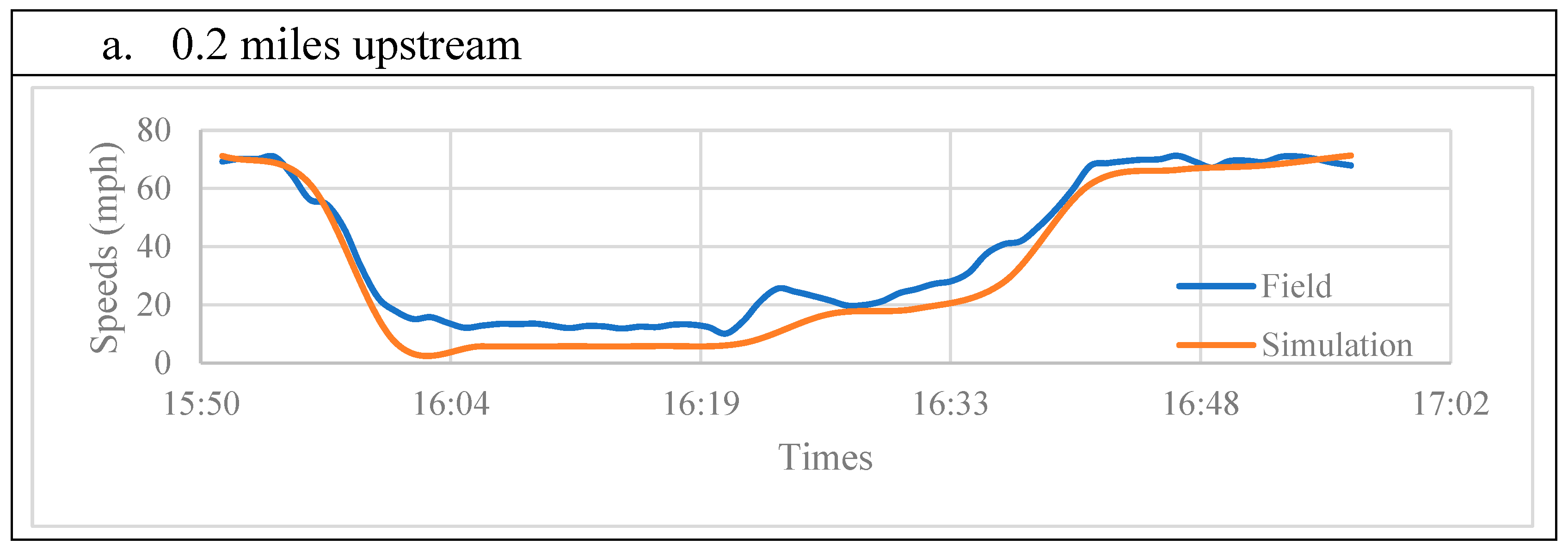
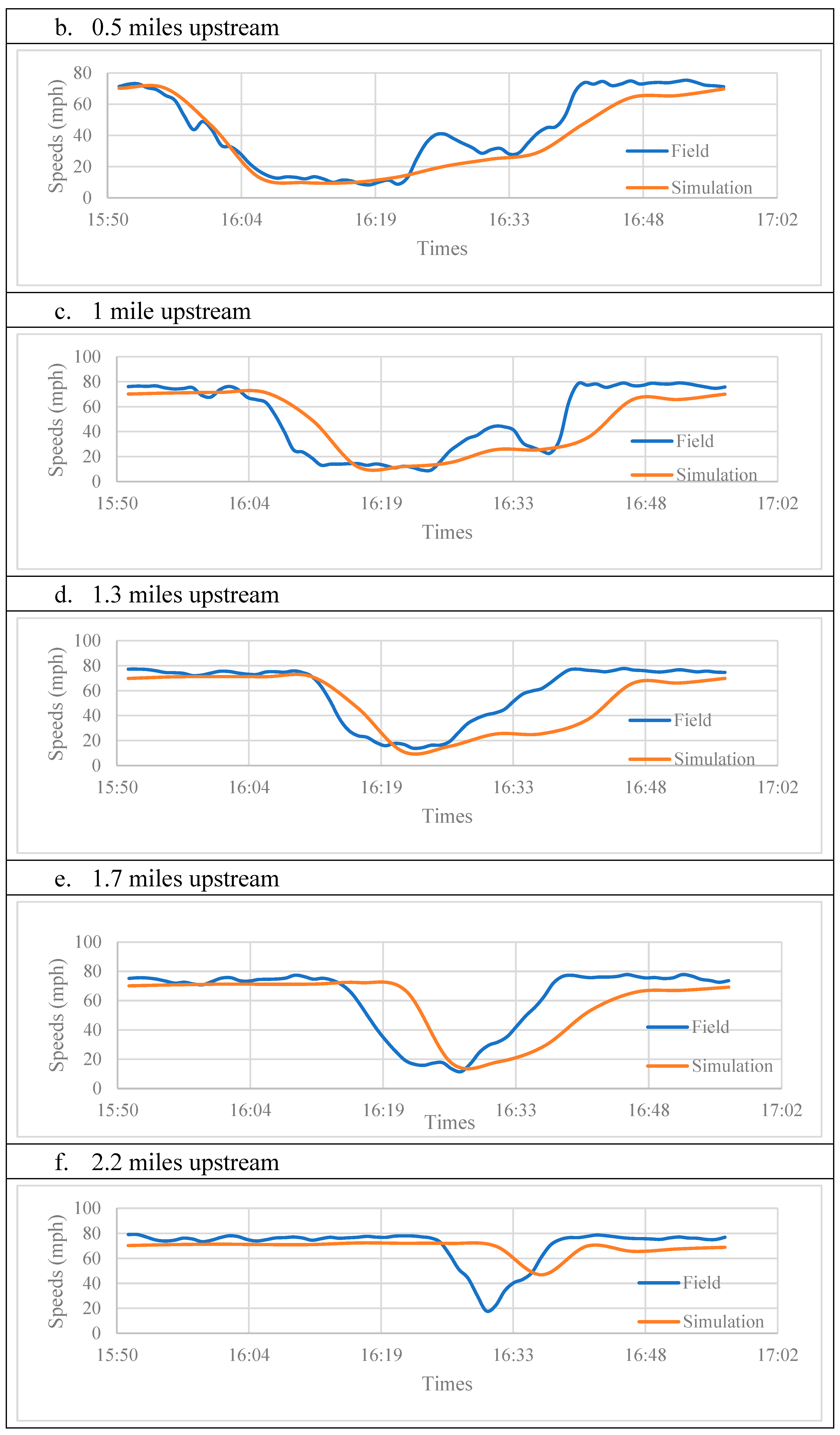
Furthermore, a comparison of speeds was conducted at each sensor location using the predetermined CC0 and CC1 values. Among the incidents analyzed, crash13 presented a more intricate scenario, encompassing data from six distinct sensors, as shown in Figure 1. This incident occurred on a four-lane freeway at 15:50, and one lane closed due to multiple car crashes. At 16:02, responders arrived and closed an additional lane to attend to the incident. By 16:21, all lanes were reopened. However, speed adjustments at the incident site were necessary because the Vissim calibration variables could not fully replicate the operational conditions at the incident site. Therefore, a speed restriction was applied to better represent real-world post-crash operations. The speed values at the incident site were set based on the average speed of open lanes nearest to the upstream sensor of the incident site when a queue was present due to lane closures. More detailed explanations can be found in Jeon [29].

The comparison of speed profiles between the field and simulation results defined the car-following model calibration variables for traditional vehicles. Ideally, the CAV car-following model should be calibrated using field data. However, incident-related CAV data were not available for 2021 crashes. Therefore, calibrated CC0 and CC1 parameters for traditional vehicles were incorporated into the “AV normal (CoEXist)” model in Vissim. Among three AV car-following models from Vissim—AV cautious (CoEXist), AV normal (CoEXist), and AV aggressive (CoEXist)—this study selected AV normal (CoEXist) for CAV operation. Thus, to better reflect realistic post-incident operations, the AV normal (CoEXist) was incorporated using calibrated CC0 and CC1 parameters. The calibration variables used in this study are summarized in

Table 4. Car-following model calibration variables.

Calibration Variable	Traditional Vehicles		CAV
	Default	Incident	AV Normal (CoEXist)	Incident
CC0 (Standstill distance)	4.92 ft.	15.0 ft.	4.92 ft.	15.0 ft.
CC1 (Gap time distance)	0.9 s	2.0 s	0.9 s	2.0 s
CC2 (‘Following’ distance oscillation)	13.12 ft.	13.12 ft.	0.00 ft.	0.00 ft.
CC3 (Threshold for entering ‘Following’)	−8.00	−8.00	−8.00	−8.00
CC4 (Negative speed difference)	−0.35	−0.35	−0.10	−0.10
CC5 (Positive speed difference)	0.35	0.35	0.10	0.10
CC6 (Distance dependency of oscillation)	0.00	0.00	0.00	0.00
CC7 (Oscillation acceleration)	0.82 ft/s2	0.82 ft/s2	0.33 ft/s2	0.33 ft/s2
CC8 (Acceleration from standstill)	11.48 ft/s2	11.48 ft/s2	11.48 ft/s2	11.48 ft/s2
CC9 (Acceleration at 50 mph)	4.92 ft/s2	4.92 ft/s2	4.92 ft/s2	4.92 ft/s2

☐: Modified calibration variables.

.

CAV may have different CC0 and CC1 compared to traditional vehicles, because of their capability to access incident information before they approach the incident site. Once post-incident traffic operation data for CAV becomes available, the calibration of CC0 and CC1 for CAV should be conducted to accurately reflect post-incident CAV operating conditions. Lastly, interactions between CAV and traditional vehicles were controlled by Vissim default settings, and it may not capture real-world post-incident traffic operating conditions.

6. Impact of CAV Market Penetration

In this section, Vissim was used to examine the effects of CAV market penetration levels on incident operation. Each condition had ten independent simulation runs using different random seeds from 43 to 52. Since each simulation run produced slightly different results, we report the aggregated average values.

This analysis was performed with the base volume condition as well as when the future volume was increased by 5%, 10%, and 15%. The CAV market penetration varied from 0% to 75%. The results showed that, as CAV market penetration increased, queue length decreased, travel time decreased, and average throughput during incident conditions increased.

6.1. Effects of Queue Length

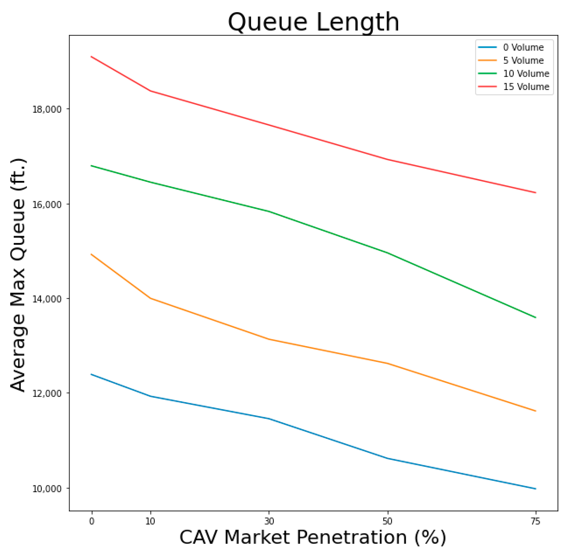
Queue length decreased as CAV market penetration increased, as shown in Figure 2. This trend was consistent across different traffic volumes increases.

Table 5. Queue length trends as CAV MP and volume changes.

CAV MP	Base Volume (0% Increase)		Future Volume Increased by
			5%		10%		15%
	Queue Length (ft.)	% Reduction	Queue Length (ft.)	% Reduction	Queue Length (ft.)	% Reduction	Queue Length (ft.)	% Reduction
0%	12,390		14,924		16,795		19,098
10%	11,928	4%	13,996	6%	16,449	2%	18,375	4%
30%	11,455	8%	13,132	12%	15,831	6%	17,657	8%
50%	10,617	14%	12,623	15%	14,957	11%	16,929	11%
75%	9975	19%	11,619	22%	13,592	19%	16,228	15%

☐: Base volume; ☐: 5% volume; ☐: 10% volume; ☐: 15% volume.

summarizes the changes in queue length as a function of both CAV market penetration for the base volume condition as well as when the future volume was increased by 5, 10, and 15 percent. As market penetration increased from 0 to 75%, the reductions in queue length were as high as 15–22%.

For base volume conditions, as the CAV MP increased from 0% to 75% the queue length was reduced by 0 to 19%. This signifies that a higher CAV MP leads to a more significant reduction in queue length during incident management. This trend was consistent when traffic volume increased by 5%, 10%, or 15%. As the volume increased, in general, the reduction in queue length was slightly lower, as expected.

6.2. Effects of Travel Time

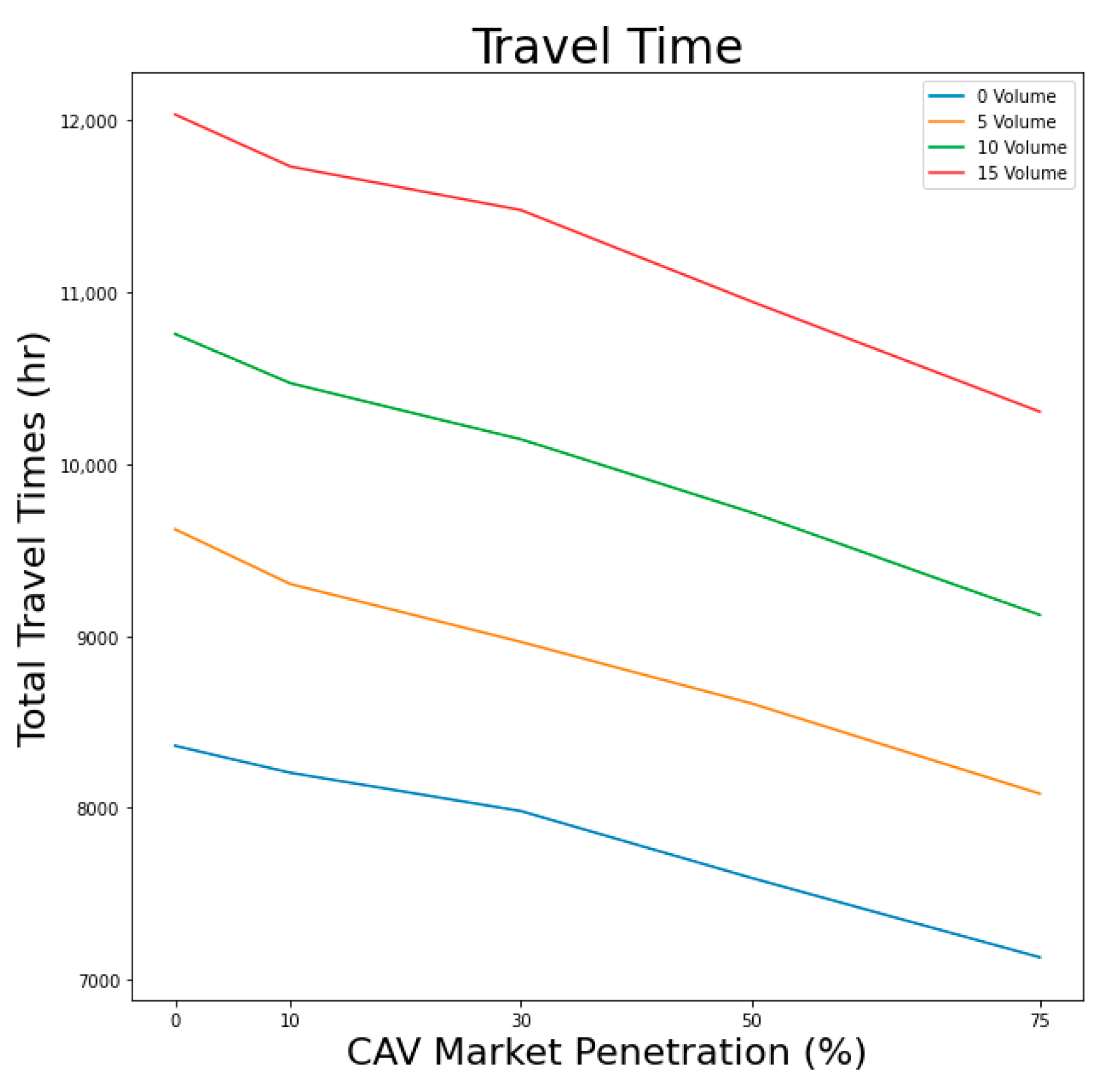
Similarly, travel time decreased as MP increased. Figure 3 shows the decreasing trends in travel time as CAV MP increased. For base volume conditions, as CAV MP increased from 0% to 75% the travel time reductions varied from 0 to 15%. This trend was consistent across different traffic volume increases.

Table 6. Travel time trends as CAV MP and volume changes.

CAV MP	Base Volume (0% Increase)		Future Volume Increased by
			5%		10%		15%
	Travel Time (h)	% Reduction	Travel Time (h)	% Reduction	Travel Time (h)	% Reduction	Travel Time (h)	% Reduction
0%	8362		9622		10,758		12,035
10%	8205	2%	9303	3%	10,472	3%	11,733	3%
30%	7982	5%	8966	7%	10,145	6%	11,479	5%
50%	7592	9%	8608	11%	9719	10%	10,947	9%
75%	7130	15%	8083	16%	9123	15%	10,306	14%

☐: Base volume; ☐: 5% volume; ☐: 10% volume; ☐: 15% volume.

summarizes the changes in travel time under different levels of CAV MP, offering valuable insights into the time-saving benefits of CAV during incidents. As the MP increased from 0 to 75%, the reductions in travel time reached 14−16%.

As the CAV MP increased from 0% to 75%, a consistent reduction in travel time was observed. This travel time decline highlights the potential for CAV to enhance the travel experience for both CAV users and traditional vehicle drivers during incidents, ultimately contributing to the efficiency of incident management. Similarly, when traffic volume increased by 5%, 10%, or 15%, travel time reduction was observed as 0% MP for each volume increase.

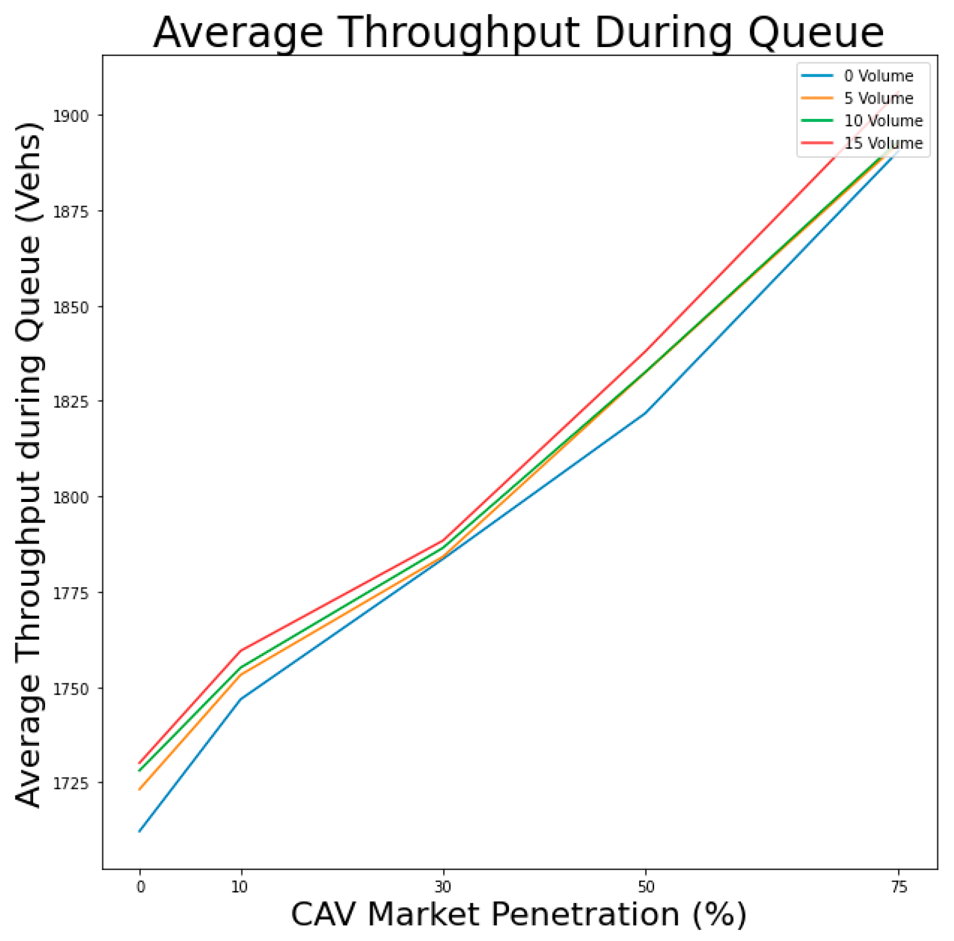
6.3. Effects of Throughput

The throughput was increased as CAV MP increased, as shown in Figure 4. This trend was consistent across different traffic volumes increases. As the MP increased from 0 to 75%, the throughput increased to as high as 10%.

Furthermore, the analysis revealed an interesting aspect of incident management: while there was an increase in average throughput during an incident as CAV MP increases, the average throughput during the incident remained relatively consistent across different traffic volume increases. This phenomenon could be attributed to incident-site conditions, which naturally reduced the number of open lanes and reduced speed near the incident site, leading to queue formation under all traffic volume conditions. Therefore, the average throughput during an incident tended to exhibit similar results, regardless of the traffic volume increase, as shown in

Table 7. Average throughput trends as CAV MP and volume changes.

CAV MP	Base Volume (0% Increase)		Future Volume Increased by
			5%		10%		15%
	Throughput (vehs)	% Increase	Throughput (vehs)	% Increase	Throughput (vehs)	% Increase	Throughput (vehs)	% Increase
0%	1712		1723		1728		1730
10%	1747	2%	1753	2%	1755	2%	1760	2%
30%	1784	4%	1784	4%	1787	3%	1788	3%
50%	1822	6%	1833	6%	1833	6%	1838	6%
75%	1891	10%	1892	10%	1893	10%	1906	10%

☐: Base volume; ☐: 5% volume; ☐: 10% volume; ☐: 15% volume.

.

This provided a comprehensive perspective on how incident site conditions and CAV MP together influence traffic flow during incidents. By understanding the impact of CAV MP on incident management, the management strategies can harness the full potential of CAV. These management strategies are developed to not only address incidents but also to optimize traffic flow, enhance safety, and ensure efficient management of adverse events on the road by minimizing turbulence.

7. Individual Benefit of Proposed Management Strategy

Each proposed management strategy was designed to reduce fluctuations near the incident site to enhance the safety of motorists and improve overall traffic operation. The effects of early merging of CAV into open lanes and CAV remaining in their lanes near the incident site were explored.

7.1. MS1-Longitudinal Control

MS1 signs served as essential elements in effective traffic management during incident operation, with their impact depending on both the displayed speed limit and its activation distances, and the compliance rate of traditional vehicles indicated the proportion of vehicles following the guided speed. The displayed speed will help upstream drivers to adapt early to changing traffic conditions to minimize turbulence from the activation distance. The detailed impacts of each aspect were explored in Jeon [29], while this paper specifically discusses the impact of the activation distance impact on travel time reduction.

As illustrated in Figure 5, the simulation results show that increasing the activation distance led to a travel time reduction across testing scenarios of 5, 10, and 15 miles. Nevertheless, it is important to note that extending the longitudinal control activation distance does not guarantee an indefinite enhancement in traffic operation. There exists an optimal activation distance where travel time can be minimized. Also, the optimal activation distance depends on factors such as arrival volume, CAV MP, and lane configurations.

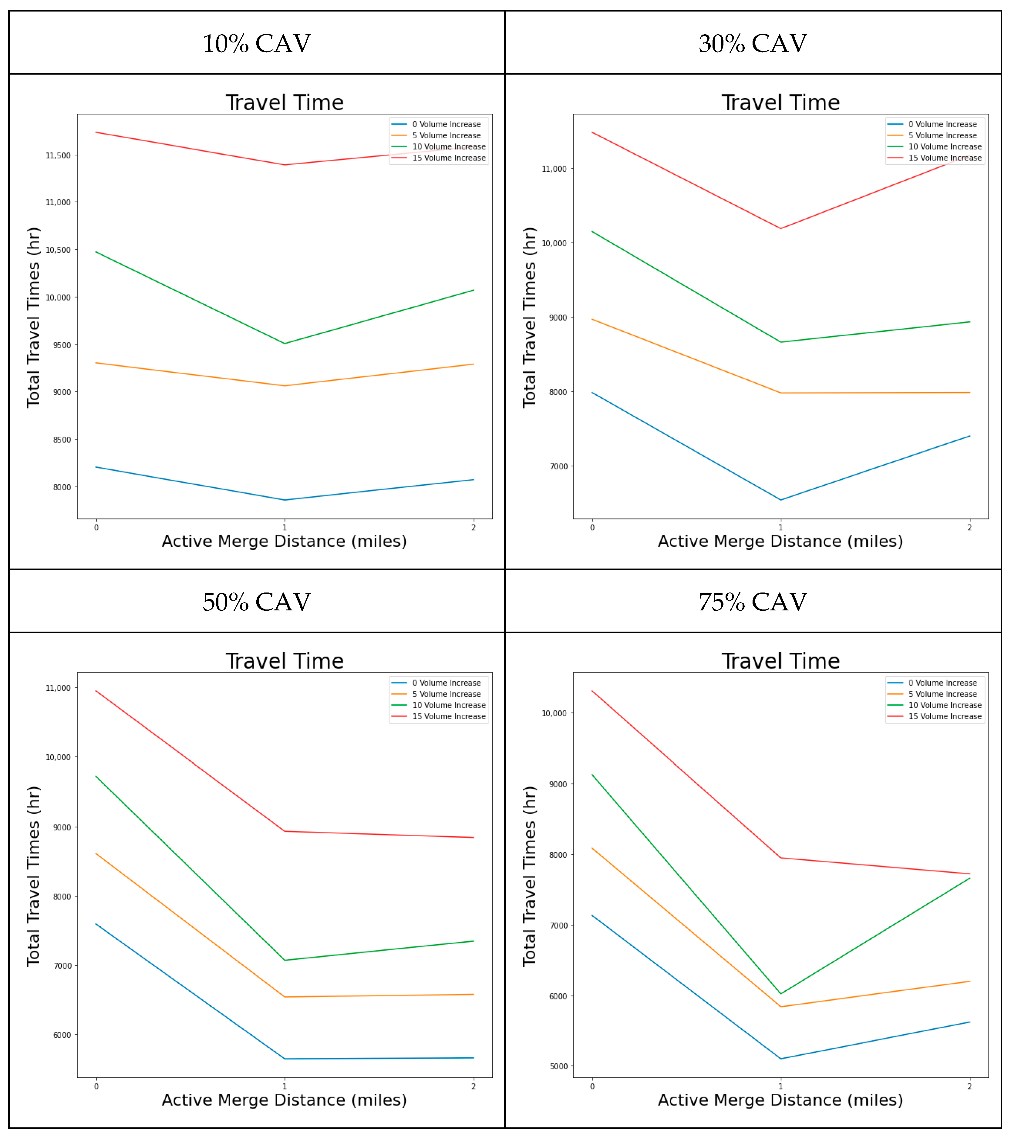
7.2. MS2-Directing CAV to Change Lanes Earlier

It is beneficial to CAV to travel on open lanes during incident operations, and Vissim simulation software provided a controlled environment to assess the potential advantages of this strategy. These simulation results offered a comprehensive view of how CAV interact with traditional vehicles during incident scenarios and their impact on traffic flow. By analyzing the travel time, the Vissim simulation results revealed the potential benefits of integrating CAV management strategies into incident management.

The Vissim simulations included scenarios where CAV changed lanes earlier at distances of 0, 1, and 2 miles upstream from the incident site. The results, as shown in Figure 6, revealed that CAV merging at 1 mile upstream exhibited the most favorable outcomes. MS2 encourages upstream CAV to merge early to minimize disruptions near the bottleneck by reducing last-minute lane changes. However, this strategy helps prevent abrupt lane changes; applying it too far upstream can lead to the underutilization of lane capacity where the queue effect is minimal or where the incident impact does not extend. Therefore, the optimal distance for implementing MS2 alone is approximately 1 mile upstream of the incident site. This effect is reflected in Figure 6, where the curve lowers at 1 mile, corresponding to the implementing location of MS2. This drop indicates reduced turbulence and improved traffic flow due to early merging.

7.3. MS3-Restricting CAV in Open Lanes from Lane Changes near Incidents

One of the important factors for traffic congestion near an incident site is last-minute lane changes by drivers. This can be alleviated by using CAV to remain in their open lanes near the incident site. Vissim software provides a controlled environment where the CAV were instructed to remain in their open lanes near the incident site.

The Vissim simulations showed that the benefit of CAV remaining in their open lanes was closely linked to CAV MP and input volume. For 10% CAV MP, travel time showed a slight increase, as depicted in Figure 7. As CAV MP increases gradually, a higher volume condition showed the benefit of reducing travel time. For example, 75% CAV MP showed all volume conditions except for the field volume condition showed a reduction in travel time, as shown in Figure 7.

8. Benefit of Implementing Combined Proposed Management Strategies

It was shown that individual MS could improve the operation depicted by reducing the travel time. There was potential when the proposed MS combined could further improve the operation.

Table 8. Benefits of combination of proposed MS on travel time.

	Field Volume Condition and 10% CAV MP			15% Volume Increase Condition and 50% CAV MP
	Travel Time (h)	Travel Time Reduction	Improvement	Travel Time (h)	Travel Time Reduction	Improvement
No CAV	8362			12,035
CAV with NO MS	8205	157	1.9%	10,947	1088	9.0%
MS1	7392	970	11.6%	9589	2446	20.3%
MS2	7858	504	6.0%	8928	3107	25.8%
MS3	8321	41	0.5%	9721	2314	19.2%
MS4	7075	1287	15.4%	7550	4485	37.3%
MS5	7499	863	10.3%	8348	3688	30.6%
MS6	8030	332	4.0%	8369	3666	30.5%
MS7	7216	1146	13.7%	7206	4829	40.1%

illustrates the effects of combining MS travel time with 10% and 50% CAV MP. For all conditions at 10% and 50% CAV MP, all of the proposed MS showed some improvement. However, it was not a full picture of benefits for implementing the proposed MS. When compared to CAV without MS, MS1 and MS2 showed a significant improvement in travel time as discussed in regard to individual benefit. However, for MS3 in 10% CAV MP, it showed slight deterioration compared to no MS as discussed in regard to individual benefit.

8.1. MS4

MS4 further reduced travel time compared to implementing MS1 or MS2 individually. For example, with a 10% CAV MP under field volume conditions showed travel time was substantially reduced by 1287 h (15.4%) compared to 11.6% for CAV with MS1 and 6.0% for CAV with MS2. This result underscored the effectiveness of implementing both management strategies concurrently to improve traffic flow and reduce congestion in incident operation.

8.2. MS5

The effectiveness of MS5 varied, depending on the combination of traffic volume and the CAV MP rate. For instance, at the base volume condition and 10% CAV MP, MS5 reduced travel time by only 10.3% while MS1 reduced it by 11.6%. However, when traffic volume was increased by 15% and CAV MP reached 50%, MS5 reduced travel time by 30.6%, surpassing the 20.3% reduction achieved by MS1.

8.3. MS6

Similar to MS5, the effectiveness of MS6 also depended on the combination of traffic volume and CAV MP. For instance, at the base volume condition and 10% CAV MP, MS6 reduced travel time by only 4.0%, while MS2 reduced it by 6.0%. However, when traffic volume was increased by 15% and CAV MP reached 50%, MS6 reduced travel time by 30.5% which is greater than 25.8% for MS2.

8.4. MS7

More restricted MS, such as MS7, did not always yield more efficient incident management than a less restricted MS for all traffic conditions. For example, at the base volume condition and 10% CAV MP, MS7 reduced travel time only by 13.7% compared to MS4, which reduced it by 15.4%. However, when traffic volume was increased by 15% and CAV MP became 50%, MS7 yielded the largest travel time reduction of 40.1% compared to 37.3% for MS4.

9. Conclusions and Recommendations

This study first determined the operational impacts of CAV on freeway incidents management (using Vissim simulation software) when no traffic management strategy was implemented. As CAV MP increased, queue length and travel time decreased. For instance, with a 10% CAV MP, the queue length was reduced by 2–6%, and travel time was reduced by 2–3%, depending on the traffic volume.

Then it determined the effects of seven proposed MS (three individual strategies and four combined strategies). MS1 improved travel time by controlling the arrival volume and arrival speed. Increasing the activation distance of longitudinal control resulted in travel time reduction across testing scenarios of 5, 10, and 15 miles. MS1 reduced travel time by 11.6% compared to 1.9% for no MS at 10% CAV MP. MS2 reduced the turbulence near the incident bottleneck, and it was most effective when applied at 1 mile upstream of the incident site. It reduced travel time by 6.0% compared to 1.9% for no MS at 10% CAV MP. In MS3, the beneficial effects (travel time reduction) became more pronounced as CAV MP increased. At 50% CAV MP, the travel time reduction was 19.2% compared to 9.0% with no MS.

Some of the combined strategies (MS 4 to 7) were more effective than other strategies. For example, MS4 with 10% MP reduced travel time by 15.4% compared to 11.6% for MS1 and 1.9% for no MS, making MS4 eight times more effective than no MS. MS4 outperformed MS5 and MS6 in reducing travel time (15.4% compared to 10.3% and 4.0%). MS4 was even more effective than MS7 at 10% CAV MP. However, at 50% CAV MP, MS7 reduced travel time by 40.1% compared to 37.3% reduction achieved by MS4. Therefore, the incident management strategies should be selected considering the CAV MP and traffic volume conditions, and the more restricted traffic management strategy may not yield the most efficient operation for all conditions. Findings from the simulation runs showed the significance of combining the management strategies with CAV.

Management Strategy Guidance for Local Authorities

The findings of this study provide valuable insights for local transportation agencies and policymakers in enhancing freeway incident management in a CAV environment. To successfully implement the proposed MS, local agencies should consider the following key aspects:

• Infrastructure Readiness: Local authorities should ensure that roadway infrastructure and traffic management systems are equipped to support traditional vehicles and CAV operations. This includes dedicated communication networks for CAV, VSL, and dynamic message signs (DMS) to inform drivers and improve traffic operation;
• Strategic Policy Implementation: The effectiveness of incident management strategies depends on CAV MP and prevailing traffic conditions. Policymakers should develop adaptive incident management policies that adjust strategies based on real-time CAV MP, traffic demand, and the severity of incident-induced congestion;
• Selection of Effective Management Strategies: Based on this study, policymakers should prioritize MS based on CAV MP and travel demand. For example, MS4 is most effective for field volume and the 10% CAV MP condition. On the other hand, MS7 is most for a 15% volume increase and 50% CAV MP condition. Thus, policymakers should select MS dynamically based on prevailing traffic and incident conditions, rather than applying a single fixed strategy;
• Applicability of Management Strategies: The proposed MS are tailored to specific incident and traffic conditions observed in this study. For other incident scenarios, additional studies may be needed to identify the most effective strategy based on the prevailing conditions.

By integrating these policy measures, transportation agencies can maximize the benefit of CAV technologies to improve post-incident traffic operation by mitigating congestion and improving roadway safety.

References

- Schrank, D.; Albert, L.; Jha, K.; Eisele, B. 2023 Urban Mobility Report; Texas A&M Transportation Institute, Mobility Division: Bryan, TX, USA, 2023. [Google Scholar]
- Cambridge Systematics. Traffic Congestion and Reliability: Trends and Advanced Strategies for Congestion Mitigation; No. FHWA-HOP-05-064; Federal Highway Administration: Washington, DC, USA, 2005. [Google Scholar]
- SAE On-Road Automated Vehicle Standards Committee. Taxonomy and definitions for terms related to on-road motor vehicle automated driving systems. SAE Stand. J 2014, 3016, 1. [Google Scholar]
- Raub, R.A. Occurrence of secondary crashes on urban arterial roadways. Transp. Res. Rec. 1997, 1581, 53–58. [Google Scholar] [CrossRef]
- Moore, J.E.; Giuliano, G.; Cho, S. Secondary accident rates on Los Angeles freeways. J. Transp. Eng. 2004, 130, 280–285. [Google Scholar] [CrossRef]
- Vlahogianni, E.I.; Karlaftis, M.G.; Golias, J.C.; Halkias, B.M. Freeway operations, spatiotemporal-incident characteristics, and secondary-crash occurrence. Transp. Res. Rec. 2010, 2178, 1–9. [Google Scholar] [CrossRef]
- Chung, Y. Identifying primary and secondary crashes from spatiotemporal crash impact analysis. Transp. Res. Rec. 2013, 2386, 62–71. [Google Scholar] [CrossRef]
- Xu, C.; Liu, P.; Yang, B.; Wang, W. Real-time estimation of secondary crash likelihood on freeways using high-resolution loop detector data. Transp. Res. Part C Emerg. Technol. 2016, 71, 406–418. [Google Scholar] [CrossRef]
- Ghiasi, A.; Li, X.; Ma, J. A mixed traffic speed harmonization model with connected autonomous vehicles. Transp. Res. Part C Emerg. Technol. 2019, 104, 210–233. [Google Scholar] [CrossRef]
- Abdulsattar, H.; Mostafizi, A.; Siam, M.R.; Wang, H. Measuring the impacts of connected vehicles on travel time reliability in a work zone environment: An agent-based approach. J. Intell. Transp. Syst. 2020, 24, 421–436. [Google Scholar] [CrossRef]
- Haque, M.S.; Rilett, L.R.; Zhao, L. Impact of platooning connected and automated heavy vehicles on interstate freeway work zone operations. J. Transp. Eng. Part A Syst. 2023, 149, 04022160. [Google Scholar] [CrossRef]
- Singh, M.K.; Formosa, N.; Man, C.K.; Morton, C.; Masera, C.B.; Quddus, M. Assessing temporary traffic management measures on a motorway: Lane closures vs narrow lanes for connected and autonomous vehicles in roadworks. IET Intell. Transp. Syst. 2024, 18, 1210–1226. [Google Scholar] [CrossRef]
- Wang, L.; Zhong, H.; Ma, W.; Abdel-Aty, M.; Park, J. How many crashes can connected vehicle and automated vehicle technologies prevent: A meta-analysis. Accid. Anal. Prev. 2020, 136, 105299. [Google Scholar] [CrossRef]
- Boggs, A.M.; Wali, B.; Khattak, A.J. Exploratory analysis of automated vehicle crashes in California: A text analytics & hierarchical Bayesian heterogeneity-based approach. Accid. Anal. Prev. 2020, 135, 105354. [Google Scholar]
- Scanlon, J.M.; Kusano, K.D.; Daniel, T.; Alderson, C.; Ogle, A.; Victor, T. Waymo simulated driving behavior in reconstructed fatal crashes within an autonomous vehicle operating domain. Accid. Anal. Prev. 2021, 163, 106454. [Google Scholar] [CrossRef] [PubMed]
- Makahleh, H.Y.; Badrawi, H.A.; Abdelfatah, A. Assessing the Impacts of Autonomous Vehicles for Freeway Safety. In Proceedings of the 10th World Congress on New Technologies (NewTech’24), Barcelona, Spain, 25–27 August 2024; pp. 25–27. [Google Scholar]
- Smith, B.L.; Qin, L.; Venkatanarayana, R. Characterization of freeway capacity reduction resulting from traffic accidents. J. Transp. Eng. 2003, 129, 362–368. [Google Scholar] [CrossRef]
- Hadi, M.; Sinha, P.; Wang, A. Modeling reductions in freeway capacity due to incidents in microscopic simulation models. Transp. Res. Rec. 2007, 1999, 62–68. [Google Scholar] [CrossRef]
- Addison, J.; Aghdashi, S.; Rouphail, N.M. Evaluating the effect of incidents on freeway facilities and updating the incident capacity adjustments for HCM. Transp. Res. Rec. 2021, 2675, 224–234. [Google Scholar] [CrossRef]
- Smulders, S. Control of freeway traffic flow by variable speed signs. Transp. Res. Part B Methodol. 1990, 24, 111–132. [Google Scholar] [CrossRef]
- Hegyi, A.; De Schutter, B.; Heelendoorn, J. MPC-based optimal coordination of variable speed limits to suppress shock waves in freeway traffic. In Proceedings of the 2003 American Control Conference, Denver, CO, USA, 4–6 June 2003; Volume 5, pp. 4083–4088. [Google Scholar]
- Popov, A.; Hegyi, A.; Babuška, R.; Werner, H. Distributed controller design approach to dynamic speed limit control against shockwaves on freeways. Transp. Res. Rec. 2008, 2086, 93–99. [Google Scholar] [CrossRef]
- Waller, S.T.; Ng, M.; Ferguson, E.; Nezamuddin, N.; Sun, D. Speed Harmonization and Peak-Period Shoulder Use to Manage Urban Freeway Congestion; No. FHWA/TX-10/0-5913-1; University of Texas at Austin, Center for Transportation Research: Austin, TX, USA, 2009. [Google Scholar]
- McMurtry, T.; Saito, M.; Riffkin, M.; Heath, S. Variable speed limits signs: Effects on speed and speed variation in work zones. In Proceedings of the 88th Annual Meeting of the Transportation Research Board, Washington, DC, USA, 11–15 January 2009. [Google Scholar]
- Hadiuzzaman, M.; Qiu, T.Z.; Lu, X.Y. Variable speed limit control design for relieving congestion caused by active bottlenecks. J. Transp. Eng. 2013, 139, 358–370. [Google Scholar] [CrossRef]
- Ramezani, H.; Benekohal, R. Optimized speed harmonization with connected vehicles for work zones. In Proceedings of the 2015 IEEE 18th International Conference on Intelligent Transportation Systems, Gran Canaria, Spain, 15–18 September 2015; pp. 1081–1086. [Google Scholar]
- Ma, W.; Chen, B.; Yu, C.; Qi, X. Trajectory planning for connected and autonomous vehicles at freeway work zones under mixed traffic environment. Transp. Res. Rec. 2022, 2676, 207–219. [Google Scholar] [CrossRef]
- Ko, B.; Ryu, S.; Park, B.B.; Son, S.H. Speed harmonisation and merge control using connected automated vehicles on a highway lane closure: A reinforcement learning approach. IET Intell. Transp. Syst. 2020, 14, 947–957. [Google Scholar] [CrossRef]
- Jeon, H.J. Optimal Highway Incident Operation with Active Traffic Management and Connected Automated Vehicle. Ph.D. Dissertation, University of Illinois at Urbana-Champaign, Champaign, IL, USA, 2023. [Google Scholar]
- Kan, X.D.; Ramezani, H.; Benekohal, R.F. Calibration of VISSIM for Freeway Work Zones with Time-Varying Capacity. In Proceedings of the 93rd Annual Meeting of the Transportation Research Board, Washington, DC, USA, 12–16 January 2014; p. 14-3615. [Google Scholar]