Network Screening on Low-Volume Roads Using Risk Factors

Abstract

This paper proposes a new method for network screening on rural low-volume roads. These roads are important as they provide critical access to agricultural land and tourist attractions. Most low-volume roads belong to the lowest functional class (local rural roads) and thus are built to lower design standards. Conventional hot spot network screening techniques may not be appropriate for low-volume roads due to the sporadic nature of crashes occurring on these roads. Conversely, sophisticated network screening approaches require extensive roadway and traffic data that are often unavailable to local agencies due to a lack of resources, and/or a lack of technical expertise. This research attempts to address these obstacles to low-volume road network screening which aims to identify candidate sites for safety improvements. The research used an extensive low-volume road sample from the state of Oregon and Empirical Bayes expected number of crashes in developing the proposed models for network screening. The proposed models do not require exact measurements of roadway geometric features as all geometric variables were classified into categories that are easy to compile by local agencies. Further, the method could be used with and without traffic data, without compromising the effectiveness of the network screening process.

1. Introduction

Low-volume roads (LVRs) constitute a large proportion of the rural roadway network, providing critical access to remote rural areas and tourist attractions. These roads are characterized by low traffic volumes, lower functional classifications, and many of them are built to lower standards (e.g., narrow lanes and shoulders, non-forgiving roadsides, etc.). Moreover, average travel speeds on these roads are generally high (like other rural roadways), which largely explains the higher crash fatality rates on these roads compared to those in urban areas [1]. In the United States, as well as in most other developed countries, safety is managed on the highway network using highway safety improvement programs. These programs, which aim to reduce the number and severity of crashes on a road network, are ongoing programs funded by the government and are usually managed by state transportation agencies. A critical step in these programs is network screening, where candidate sites for safety improvement are identified and ranked according to priority throughout the network for further consideration and analysis. A common rule used by most safety improvement programs is to maximize safety benefits at the selected sites to ensure optimum use of safety funds.

Historically, the most common approach to network screening has been the use of crash history, i.e., crash frequencies, severities, and/or rates, to identify sites for safety improvements. While this approach may work reasonably well for networks with high traffic exposure (e.g., urban areas and major rural routes), it may prove unsuitable for low-volume roads. Specifically, due to low traffic volumes, only a limited number of crashes occur during the analysis period, which tend to be scattered sporadically throughout the network. Therefore, it is unlikely that a site would consistently show a significant number of crashes to be ranked high on a ranking list using crash frequencies. On the other hand, many LVR sites with very low crash frequencies may still rank high when crash and/or fatality rates are used in screening the network. Sites selected using the latter approach may not necessarily result in maximizing safety benefits at the network level. Therefore, a more sophisticated network screening approach, which considers factors other than crash history, such as roadway and traffic characteristics, is more effective in screening LVR networks. However, these methods (e.g., Empirical Bayes) often require detailed roadway, traffic, and crash data and use advanced statistical tools, which may present implementation challenges. Specifically, many LVRs are owned and operated by local agencies (townships, counties, tribal governments, etc.) that usually lack the adequate resources and technical staff to adopt such sophisticated methods. Therefore, an ideal network screening method for LVRs would require few resources while being effective in identifying sites associated with a high potential for crash reduction.

In this study, LVRs are defined as rural roads with annual average daily traffic equal to or less than 1000 vehicles per day (vpd). This definition is consistent with that used in a few other studies found in the literature [2,3].

2. Background

Network screening is a well-researched area, and several network screening methods have been developed over time. However, only limited information is available regarding network screening for rural two-lane roadways, and even less for rural low-volume roads. Only a couple of methods have been implemented in practice, while a few other methods have been proposed in the literature without necessarily being implemented by highway agencies.

2.1. Network Screening Methods Implemented in Practice

As is to be expected, methods that are reported as being used by highway agencies on local rural roads are generally simple and require a minimal amount of information for implementation. One such method utilizes the Federal Highway Administration (FHWA) Systemic Project Selection tool [4]. Risk factors are identified based on the relationship between roadway variables and crash occurrence. Locations having one or more of these risk factors are scored with a “1” or an asterisk. After reviewing the locations, the risk factors are reassessed for their usefulness in the identification of safety improvement locations across the whole network. Any risk factor that is present at every location of the network is discarded. Finally, the locations are ranked based on the presence of risk factors. Sites with a higher number of risk factors indicate higher crash risk and therefore have higher priority. A few states and counties have reported the use of this tool. The “star” approach [5,6] in ranking sites for safety improvement consideration follows the same concept. If a risk factor of interest is present at a site, then a star is assigned. The higher the number of stars, the higher the risk at a site and the higher priority the site receives.

2.2. Methods Proposed in the Literature

Several studies proposed network screening methods on rural roads with no re-ported implementation or adoption by highway agencies. Most of these methods use the relationship between risk factors or surrogate safety measures and crash numbers to predict the future number of crashes or level of risk throughout the network. Traffic or roadway characteristics that have a strong correlation with crash occurrence are known as risk factors and may be used as surrogate safety measures. A study [7] of rural roads in Wyoming has developed crash prediction models using negative binomial regression (NBR) and the Poisson regression method. The models used crash rate, traffic volume, and speed and found that the high crash rates have a strong correlation with high traffic volumes and high speeds. The study also found that the NBR models had a better fit for the data. Another study [8] developed a full Bayes multivariate crash prediction model for rural two-lane roads in Pennsylvania. This study used traffic volume and segment length to predict crash frequencies. Al-Kaisy et al. [9] developed a risk index to identify at-risk locations for state-owned LVRs in Oregon. This method used three elements; namely, geometric features, crash history, and traffic exposure. Suitable weights were assigned to each element and then the elements along with their weights were used to calculate a risk index for a site. The same author also proposed a scoring-based network screening approach [10] using relationships between crash occurrences and risk factors in Montana. A study from New Zealand [11] used speed to identify at-risk horizontal curves on rural highways. The study calculated the operating speeds on curves using an Austroads (Australian transportation agency) operating speed prediction model. Then, the operating speeds were compared with the radius of the horizontal curves to assess the design limitation of the curves.

The more sophisticated Empirical Bayes (EB) method [12] was also reported as being evaluated on rural local roads. One study [13] used simulated data for low-volume two-lane roads to measure the performance of different screening methods. The study concluded that the EB method outperformed other methods considered in this investigation. Superior performance of the EB method for LVRs was also reported by a US-based study [14] using empirical crash data. In addition to LVRs, the EB method was reported by multiple studies [15,16,17] to have superior performance for network screening on urban roads as well. Another European study [18] used the difference between observed and predicted crashes per unit length of road to find the accident potential for a site. Sites with positive accident potentials were considered as at-risk sites. Lastly, an Ethiopian study [19] used the difference between the EB expected crash numbers and the predicted crash numbers to identify and rank at-risk sites on a rural highway. The superior performance of the EB method is expected since the method uses traffic, geometric, and historical crashes to predict future crashes. However, the use of all these variables and the complex structure by the EB method require extensive crash, roadway, and traffic databases and well-trained personnel for implementation. Given these requirements, small and local agencies (e.g., counties, townships, and tribal governments) would find it impractical to adopt the EB method for identifying safety improvement sites.

3. Motivation

The sporadic nature of the crash occurrences on LVRs makes the conventional network screening methods using crash history unsuitable for use on rural local road networks. Further, the couple of network screening methods that have been reported in the literature as being implemented by highway agencies are too simplistic to accurately and effectively identify sites deserving more consideration in terms of safety treatments. At the other end, the more sophisticated network screening methods (e.g., EB and EB-related methods) require extensive crash, roadway, and traffic data along with technical expertise that are typically unavailable or inaccessible for local agencies such as towns, counties, and tribal governments. Therefore, the main objective of the current study was to develop a practical and effective method for network screening on rural LVRs which requires a minimal amount of information and technical expertise for implementation by local agencies.

4. Study Data

State-owned LVR data from Oregon was used to develop this new method. The study sample consisted of around 850 miles of low-volume roads from different regions in the state. The Oregon Department of Transportation (ODOT) online databases and video logs were used to identify and compile traffic, geometric, and crash data. Data were collected for roadway sections that are 0.05 miles in length (analysis units). While the 0.05-mile length is a relatively short distance, it was deemed important to make sure changes in roadway and roadside characteristics are captured with reasonable accuracy.

While both highway segments and intersections are integral parts of roadway networks, their characteristics, risk factors, and crash patterns are different. Expectedly, for rural low-volume roads, the number of intersections in the roadway network is notably smaller, as most roadways are in less developed areas outside of major towns and cities. This research focused solely on roadway segments, with the understanding that a similar approach could be applied to rural intersections using different variables. All the segments were for two-lane paved rural roads with a posted speed limit of 55 mph.

Traffic volume and roadway data were collected for each of the 0.05-mile sections. Roadway data included information about lane width, shoulder width, horizontal curves, spiral curves, vertical grade, driveway density, side slope, and roadside fixed objects. The Oregon DOT video logs were used to collect driveway density, side-slope rating, and fixed-object rating data. Fixed-object and side-slope data were collected categorically as it was not possible to collect their exact information from video logs. Crash data from 2004 to 2013 were also collected for each of the 0.05-mile sections.

5. Methodology

As stated previously, the proposed new method should satisfy two requirements: (1) the method is effective in identifying sites that are more deserving of safety treatments, and (2) the method requires little information and technical skills that are accessible to local agencies. To satisfy these requirements, the method developed in this research incorporated the following two features:

• The EB expected number of total crashes was selected as a basis for network screening in the proposed method. This is to ensure effective network screening given the favorable performance of the EB method for LVRs [13,14]. In addition, multiple studies [15,16,17] have also reported favorable performance of the EB method over other methods used for network screening.
• The proposed method employs classified variables that can easily be compiled by local agencies using staff with limited technical skills. The risk factors were selected based on the findings from a previous study [9], that identified different risk factors for Oregon LVRs.

5.1. Overview of the EB Method

The EB method employs the predicted number of crashes and the observed number of crashes to estimate the expected number of crashes at a specific site. This estimation is developed using Equation (1):

$$N_{expected}={w\times N}_{predicted}+\left(1-w\right)\times N_{observed}$$

(1)

This equation assigns different weights ($w$ in Equation (1)) to the predicted and observed numbers of crashes in estimating the expected number of crashes. The predicted number of crashes is found using a predictive mathematical model, also known as safety performance function (SPF). While many SPFs are proposed in the literature for various types of highway facilities, this study used the SPF proposed by the Highway Safety Manual (HSM) for rural two-lane highways [12], which is calibrated for the state of Oregon [20]. The predictive HSM method predicts the number of crashes at a specific site in a two-step process. First, the method utilizes the SPF mathematical model in predicting the number of crashes under base conditions (e.g., for two-lane highway segments, inputs are the AADT and segment length). Then, the method accounts for roadway and roadside characteristics (sometimes referred to as risk factors) that deviate from the base conditions using crash modification factors (CMFs). The observed number of crashes is the number of reported crashes at the specific site for the same analysis period. The weight ($w$) of a segment is calculated using Equation (2).

$$w=\frac{1}{(1+k\times N_{predicted})}$$

(2)

The $k$ in Equation (2) is the over-dispersion parameter associated with the SPF and the formula for calculating it is provided in the HSM as well [12]. The formula for calculating $k$ is shown in Equation (3).

$$k=\frac{0.236}{\mathit{\text{Segment}} \mathit{\text{Length}} (=0.05 \mathrm{m}\mathrm{i}\mathrm{l}\mathrm{e})}$$

(3)

5.2. Classification of Roadway Variables

More sophisticated network screening methods use exact values for various roadway characteristics (sometimes referred to as risk factors) when applying the screening procedure. While the use of exact values may improve the accuracy of the screening process, it requires access to extensive databases or on-site detailed measurements which are typically beyond the resources available for small local agencies. Hence, implementing such sophisticated methods might not be feasible for most local agencies. One possible solution to this problem is to use a classified format instead of the exact values for roadway characteristics that can easily be acquired by local agencies. This approach would classify any roadway variable or risk factor (e.g., lane width) into a limited number of categories for use in the prospective screening procedures. Therefore, the issue that had to be addressed by this research is how to set the cut-off values between the classes or categories of classified variables. To avoid any subjectivity in the process of setting cut-off values, it was decided to use the classification and regression tree (CART) data mining technique. CART analysis classifies an independent variable based on the effect it has on a dependent variable. It can be used to determine the relative importance of different variables for identifying homogeneous groups within the dataset. The analysis recursively partitions observations in a matched dataset, consisting of a categorical or continuous dependent (response) variable and one or more independent (explanatory) variables, into progressively smaller groups [21]. Each partition is a binary split. During each recursion, splits for each independent (explanatory) variable are examined and the split that maximizes the homogeneity of the two resulting groups with respect to the dependent (response) variable is chosen. In short, the CART algorithm divides the data into different groups, where data points within a group are similar to each other, while the datapoints in different groups are different from each other. In this study, the dependent variable was the expected crash numbers (from the HSM EB method), and the independent variables were the roadway characteristics or risk factors. When the CART analysis failed to provide suitable cut-off values for classifying the risk factors, the identified trends of crash occurrences with different risk factors were used for determining suitable cut-off values for classification.

The main purpose of classifying the data was to ease the efforts of data collection. However, collecting exact data for a couple of variables is comparatively easier than others and therefore these variables were intentionally not classified. The first variable is the driveway density. The driveway density for a segment can easily be obtained from updated maps (for example Google Earth or Google Maps) of the segments and, as such, were not classified using CART. The second variable is traffic volume as AADT has increasingly been used by highway agencies for many purposes and, as such, highway agencies usually measure or estimate AADT for most of their roadway networks. Further, it was deemed impractical to classify volume data due to the difficulty of selecting traffic volume classes without prior knowledge about traffic volume. The side-slope and roadside fixed-object data were excluded from the CART analysis because these variables were already collected in a classified format using the roadway video logs accessible through the Oregon DOT website.

5.3. Development of Regression Model

After classifying roadway (or risk) factors, models were developed to predict the level of risk (or safety) of roadway segments using the study sample. Two models were developed for this purpose. The response (dependent) variable in both models was the EB expected number of crashes, which is a function of the HSM predicted number of crashes and the observed number of crashes. The explanatory (independent) variables included classified roadway factors and traffic exposure (AADT) for the first model and only classified roadway factors for the second model. This was carried out so that the network screening could be performed with or without the use of AADT data, as many local agencies lack the resources to acquire traffic volume data on their respective networks.

6. Study Results

This section presents the results of the different analyses that were carried out to develop the new network screening method. The proposed method is in the form of regression models that use roadway characteristics and traffic exposure to assess the level of risk or safety for roadway segments.

6.1. Level of Risk

The proposed models use the EB expected number of crashes as an indicator of the level of risk associated with any roadway segment that is part of the network. This measure incorporates roadway physical characteristics, traffic exposure, and observed crashes in assessing the level of risk, and thus is more comprehensive than using either the HSM predicted number of crashes alone or the observed number of crashes alone. This measure serves as the response or dependent variable in the proposed models.

6.2. Model Variables

This section discusses the explanatory or independent variables used in developing network screening predictive models.

Table 1. Explanatory variables of the proposed models.

Risk Factors	Approximate Ranges of Variables	Categories	Terms	Statistics/Frequencies
Lane Width (LW)	LW < 11 ft	1	Narrower	Frequency: 1964
	LW ≥ 11 ft	2	Wider	Frequency: 14,550
Shoulder Width (SW)	SW < 2 ft	1	Narrower	Frequency: 5508
	SW ≥ 2 ft	2	Wider	Frequency: 11,006
Degree of Horizontal Curvature (DC)	DC = 0°	0	Straight	Frequency: 10,038
	DC < 9°	1	Mild	Frequency: 5322
	9° ≤ DC < 28°	2	Moderate	Frequency: 615
	DC ≥ 28°	3	Sharp	Frequency: 539
Grade (G)	G < 4%	0	Mild	Frequency: 12,593
	G ≥ 4%	1	Steep	Frequency: 3921
Driveway Density (DD) (driveways per mile)	Exact Number			Minimum: 0 First Quartile: 0 Median: 0 Mean: 4.479 Third Quartile: 0 Maximum: 100
Side Slope (SS)	Steep	1	Steep	Frequency: 3363
	Moderate	2	Moderate	Frequency: 10,871
	Flat	3	Flat	Frequency: 2280
Fixed Objects (FO)	Many	1	Many	Frequency: 10,700
	Some	2	Some	Frequency: 4458
	Few	3	Few	Frequency: 1356
Volume (V)	Exact Volume			Minimum: 60 First Quartile: 260 Median: 430 Mean: 496.5 Third Quartile: 620 Maximum: 2500
Dependent Variable: EB Expected Number of Crashes				Minimum: 0.0083 First Quartile: 0.0376 Median: 0.0561 Mean: 0.0994 Third Quartile: 0.0821 Maximum: 5.1193

shows the explanatory variables for the proposed models. Some of the cut-offs were rounded to the nearest whole number for practical purposes.

As shown in this table, traffic volume (AADT) and driveway density use exact values. The AADT is usually measured or estimated for highway segments as it is used by highway agencies for different purposes. Classifying traffic volume was deemed inappropriate for the difficulty in selecting the appropriate class without a prior knowledge of traffic volume. It was also decided to use the exact number of driveways per mile as this information is easily accessible using aerial photography available through web mapping applications such as Google Maps. All other variables shown in this table are in a classified format. Roadside variables, side slope, and fixed objects were already compiled in a classified format when the information was extracted from video logs, and therefore no classification was needed. The CART analysis discussed earlier was used to classify the other variables; namely, lane width, shoulder width, degree of curvature, and grade. The open-source statistical software R (https://www.r-project.org/) was used for running the CART analyses.

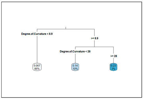
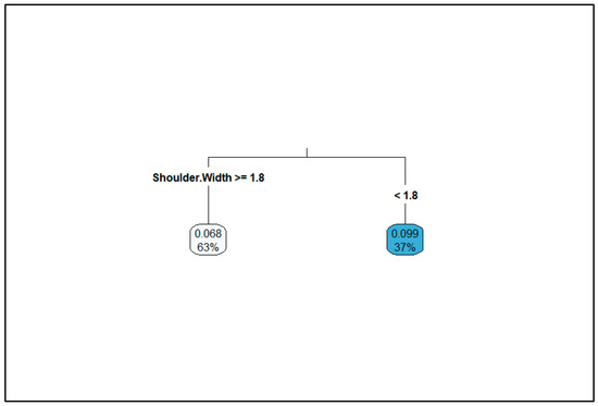
The CART results for the degree of curvature are shown in Figure 1. It can be seen from the output that 86 percent of the data comprises segments that have a degree of curvature less than 8.9 degrees. This 86 percent corresponds to the lowest average expected number of crashes of 0.067. The next branch shows that 10 percent of the data comprises segments with degrees of curvature equal to or greater than 8.9 degrees but less than 28 degrees. This group corresponds to the average expected number of crashes of 0.14. The third branch of the output shows segments with degrees of curvature equal to or greater than 28 degrees. This group constitutes three percent of the data and corresponds to an average expected number of crashes of 0.86. Based on this output, four classes were selected for horizontal curvature: straight segments with degrees of curvature of zero, mild curves with degree of curvature greater than 0 but less than 8.9 degrees, moderate curves with degrees of curvature greater than or equal to 8.9 degrees but less than 28 degrees, and sharp curves with degrees of curvature greater than or equal to 28 degrees. The CART result regarding shoulder width is shown in Figure 2. The output shows that the segments with shoulder widths equal to or greater than 1.8 feet comprise 63 percent of the dataset and correspond to an average expected crash number of 0.068. The remaining 37 percent of the dataset (for shoulder widths of less than 1.8 feet) corresponds to a higher average expected crash number of 0.099. Therefore, 1.8 feet was chosen as the cut-off for categorizing the shoulder widths.

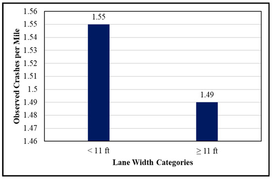
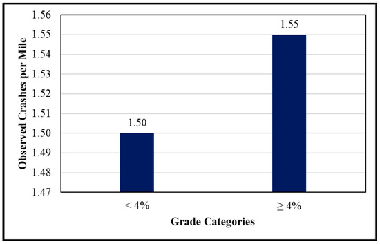
The CART results regarding lane width and grade were trivial as the analysis lumped all the data set into one class, thus providing no utility in classifying the variables. For these roadway characteristics, descriptive statistics, and engineering judgment were used to help in classifying the variables. For lane width, two classes were created: wider lanes with a lane width of 11 feet or wider, and narrower lanes with any lane width less than 11 feet. Figure 3 shows the observed crashes per mile for the two lane width classes used in the proposed models. For grade, the observed crashes per mile were plotted as a function of grade as shown in the bar chart in Figure 4. It is clear from this figure that the observed crashes notably increase when grade exceeds 4%. Therefore, two classes were used for classifying this variable: mild grade with a grade percentage less than 4%, and steep grade with a grade percentage equal or greater than 4%.

6.3. Proposed Models

Multivariate ordinary least squares linear regression analysis was used in developing the proposed models for low-volume road network screening. First, the data were split randomly into two parts. The first part consisting of 80 percent of the data (about 680 miles) was used to develop or train the model while the second part with the remaining 20 percent (about 170 miles) was used for testing the accuracy of the model.

The open-source statistical software R was used for analysis. Two models were developed: one with traffic exposure and another without traffic exposure information. The first model, which incorporates traffic volume as an explanatory variable, is shown in Equation (4).

$$\ln (Exp)=-0.88 LW-0.34 SW+0.016 DD+0.001 V+0.24 DC-0.31 SS-0.21 FO$$

(4)

where, Exp = EB expected number of crashes per year, LW = lane width, SW = shoulder width, DD = driveway density, V = exposure (AADT), DC = degree of curvature, SS = side slope and FO = fixed objects.

This model has a coefficient of determination (adjusted R-squared) of 0.915. This indicates that the model can explain more than 92 percent of the variability of the EB expected number of crashes, which is relatively high given the classified format used for most of the variables in this model. All variable coefficients were found significant at the 95% confidence level. All variable coefficients exhibited logical relationships with the explanatory variable, i.e., the expected number of crashes, given the fundamentals of safety science. Important information about the regression output for the first model is shown in

Table 2. Regression output for the first model.

Variables	Coefficients	p-Value	Significance at 95 Percent Confidence Level
Lane Width (LW)	−0.88	<2 × 10−6	✓
Shoulder Width (SW)	−0.34	<2 × 10−6	✓
Driveway Density (DD)	0.016	<2 × 10−6	✓
Volume (V)	0.001	<2 × 10−6	✓
Degree of Curvature (DC)	0.24	<2 × 10−6	✓
Side Slope (SS)	−0.31	<2 × 10−6	✓
Few Fixed Objects (FO)	−0.21	<2 × 10−6	✓
Adjusted R-squared = 0.915

.

To account for situations where traffic volume data are not available to local agencies, regression analysis was conducted using the same dataset while excluding the AADT from the analysis. The model is shown in Equation (5) below.

$$\ln \left(Exp\right)=-0.53 LW-0.46 SW+0.02 DD+0.27 DC-0.28 SS-0.25 FO$$

(5)

where, Exp = EB expected number of crashes per year, LW = Lane width, SW = Shoulder width, DD = Driveway density, DC = Degree of curvature, SS = Side slope and FO = Fixed objects.

This model is very similar to the previous model in format, i.e., the logarithmic format for the dependent variable and the linear format for all independent variables. The coefficient of determination for this model is not much different from that of the previous model (0.9057). This indicates that dropping the AADT from the second model did not much affect the predictive ability of the model as the R-squared value did not change but slightly. All the coefficients for independent variables were found significant at the 95% confidence level. Again, all coefficients exhibit a logical relationship between the response variable and explanatory variables. Important information about the regression output for the no-volume model is shown in

Table 3. Regression output for the no-volume model.

Variables	Coefficients	p-Value	Significance at 95 Percent Confidence Level
Lane Width (LW)	−0.53	<2 × 10−6	✓
Shoulder Width (SW)	−0.46	<2 × 10−6	✓
Driveway Density (DD)	0.02	<2 × 10−6	✓
Degree of Curvature (DC)	0.27	<2 × 10−6	✓
Flat Side Slope (SS)	−0.28	<2 × 10−6	✓
Few Fixed Objects (FO)	−0.25	<2 × 10−6	✓
Adjusted R-squared = 0.905

.

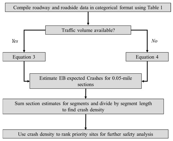
Figure 5 illustrates the major steps involved in the implementation of the proposed models in ranking priority sites as part of the network screening process.

6.4. Validation Results

The proposed models were validated using a different dataset to make sure that models perform reasonably well on other low-volume roads that are part of the network. The testing (validation) data contained 20 percent (about 170 miles) of the original dataset and was selected randomly. The expected crash numbers for the testing data were predicted using both the proposed models. To examine the predictive ability of the models, the mean bias error (MBE) and the root mean squared error (RMSE) were used. The MBE is the average of the differences between actual and predicted expected crashes. The MBE and RMSE are calculated as per Equations (6) and (7) below.

$$MBE=\frac{1}{n}\sum _1^n\left(\widehat{e}-e\right)$$

(6)

$$\mathrm{R}\mathrm{M}\mathrm{S}\mathrm{E}=\sqrt{\frac{\sum {(e-\widehat{e})}^2}{n}}$$

(7)

where, e = actual expected crashes, $\widehat{e}$ = predicted expected crashes, and n = number of data points.

For a more comprehensive validation, the mean, and the total of the actual and the predicted expected crashes were also calculated. All these parameters were also calculated for the training dataset and are provided in

Table 4. Validation metrics for the models.

	Training Data		Testing Data
	Mean	Total	Mean	Total
Actual Expected Crashes	0.087	1213	0.084	294
Model Estimate	0.085	1192	0.086	301
No Vol. Model Estimate	0.076	1057	0.077	268
MBE	−0.0015		0.0018
MBE (no volume)	−0.011		−0.007
RMSE	0.18		0.19
RMSE (no volume)	0.17		0.18

.

Considering the mean and the total expected crashes shown in Table 4, it is observed for the first model that the differences between the actual and predicted expected crashes are less than 5 percent for both the training and the testing datasets (2.3 and 1.7 percent for the training data; 2.4 and 2.4 percent for the testing data). These differences are considered particularly small given that all geometric variables are classified into a small number of categories. For the second model, the difference is about 12 percent (12.6 percent and 12.86 percent for the training; 8.3 percent and 8.8 percent for the testing datasets), which can be expected for a model that mostly uses categorical variables and lacks traffic exposure information. The small percentage differences between the mean and the total “actual” and “predicted” expected number of crashes suggest accurate prediction by the two models. The MBEs for both models are close to 0, suggesting that the model-predicted values are very close to the original values. The RMSEs are relatively small which supports the strong predictive ability of the models and is consistent with the high R-squared values discussed earlier.

7. Summary and Concluding Remarks

This paper presented a new method for network screening for local and low-volume roads. The method involves the use of regression models for predicting the expected number of crashes using roadway characteristics with or without the use of traffic exposure data. A key advantage of this method is that it does not require exact information or access to extensive databases as it employs classified roadway variables that can easily be compiled by staff of local agencies. Simple and basic tools like Google Maps can provide useful information for use as input to the proposed models. Another advantage of the proposed method is that it does not require extensive technical expertise for implementation. The prediction models consist of simple mathematical equations that can easily be understood and implemented. This would allow smaller local agencies (counties, townships, etc.) with limited technical expertise and lack of access to extensive databases to implement these models. One potential limitation in the proposed method is that the regression models developed may be state- or region-specific, and therefore the use of these models outside of Oregon would ideally require the use of local data in developing state-specific or region-specific models using the same approach followed in this research.

The two proposed models have R-squared values greater than 0.90 which suggests a very strong predictive ability and accurate predictions. The proposed models were also validated using a separate dataset and the results were deemed favorable overall. Further, the high R-squared values for the two models and the closeness of their numerical values (0.915 and 0.906) suggest that the contribution of crash history and traffic exposure in the estimation of the HSM EB expected number of crashes is not tangible on low-volume roads. This is consistent with the findings from a recent study [14] which found that the HSM EB method relies more on risk factors to estimate the EB expected number of crashes under low-volume conditions.

References

- National Highway Traffic Safety Administration (NHTSA). Rural Urban Comparison of Traffic Fatalities; NHTSA: Washington, DC, USA, 2018.
- Federal Highway Administration. (FHWA). Manual on Uniform Traffic Control Devices; FHWA: Washington, DC, USA, 2009. Available online: http://mutcd.fhwa.dot.gov/ (accessed on 28 March 2019).
- Gross, F.; Eccles, K.; Nabors, D. Low-Volume Roads and Road Safety Audits—Lessons Learned. Transp. Res. Rec. J. Transp. Res. Board 2011, 2213, 37–45. [Google Scholar] [CrossRef]
- Federal Highway Administration. (FHWA). Systemic Safety Project Selection Tool; FHWA: Washington, DC, USA, 2013. Available online: http://safety.fhwa.dot.gov/systemic/ (accessed on 25 March 2019).
- Minnesota Department of Transportation (MnDOT). Minnesota’s Systemic Approach Integrates Safety Performance into Investment Decisions for Local Roads. 2014. Available online: https://www.fhwa.dot.gov/innovation/everydaycounts/edc_4/pdf/case_study_mn_oct2014.pdf (accessed on 25 March 2018).
- North Dakota Department of Transportation. Local Road Safety Program, N.d. Available online: https://www.dot.nd.gov/sites/www/files/documents/VIEW_WesternRegion_Agency_TheodoreRooseveltNationalPark.pdf (accessed on 25 March 2018).
- Zhong, C.; Sisiopiku, V.P.; Ksaibati, K.; Zhong, T. Crash Prediction on Rural Roads. In Proceedings of the 3rd International Conference on Road Safety and Simulation, Purdue University, Indianapolis, IN, USA, 14–16 September 2011. [Google Scholar]
- Aguero-Valverdea, J.; Wub, K.K.; Donnell, E.T. A multivariate spatial crash frequency model for identifying sites with promise based on crash types. Accid. Anal. Prev. 2016, 87, 8–16. [Google Scholar]
- Al-Kaisy, A.; Veneziano, D.; Ewan, L.; Hossain, F. Risk Factors Associated with High Potential for Serious Crashes: Final Report; Report No. FHWA-OR-RD-16-05; Oregon Department of Transportation: Salem, OR, USA, 2015.
- Al-Kaisy, A.; Raza, S. A Novel Network Screening Methodology for Rural Low-Volume Roads. J. Transp. Technol. 2023, 13, 599–614. [Google Scholar] [CrossRef]
- Harris, D.; Durdin, P.; Brodieb, C.; Tate, F.; Gardener, R. A road safety risk prediction methodology for low volume rural roads. In Proceedings of the Australasian Road Safety Conference, Gold Coast, Australia, 14–16 October 2015. [Google Scholar]
- American Association of State Highway and Transportation Officials (AASHTO). Highway Safety Manual, 1st ed.; AASHTO: Washington, DC, USA, 2010. [Google Scholar]
- Cafiso, S.; Di Silvestro, G.; Persaud, B.; Ara Begum, M. Revisiting variability of dispersion parameter of safety performance for two-lane rural roads. Transp. Res. Rec. 2010, 2148, 38–46. [Google Scholar] [CrossRef]
- Al-Kaisy, A.; Huda, K.T. Empirical Bayes application on low-volume roads: Oregon case study. J. Saf. Res. 2022, 80, 226–234. [Google Scholar] [CrossRef] [PubMed]
- Elvik, R. The predictive validity of Empirical Bayes estimates of road safety. Accid. Anal. Prev. 2008, 40, 1964–1969. [Google Scholar] [CrossRef] [PubMed]
- Montella, A. A comparative analysis of hotspot identification methods. Accid. Anal. Prev. 2010, 42, 571–581. [Google Scholar] [CrossRef] [PubMed]
- Manepalli, U.R.R.; Bham, G.H. An evaluation of performance measures for hotspot identification. J. Transp. Saf. Secur. 2016, 8, 327–345. [Google Scholar] [CrossRef]
- Šenk, P.; Ambros, J.; Pokorný, P.; Striegler, R. Use of Accident Prediction Models in Identifying Hazardous Road Locations. Trans. Transp. Sci. 2012, 5, 223–232. [Google Scholar] [CrossRef]
- Abebe, M.T.; Belayneh, M.Z. Identifying and Ranking Dangerous Road Segments a Case of Hawassa-Shashemene-Bulbula Two-Lane Two-Way Rural Highway, Ethiopia. J. Transp. Technol. 2018, 8, 151–174. [Google Scholar] [CrossRef]
- Dixon, K.; Monsere, C.; Xie, F.; Gladhill, K. Calibrating the Future Highway Safety Manual Predictive Methods for Oregon State Highways; Final Report, SPR 684OTREC-RR-12-02; Oregon Department of Transportation: Salem, OR, USA, 2012.
- De’ath, G.; Fabricius, K.E. Classification and regression trees: A powerful yet simple technique for ecological data analysis. Ecology 2000, 81, 3178–3192. [Google Scholar] [CrossRef]
Disclaimer/Publisher’s Note: The statements, opinions and data contained in all publications are solely those of the individual author(s) and contributor(s) and not of MDPI and/or the editor(s). MDPI and/or the editor(s) disclaim responsibility for any injury to people or property resulting from any ideas, methods, instructions or products referred to in the content. |
© 2024 by the authors. Licensee MDPI, Basel, Switzerland. This article is an open access article distributed under the terms and conditions of the Creative Commons Attribution (CC BY) license (https://creativecommons.org/licenses/by/4.0/).