Article

A Hybrid LSTM-CPS Approach for Long-Term Prediction of Train Delays in Multivariate Time Series

1
School of Computing and Information Technology, University of Wollongong, Wollongong, NSW 2522, Australia
2
SMART Infrastructure Facility, University of Wollongong, Wollongong, NSW 2522, Australia
3
School of Civil, Mining and Environmental, University of Wollongong, Wollongong, NSW 2522, Australia
4
School of Information and Engineering, Lanzhou University, Lanzhou 730000, China
5
School of Electrical and Information Engineering, The University of Sydney, Sydney, NSW 2006, Australia
6
CSIRO’s Data61, Sydney, NSW 2015, Australia
7
School of Computer Science, Beijing Institute of Technology, Beijing 100811, China
8
School of Computer Science and Engineering, Xi’an University of Technology, Xi’an 710048, China
*
Author to whom correspondence should be addressed.
Future Transp. 2021, 1(3), 765-776; https://doi.org/10.3390/futuretransp1030042
Submission received: 22 October 2021 / Revised: 27 November 2021 / Accepted: 1 December 2021 / Published: 3 December 2021

Abstract

:
In many big cities, train delays are among the most complained-about events by the public. Although various models have been proposed for train delay prediction, prior studies on both primary and secondary train delay prediction are limited in number. Recent advances in deep learning approaches and increasing availability of various data sources has created new opportunities for more efficient and accurate train delay prediction. In this study, we propose a hybrid deep learning solution by integrating long short-term memory (LSTM) and Critical Point Search (CPS). LSTM deals with long-term prediction tasks of trains’ running time and dwell time, while CPS uses predicted values with a nominal timetable to identify primary and secondary delays based on the delay causes, run-time delay, and dwell time delay. To validate the model and analyse its performance, we compare the standard LSTM with the proposed hybrid model. The results demonstrate that new variants outperform the standard LSTM, based on predicting time steps of dwell time feature. The experiment results also showed many irregularities of historical trends, which draws attention for further research.

1. Introduction

Recent trends have showed a great need for the adoption of intelligent transport systems (ITS), especially in metropolises. This would generate various impacts on both passenger transport and freight logistics [1,2,3], which helps to reduce traffic emissions and energy consumption [4,5,6,7]. Moreover, train transport plays an essential role in a multimodal transport system for both inter-city and intra-city travelers. The train timetabling problem (TTP) aims to find a periodic timetable that provides a preoperational schedule for a set of trains and follows operational constraints [8,9]. Nevertheless, train delays may cause a scheduled timetable to become infeasible and lead to inefficient operations, poor services, and longer travel time to complete passenger journeys. Therefore, accurate prediction of train delays is a vital task for control of railway traffic. Traditional model-driven methods have been widely studied in train delay prediction, such as micro and macro simulation methods [10,11,12]. In simulation-based approaches, each simulation model requires numerous parameters. Due to time-varying operating conditions and interactions between different subsystems subject to infrastructure and operational rules, parameter calibration is a significant challenge in building a successful simulation model [13].
In railway transport systems, diverse data are collected from various sources containing sensors, smart cards, Global Positioning System (GPS), and video detectors. With the fast development of big data techniques, many studies have focused on machine learning algorithms to learn the general rules that map a set of inputs to outputs in spatio-temporal prediction. State-of-the-art delay prediction models can be divided into two categories: deterministic and stochastic prediction models. Deterministic prediction models, such as neural networks and ensemble learning, usually use past observations to produce a fixed best-estimate value, while stochastic prediction models such as Bayesian networks consider a probability distribution. A diversity of factors may cause train delays. For example, primary congestion predictive factors have the most significant impacts on congestion delay, including meets, passes, and overtakes [14]. Hence, although the train delay can be reduced, it cannot be avoided. The types of train delay prediction can be classified as real-time/short-term, and medium-/long-term prediction [15]. Train delays can be classified as primary and secondary delays [16]. Due to the effects of the delay propagation, a primary delay (an initial delay) occurring at a station often causes secondary delays (or knock-on delays) at subsequent stations.
Ref. [17] proposed a fuzzy Petri net (FPN) model to simulate train primary delays and knock-on delays in a railway system. Ref. [18] developed an artificial neural network (ANN) to predict delays of passenger trains. The application of support vector regression (SVR) achieved better performance than ANN [19]. Ref. [20] used a microscopic graph model for online prediction of event times based on a directed acyclic graph (DAG) with dynamic arc weights. Ref. [21] presented and compared the accuracy and computation time of global and local data-driven approaches for calibrating the microscopic prediction model in real-time. Ref. [22] constructed a decision tree to estimate the root causes and effects of knock-on delays. Ref. [23] established a dynamic train delay prediction system (DTDPS) based on shallow extreme learning machine (SELM) and deep extreme learning machine (DELM), which used a repeated learning process with historical train movement data and exogenous weather data for long-term prediction of train delays in a large-scale railway network.
Furthermore, Ref. [24] demonstrated a dynamic stochastic model that predicts conditional probability distributions of train delays in real-time. The model applied prior probabilities for parent nodes to update calibration results of Bayesian networks with the probability distribution and regression coefficients for every two related events. Similarly, Ref. [25] presented an algorithmic performance comparison of three Bayesian network training methods, including hill climbing, primitive linear, and hybrid structures. The hybrid structure combined data-driven approaches with some domain knowledge which outperformed the other models. Ref. [26] proposed a data-driven ensemble forecasting model for medium-term prediction of train delays. The model combined a context-aware Random Forest (RF) and a regression with a mesoscopic simulation-based approach. Ref. [27] indicated a bi-level RF approach to estimate near-term train delays. The approach incorporated an RF classifier for predicting the increase, decrease, or lack of change for a current delay at the primary level, and three RF regression models for measuring the change in delay at the secondary level. Ref. [28] proposed a generic delay prediction framework to establish a connection between expert knowledge with long short-term memory (LSTM). The Convolutional Neural Network (CNN) [29], Gated Recurrent Unit (GRU) [30], and LSTM can be combined to form a more complex structure. In some circumstances, hybrid methods (e.g., Bidirectional LSTM and GRU-LSTM) can reach a better performance than a simple structure for unlocking hidden patterns in data [31,32]. Ref. [33] showed a hybrid method to merge the knowledge of the network and the experience of the operators, and data-driven models based on operational data and exogenous information to predict running time, dwell time, train delay, penalty cost, and train overtaking. Ref. [34] presented a train spatio-temporal graph convolutional network (TSTGCN), which included weather variables as input variables to predict the number of delayed trains in a certain period. Ref. [15] proposed a rule-driven automation approach for multi-scenario real-time prediction, which consisted of a delay status labeling algorithm, resilience of section and resilience of station factors.
Although various models have been proposed for real-time or long-term train delay prediction, to the best of our knowledge, no prior work has applied a deep learning approaches to both primary and secondary delay prediction. In this paper, we propose a comprehensive architecture of deep learning methodology for long-term train delay prediction. The contributions of this paper are summarized as: (1) The causes of train delay, run-time delay and dwell delay are accurately investigated and distinguished. We aim to predict the running time and dwell time instead of performing train delay prediction directly. (2) Several machine learning models are trained and evaluated using General Transit Feed Specification (GTFS) time series dataset, and the experimental results show the effectiveness and efficiency of the proposed model. (3) Detailed guidelines on generating multivariate regression features and building a robust train delay forecasting system are introduced.
The remainder of the paper is organized as follows. Section 2 describes the train delay and interprets the causes of train delays; this section also introduces a preliminary critical point search (CPS) classification algorithm, supervised learning setting, and multivariate time series models. Section 3 of experiments discusses static and real-time train operation data fusion, evaluation methods, and prediction results. Section 4 presents a summary of this study.

2. Methodology

2.1. Train Delay Problem

A railway network can be expressed as a graph. The nodes on the graph present a series of stations. Passenger trains are typically run along railway tracks based on regular schedules. Each trip has an original station, a destination station, and some intermediate stations. In this paper, we consider a train T serving a series of stations S m , where S m   { S 1 , S 2 , , S l } . The train operational variables and spatio-temporal variables are defined as actual arrival time a t a   ( T , S m ) , actual departure time a t d   ( T , S m ) , scheduled arrival time s t a   ( T , S m ) , scheduled departure time s t d   ( T , S m ) , actual dwell time d a   =   a t d   ( T , S m )     a t a ( T , S m ) , and actual running time r a   =   a t a   ( T , S m )     a t d   ( T , S m     1 ) , respectively. If the difference of arrival time a t a   ( T , S m )     s t a   ( T , S m ) and departure time a t d   ( T , S m )     s t d   ( T , S m ) are more than 30 s and 60 s, an arrival delay and a departure delay occur at the corresponding station, respectively. Furthermore, each trip has a real-time record from which it is to retrieve the category of the trip. Each station has a unique sequence value from which it is to specify the order of the stations.

2.2. Critical Point Search Classification

Classifying the predicted data by train delay categories helps us to understand the model output. A classification algorithm is required to incorporate domain knowledge to extract the information from the output of a predictive model. CPS is a rule-based classification method to search primary, secondary and on-time points [28]. It can be extended to identify those train stations that cause major disruption to services. If it is able to predict the primary delay and secondary delay, we can reduce or avoid delays in advance. The CPS algorithm (Algorithm 1) has If–Then rules to identify the primary delay and secondary delay at the corresponding arrival stations from arrival delays of a trip list A D S m . By comparing the difference of arrival delays of adjacent train stations, the two types of delay points or on-time running points can be added to the lists,   L 1 ,   L 2   and   L 3 , where L 1 denotes a list of on-time running points, L 2 represents a list of secondary delay points, and L 3 is a list of primary delay points. The algorithm also can be applied to departure delay calculation.
Algorithm 1. CPS Algorithm
Input: Given a trip R with a set of arrival delay A D S m   =   ( A D S 1 , A D S 2 A D S l ) ,
and pre-defined thresholds   V 1 ,   V 2
Output: L 1 , L 2 , L 3
m = 0
For each arrival delay   ( A D S 1 , A D S 2 A D S l )
     if  A D S m + 1 < V 1 :
        L 1 . a d d ( A D S m + 1 )
     else:
       if  A D S m + 1     A D S m     V 2 :
          L 3 . a d d ( A D S m + 1 )
       else:
          L 2 . a d d ( A D S m + 1 )
End for

2.3. Supervised Learning Setting

Figure 1 demonstrates the architecture of data visualization for the feature generation process. For a sequence-to-sequence model [35], the time series data as inputs are shown by X d , where d   presents the number of samples (or stations) for each sequential matrix. The illustration of X d is shown in Figure 1 as a set of sequential matrices. The train delays,   X d , which can be indicated in vector form as X d   =   [ X t d , X t + 1 d , X t + 2 d , X t   +   n     1 d ] . X d with a time-step is from t to   t + n     1 . For example, in X t d , the time steps of the lag   w are from t     w   +   1 to t , which can be expressed explicitly in matrix form as
X t d   =   [ x t 1 x t 2 x t d x t     1 1 x t     1 2 x t     1 d x t     w   +   1 1 x t     w   +   1 2 x t     w   +   1 d ]

2.4. Multivariate Time Series Forecasting Model

This section demonstrates the design and development of a comprehensive LSTM-CPS network architecture for multivariate delay predictions. As demonstrated in Figure 2, a multivariate forecasting model is composed of Long Short-Term Memory (LSTM), two rectified linear units (ReLU), two dense layers, a dropout layer, and a CPS component. The last dense layer outputs a range of future values. Additionally, the outputs are passed to the CPS as inputs in a list. In addition, the CPS classifies the predicted values, which include not only the primary delays, secondary delays, and on-time running of corresponding stations, but also the status of the entire trip in the future at a given history. Furthermore, different machine learning methods and model hyperparameters are introduced in the following content.
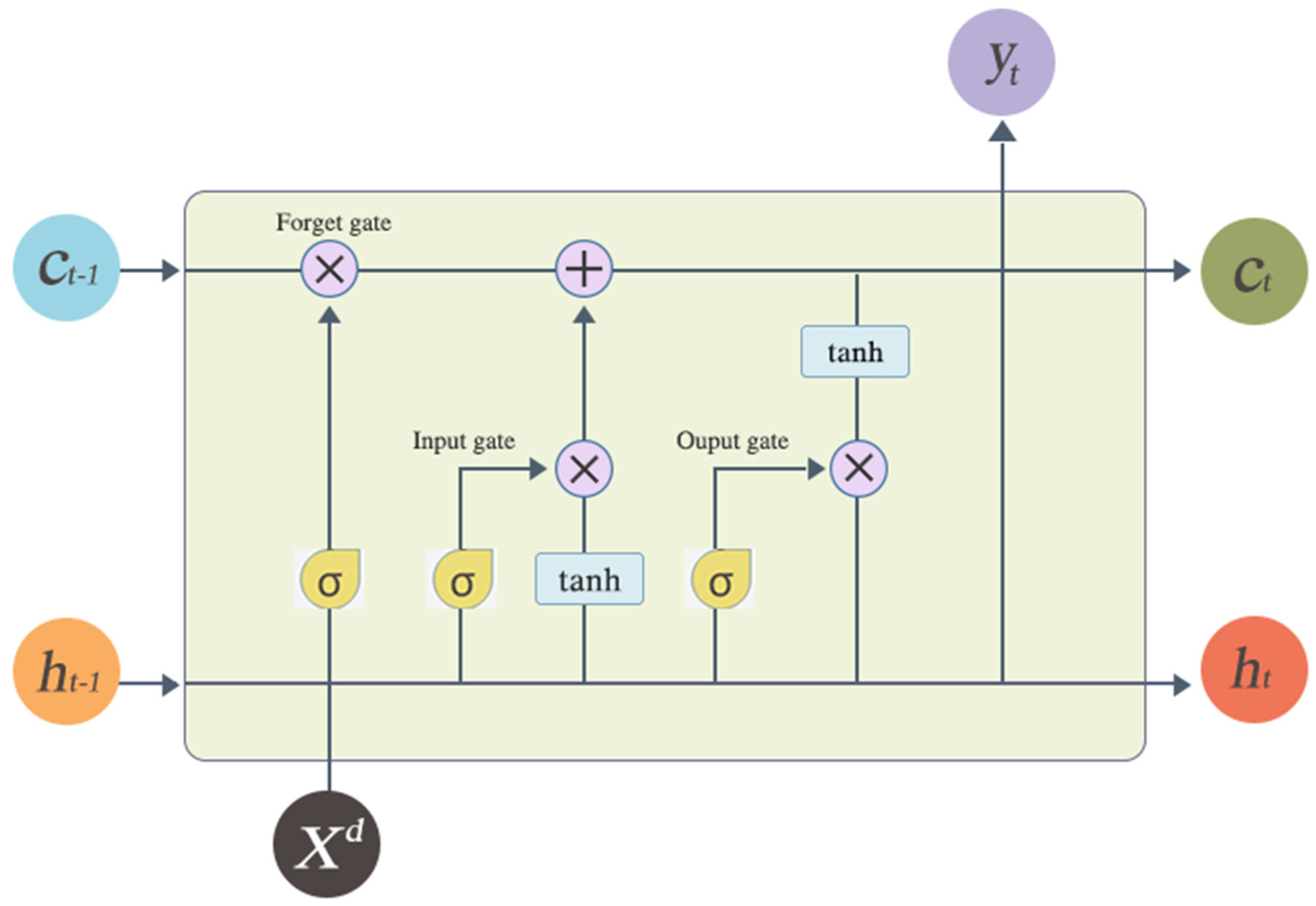
Ref. [36] introduced an LSTM network, which consisted of an input gate i , a forget gate f , a cell c , and an output gate o . As shown in Figure 3, a standard LSTM contains two types of states: the long-term state and the short-term state. Specifically, the short-term state h t     1 and the current input X d are fed to three Sigmoid functions and a t a n h activation function. Moreover, the long-term state c t     1 traverses the network to c t . Firstly, it drops some memories in the forget gate, secondly, some new memories are added to the input gate by using the addition operation. Additionally, then the long-term state is passed through the t a n h activation function. Finally, the output gate filters the results, generating the output y t and the short-term state h t ( y t is equal to h t at the time step). W x i , W x f , W x c , and W x o denote the weight matrices that connect the input to the corresponding gates. W h i , W h f ,   W h c , and W h o present the weight matrices that connect the hidden vector to the corresponding gates.   b i ,   b f , b c , and b o refer to bias vectors. In this paper, we follow the version of fully connected LSTM (FC-LSTM) from [37]. The key equations of LSTM are indicated in Equation (2) below, where σ is the logistic sigmoid function and the operator ‘ ’ is the Hadamard product:
i t   =   σ ( W x i   X d + W h i h t     1 + W c i c t     1   +   b i )
f t   =   σ ( W x f   X d + W h f h t     1   +   W c f c t     1   +   b f )
c t   =   f t c t     1   +   i t t a n h ( W x c X d + W h c h t     1 + b c )
o t   =   σ ( W x o   X d + W h o h t     1   +   W c o c t + b o )
h t   =   o t t a n h ( c t )
Multiple LSTMs can be combined to build a more complex network structure. Such a model is capable of solving real-world sequence learning problems. In some cases, it generates good outcomes where the model presents performance improvement, rather than a simple structure for discovering trends, seasonality, and cyclicity patterns [31,32]. Since the absolute error is more robust to outliers, we use an L1 loss to measure the performance of our model. Hence, the loss function of the hybrid LSTM-CPS learning architecture for multivariate prediction tasks can be expressed as
h ^ n   =   arg m i n 1 n i   =   1 n l | y i     h ( X d ) i |
where h ^ n are training loss and validation loss; y i is the ground truth; and h ( X d ) i expresses the prediction of the model.
We sum up the main characteristics of our hybrid LSTM-CPS learning architecture in the following.
  • The CPS algorithm can obtain primary delay and secondary delays on each trip, which presents essential time–space relationships in the status of the railway network.
  • A multivariate LSTM model is developed to estimate regression coefficients for multiple stations.
  • The hybrid LSTM-CPS is a batch-based prediction architecture to process structured time series. It is not only able to have multi-inputs and multi-outputs (MIMO) features but is also able to be extended to tackle spatio-temporal sequence learning tasks. Notably, this architecture allows deep learning models to reach higher efficiency and accuracy for large-scale railway networks.

3. Experiments

3.1. Data Description

To evaluate the performance of the proposed LSTM-CPS network architecture, comprehensive experiments have been conducted on the fused train dataset from the Transport for NSW’s open data hub. The dataset contains 161-day historical observations of the trip ‘600D’ (8:30 a.m.–9:00 a.m.) in the period 11 April to 21 November in 2019. The line is from Sydney’s Bondi Junction Station, Platform 1 to Hurstville Station, Platform 4 in the Monday to Friday morning peak hours. Meanwhile, the corresponding schedule data and geographical information are obtained in the same time period. This dataset includes scheduled arrival time, scheduled departure time, station name, longitude, and latitude.
GTFS offers detailed schedules and associated geographic information in an open-source data format [38]. A data extraction and pre-processing tool is implemented to obtain real-time information from a GTFS-realtime application programming interface (API) provided by Transport for NSW. This dataset contains arrival delay, departure delay, and stop ID.
The proposed learning architecture is implemented in Python using the TensorFlow Framework [39] and trained using the Adam algorithm [40].

3.2. Evaluation Metrics

In this study, the proposed model is evaluated based on five standard metrics: mean absolute error (MAE), root mean square error (RMSE), mean absolute percentage error (MAPE), coefficient of determination ( R 2 ) and Adjusted R-squared ( Adjusted   R 2 ) values, as shown in Equations (4)–(8), where y t is the actual value at time step t , y ^ t is the predicted value, y ¯ is the mean of the observed values of the dependent variable, n is the total sample size, and k is the number of predictors.
MAE   =   1 n i   =   1 n | y t     y ^ t |
RMSE   =   1 n i   =   1 n ( y t     y ^ t ) 2
MAPE   =   1 n i   =   1 n ( y t     y ^ t y t   )
R 2   =   1     i   =   1 n ( y t     y ^ t ) 2 i   =   1 n ( y t     y ¯ ) 2
Adjusted   R 2   =   1     n     1 n     ( k   +   1 ) ( 1     R 2 )
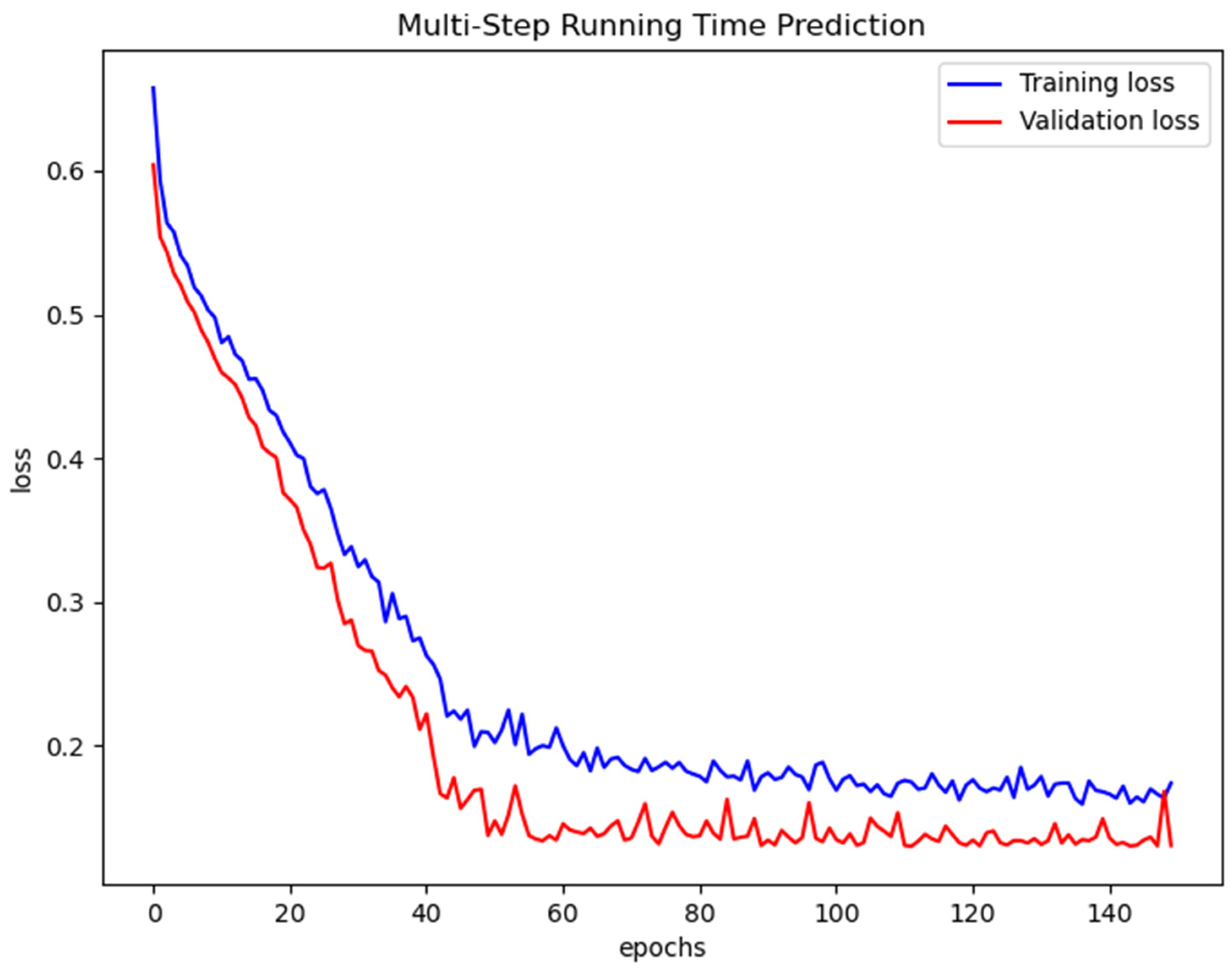
For training a deep learning model, the first 100 days of the 161-day dataset is compiled as the training dataset and the remaining data is used as the validation dataset, roughly 70/30 split. According to the network structure of Figure 2, we select a batch size of 32 and 150 epochs as the parameters of the training model. Figure 4 illustrates the loss during the training and validation procedures. Both the training loss and validation loss converge after approximately 60 epochs. In this experiment, the batch size and the number of epochs are set as 32, and 60 for running time prediction and 20 for dwell time prediction, respectively. MAE is exploited as a loss function in the training process. Since the performance difference between training and validation is acceptable, the model does not overfit the training data.

3.3. Model Comparison

Figure 5 reports the performance of our proposed models with different LSTM variants or combinations of CNN, LSTM, and GRU for predicting one day ahead running time of seven intermediate stations from the trip ‘600D’. All x-axes express the corresponding metrics. The y-axis of RMSE and MAE shows the error in seconds; the y-axis of MAPE denotes the proportion of the error; the y-axis on the right of the figure represents the training time (seconds) of the corresponding models. In addition to Random Forest, other models do not show significant differences in model performance. The standard LSTM reaches the lowest MAPE value. Random Forest reaches minimum training time. In summary, the standard LSTM has a sufficiently good prediction performance in terms of all validation metrics.
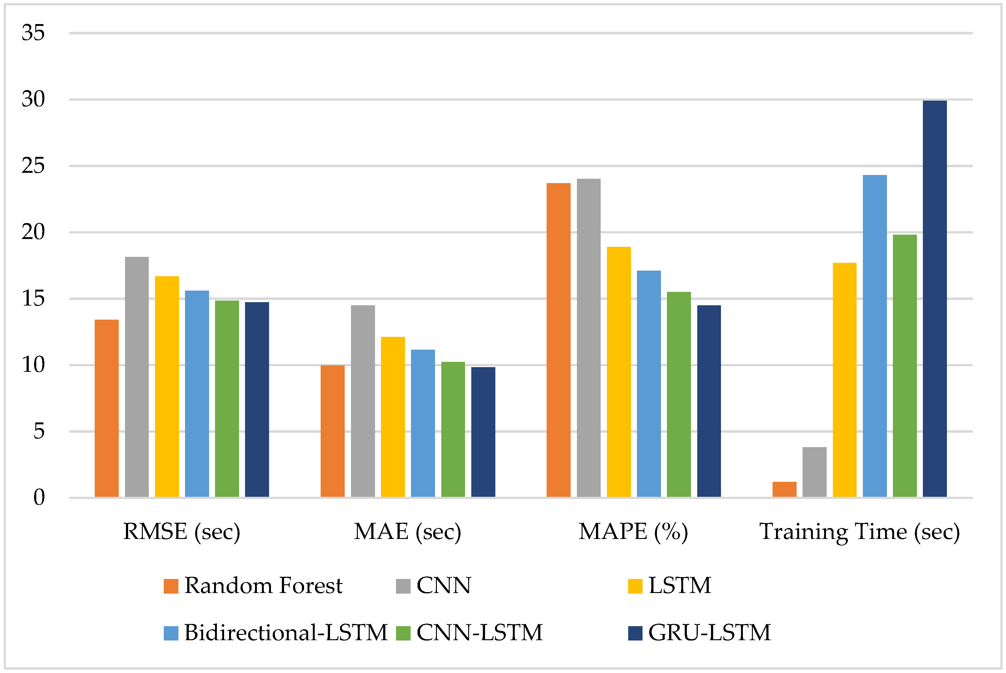
The expressions for the x-axis and y-axis in Figure 6 are the same as in Figure 5, but the performance of the proposed models for dwell time prediction, and estimation accuracies in terms of all validation metrics with one day ahead are reported instead. Random Forest provides the highest accuracy in RMSE. For MAE, and MAPE, GRU-LSTM achieves the highest prediction accuracy; however, the time cost of the model is the highest. To sum up, compared with the LSTM variants, the Random Forest, standard LSTM, and CNN have more substantial errors and less training time. LSTM variants do not have significant performance differences.
Table 1 and Table 2 demonstrate the results of the proposed models. In Table 1, it is observed that Random Forest has the lowest training time. For 7-steps ahead prediction, LSTM achieves lower MAE and MAPE, compared to others. However, in Table 2, GRU-LSTM performs well for 7-steps ahead prediction. Additionally, the differences between all LSTM variants in performance are slight.
As shown in Figure 1, the trend volatility line of running time (red line) is more regular than the dwell time (green line). It shows that dwell time demonstrates higher randomness, due to delays caused by the non-fixed daily number of passengers or uncertain events that occurred at the corresponding train station. For run-time prediction, a simpler neural network model can quickly achieve good performance. For dwell time prediction, a more complex network structure can better capture hidden patterns and trends in the dataset.
To establish a real-world deep learning application, we also need to balance or even trade-off accuracy and training time and prevent overfitting of the model. Time series data have a certain degree of randomness. In some cases, certain model approaches a high accuracy, but overfitting occurs. It dramatically reduces the portability of the model. In addition to accurately assessing the maximum predictability of the dataset, in further studies, we need to explore automated model selection techniques to identify an appropriate predictor for the corresponding inputs.
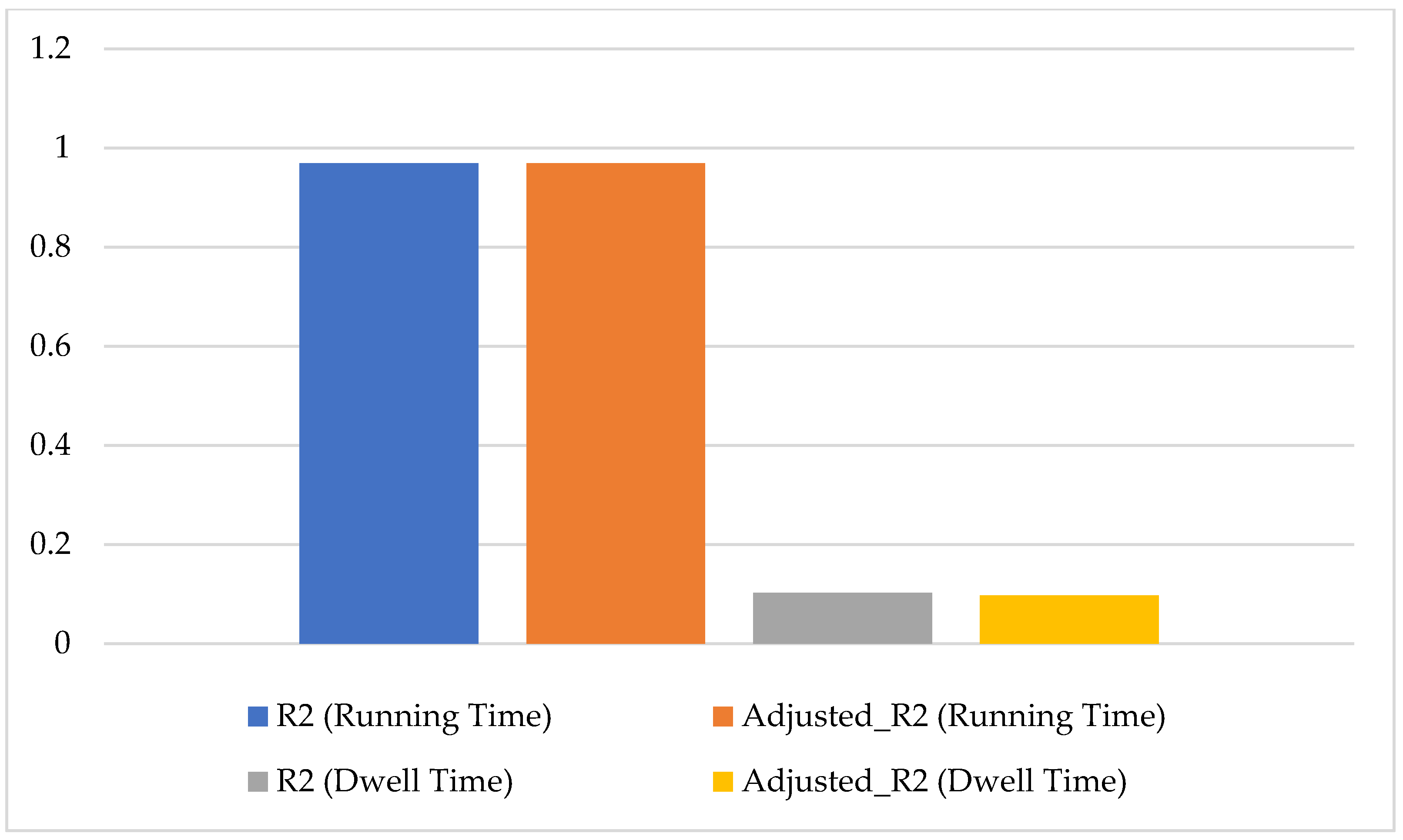
Finally, we compared R-squared and Adjusted R-squared values resulting from the proposed models. Figure 7 reports a standard LSTM for running time prediction and best performance LSTM variants for dwell time prediction from one day ahead. Moreover, a baseline model predicts y ¯ , which has default values R 2   =   0 and R adj 2   =   0 . The paper compares the proposed standard LSTM and LSTM variants against the baseline model. The result shows that the running time has a small variation with high accuracy, which is to a great extent explained by predictors in the standard LSTM. The proposed architecture presents reliable predictive power. Additionally, the running time shows a weak dependence on train delays. Data visualization in Figure 1 indicates that most trains run at their best performance regardless of departure delays. The impact of running time on the peak hours of workdays is also weak. Therefore, dwell time is more closely related to arrival delays.
Figure 7 shows the R-squared and Adjusted R-squared values for one day ahead. There is an amount of unexplainable uncertainty, which is represented by R-squared and Adjusted R-squared. It can be observed that most of the randomness comes from the dwell time. Our model chooses the appropriate numbers of epochs to achieve the smallest value h ^ n through the method of Figure 4. If we increase the number of epochs to reach the higher values of R-squared and Adjusted R-squared, it will cause the model to be overfitting or underfitting.

4. Conclusions

This paper dealt with establishing a hybrid deep learning architecture for long-term train delay prediction using real-world data collected from different sources in an Internet of Things (IoT)-empowered public transport agency. The LSTM and LSTM variants could achieve high prediction accuracy by exploiting the long-term temporal dependency patterns. Several machine learning models, including Random Forest, CNN, LSTM, and LSTM variants, were applied to predict the running time and dwell time. Moreover, CPS utilizes experimental results to implement the predicted primary delays and the predicted secondary delays. The solution can be directly used for long-term prediction in urban railway systems. In future work, a stochastic probability model, such as a conditional Bayesian model, can be used to adjust the delay information of the entire network in real-time. Meanwhile, we will provide more comparisons with stronger baselines such as kernel methods, as meaningful future work.

Author Contributions

J.W., J.S. and B.D. conceived and designed the experimental setup and algorithms; J.W. developed main approaches; performed the experiments; Q.W. contributed data pre-processing and benchmarking data; and C.C. provided raw data. W.W. and Q.Z. contributed to review and editing. All authors contributed to the discussion and analysis of the research and to the writing of the paper. All authors have read and agreed to the published version of the manuscript.

Funding

The authors gratefully acknowledge the support of the Natural Science Foundation of Shaanxi Province of China(2021JM-344) and National Key R&D Program of China under Grant, No. 2020YFC0832500. Wu also gratefully acknowledges financial support from the China Scholarship Council (201608320168).

Institutional Review Board Statement

Not Applicable.

Informed Consent Statement

Not Applicable.

Data Availability Statement

Not Applicable.

Conflicts of Interest

The authors declare no conflict of interest. The funders had no role in the design of the study; in the collection, analyses, or interpretation of data; in the writing of the manuscript, or in the decision to publish the results.

References

  1. Konstantakopoulos, G.D.; Gayialis, S.P.; Kechagias, E.P.; Papadopoulos, G.A.; Tatsiopoulos, I.P. A Multiobjective Large Neighborhood Search Metaheuristic for the Vehicle Routing Problem with Time Windows. Algorithms 2020, 13, 243. [Google Scholar] [CrossRef]
  2. Kechagias, E.P.; Gayialis, S.P.; Konstantakopoulos, G.D.; Papadopoulos, G.A. Traffic flow forecasting for city logistics: A literature review and evaluation. Int. J. Decis. Support Syst. 2019, 4, 159–176. [Google Scholar] [CrossRef]
  3. Bernardo, M.; Du, B.; Pannek, J. A simulation-based solution approach for the robust capacitated vehicle routing problem with uncertain demands. Transp. Lett. 2021, 13, 664–673. [Google Scholar] [CrossRef]
  4. Kechagias, E.P.; Gayialis, S.P.; Konstantakopoulos, G.D.; Papadopoulos, G.A. An Application of an Urban Freight Transportation System for Reduced Environmental Emissions. Systems 2020, 8, 49. [Google Scholar] [CrossRef]
  5. Vieira, B.O.; Guarnieri, P.; Nofal, R.; Nofal, B. Multi-Criteria Methods Applied in the Studies of Barriers Identified in the Implementation of Reverse Logistics of E-Waste: A Research Agenda. Logistics 2020, 4, 11. [Google Scholar] [CrossRef]
  6. Mohtashami, Z.; Aghsami, A.; Jolai, F. A green closed loop supply chain design using queuing system for reducing environmental impact and energy consumption. J. Clean. Prod. 2020, 242, 118452. [Google Scholar] [CrossRef]
  7. Sheng, M.S.; Sreenivasan, A.V.; Sharp, B.; Du, B. Well-to-wheel analysis of greenhouse gas emissions and energy consumption for electric vehicles: A comparative study in Oceania. Energy Policy 2021, 158, 112552. [Google Scholar] [CrossRef]
  8. Caprara, A.; Fischetti, M.; Toth, P. Modeling and solving the train timetabling problem. Oper. Res. 2002, 50, 851–861. [Google Scholar] [CrossRef]
  9. Kang, L.; Wu, J.; Sun, H.; Zhu, X.; Wang, B. A practical model for last train rescheduling with train delay in urban railway transit networks. Omega 2015, 50, 29–42. [Google Scholar] [CrossRef]
  10. Frede, L.; Müller-Hannemann, M.; Schnee, M. Efficient on-Trip Timetable Information in the Presence of Delays. In Proceedings of the 8th Workshop on Algorithmic Approaches for Transportation Modeling, Optimization, and Systems (ATMOS’08), 2008. Available online: https://drops.dagstuhl.de/opus/volltexte/2008/1584/pdf/08002.Frede.1584.pdf (accessed on 12 November 2021).
  11. Berger, A.; Gebhardt, A.; Müller-Hannemann, M.; Ostrowski, M. Stochastic Delay Prediction in Large Train Networks. In Proceedings of the 11th Workshop on Algorithmic Approaches for Transportation Modelling, Optimization, and Systems, 2011. Available online: https://drops.dagstuhl.de/opus/volltexte/2011/3270/pdf/10.pdf (accessed on 12 November 2021).
  12. Zhang, Y.; Li, R.; Guo, T.; Li, Z.; Wang, Y.; Chen, F. A conditional Bayesian delay propagation model for large-scale railway traffic networks. In Proceedings of the Australasian Transport Research Forum, ATRF 2019-Proceedings, Canberra, Australia, 30 September–2 October 2019. [Google Scholar]
  13. Shi, R.; Xu, X.; Li, J.; Li, Y. Prediction and analysis of train arrival delay based on XGBoost and Bayesian optimization. Appl. Soft Comput. 2021, 109, 107538. [Google Scholar] [CrossRef]
  14. Gorman, M.F. Statistical estimation of railroad congestion delay. Transp. Res. Part E Logist. Transp. Rev. 2009, 45, 446–456. [Google Scholar] [CrossRef]
  15. Wu, J.; Wang, Y.; Du, B.; Wu, Q.; Zhai, Y.; Shen, J.; Zhou, L.; Cai, C.; Wei, W.; Zhou, Q. The Bounds of Improvements toward Real-Time Forecast of Multi-Scenario Train Delays. IEEE Trans. Intell. Transp. Syst. 2021, 1–12. [Google Scholar] [CrossRef]
  16. Yamamura, A.; Koresawa, M.; Adachi, S.; Tomii, N. Identification of Causes of Delays in Urban Railways. Comput. Railw. 2013, 13, 403–414. [Google Scholar]
  17. Milinković, S.; Marković, M.; Vesković, S.; Ivić, M.; Pavlović, N. A fuzzy Petri net model to estimate train delays. Simul. Model. Pract. Theory 2013, 33, 144–157. [Google Scholar] [CrossRef]
  18. Yaghini, M.; Khoshraftar, M.M.; Seyedabadi, M. Railway Passenger Train Delay Prediction via Neural Network Model. J. Adv. Transp. 2013, 47, 355–368. [Google Scholar] [CrossRef]
  19. Marković, N.; Milinković, S.; Tikhonov, K.S.; Schonfeld, P. Analyzing passenger train arrival delays with support vector regression. Transp. Res. Part C Emerg. Technol. 2015, 56, 251–262. [Google Scholar] [CrossRef]
  20. Kecman, P.; Goverde, R.M. Online data-driven adaptive prediction of train event times. IEEE Trans. Intell. Transp. Syst. 2014, 16, 465–474. [Google Scholar] [CrossRef]
  21. Kecman, P.; Goverde, R.M. Predictive Modelling of Running and Dwell Times in Railway Traffic. Public Transp. 2015, 7, 295–319. [Google Scholar] [CrossRef] [Green Version]
  22. Lee, W.-H.; Yen, L.-H.; Chou, C.-M. A delay root cause discovery and timetable adjustment model for enhancing the punctuality of railway services. Transp. Res. Part C Emerg. Technol. 2016, 73, 49–64. [Google Scholar] [CrossRef]
  23. Oneto, L.; Fumeo, E.; Clerico, G.; Canepa, R.; Papa, F.; Dambra, C.; Mazzino, N.; Anguita, D. Dynamic Delay Predictions for Large-Scale Railway Networks: Deep and Shallow Extreme Learning Machines Tuned via Thresholdout. IEEE Trans. Syst. Man Cybern. Syst. 2017, 47, 2754–2767. [Google Scholar] [CrossRef]
  24. Corman, F.; Kecman, P. Stochastic Prediction of Train Delays in Real-Time using Bayesian Networks. Transp. Res. Part C Emerg. Technol. 2018, 95, 599–615. [Google Scholar] [CrossRef] [Green Version]
  25. Lessan, J.; Fu, L.; Wen, C. A hybrid Bayesian network model for predicting delays in train operations. Comput. Ind. Eng. 2019, 127, 1214–1222. [Google Scholar] [CrossRef]
  26. Nair, R.; Hoang, T.L.; Laumanns, M.; Chen, B.; Cogill, R.; Szabó, J.; Walter, T. An Ensemble Prediction Model for Train Delays. Transp. Res. Part C Emerg. Technol. 2019, 104, 196–209. [Google Scholar] [CrossRef]
  27. Nabian, M.A.; Alemazkoor, N.; Meidani, H. Predicting Near-Term Train Schedule Performance and Delay using Bi-Level Random Forests. Transp. Res. Rec. 2019, 2673, 564–573. [Google Scholar] [CrossRef]
  28. Wu, J.; Zhou, L.; Cai, C.; Dong, F.; Shen, J.; Sun, G. Towards a General Prediction System for the Primary Delay in Urban Railways. In Proceedings of the 2019 IEEE Intelligent Transportation Systems Conference (ITSC), Auckland, New Zealand, 27–30 October 2019; pp. 3482–3487. [Google Scholar]
  29. LeCun, Y.; Bengio, Y. Convolutional Networks for Images, Speech, and Time Series. Handb. Brain Theory Neural Netw. 1995, 3361, 255–258. [Google Scholar]
  30. Cho, K.; van Merriënboer, B.; Gulcehre, C.; Bahdanau, D.; Bougares, F.; Schwenk, H.; Bengio, Y. Learning Phrase Representations using RNN Encoder–Decoder for Statistical Machine Translation. In Proceedings of the 2014 Conference on Empirical Methods in Natural Language Processing (EMNLP), Doha, Qatar, 25–29 October 2014. [Google Scholar]
  31. Lin, T.; Guo, T.; Aberer, K. Hybrid Neural Networks for Learning the Trend in Time Series. In Proceedings of the Twenty-Sixth International Joint Conference on Artificial Intelligence, Melbourne, Australia, 19–25 August 2017; pp. 2273–2279. [Google Scholar] [CrossRef] [Green Version]
  32. Du, S.; Li, T.; Yang, Y.; Horng, S. Deep Air Quality Forecasting Using Hybrid Deep Learning Framework. IEEE Trans. Knowl. Data Eng. 2019, 33, 2412–2424. [Google Scholar] [CrossRef] [Green Version]
  33. Oneto, L.; Buselli, I.; Lulli, A.; Canepa, R.; Petralli, S.; Anguita, D. A dynamic, interpretable, and robust hybrid data analytics system for train movements in large-scale railway networks. Int. J. Data Sci. Anal. 2020, 9, 95–111. [Google Scholar] [CrossRef]
  34. Zhang, D.; Peng, Y.; Zhang, Y.; Wu, D.; Wang, H.; Zhang, H. Train Time Delay Prediction for High-Speed Train Dispatching Based on Spatio-Temporal Graph Convolutional Network. IEEE Trans. Intell. Transp. Syst. 2021, 1–11. [Google Scholar] [CrossRef]
  35. Gong, Z.; Du, B.; Liu, Z.; Zeng, W.; Perez, P.; Wu, K. SD-seq2seq: A Deep Learning Model for Bus Bunching Prediction Based on Smart Card Data. In Proceedings of the 2020 29th International Conference on Computer Communications and Networks (ICCCN), Honolulu, HI, USA, 3–6 August 2020; pp. 1–9. [Google Scholar]
  36. Hochreiter, S.; Schmidhuber, J. Long Short-Term Memory. Neural Comput. 1997, 9, 1735–1780. [Google Scholar] [CrossRef]
  37. Graves, A. Generating Sequences with Recurrent Neural Networks. arXiv 2013, arXiv:1308.0850. [Google Scholar]
  38. Google. Google Transit APIs. Available online: https://developers.google.com/transit/ (accessed on 14 March 2021).
  39. Abadi, M.; Barham, P.; Chen, J.; Chen, Z.; Davis, A.; Dean, J.; Devin, M.; Ghemawat, S.; Irving, G.; Isard, M.; et al. TensorFlow: A system for large-scale machine learning. In Proceedings of the 12th USENIX Conference on Operating Systems Design and Implementation, Savannah, GA, USA, 2–4 November 2016; pp. 265–283. [Google Scholar]
  40. Kingma, D.P.; Ba, J. Adam: A Method for Stochastic Optimization. In Proceedings of the 3rd International Conference on Learning Representations (ICLR), San Diego, CA, USA, 7–9 May 2015. [Google Scholar]
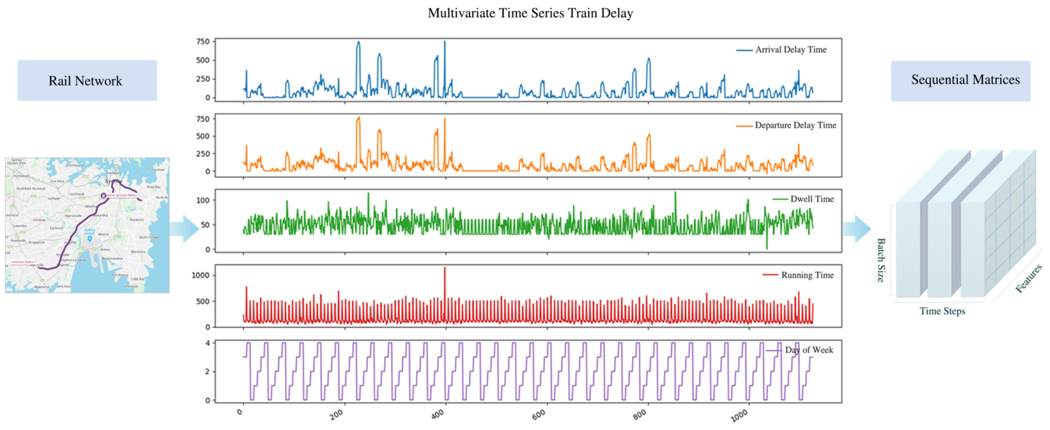
Figure 1. Graphical representation of feature generation process.
Futuretransp 01 00042 g001
Figure 2. LSTM-CPS network topology.
Futuretransp 01 00042 g002
Figure 3. A standard LSTM unit.
Futuretransp 01 00042 g003
Figure 4. Training and validation loss for a running time prediction with MAE as loss function.
Futuretransp 01 00042 g004
Figure 5. RMSE, MAE, MAPE, and training time for running time prediction.
Futuretransp 01 00042 g005
Figure 6. RMSE, MAE, MAPE, and training time for dwell time prediction.
Futuretransp 01 00042 g006
Figure 7. R-squared and Adjusted R-squared.
Futuretransp 01 00042 g007
Table 1. Performance on running time prediction.
ModelRMSE (sec)MAE (sec)MAPE (%)Training Time (sec)
Random Forest148.431107.1562.8251.2
CNN20.015.41114.5838.3
LSTM20.41914.97311.77956.6
Bidirectional-LSTM25.25619.13614.90763.7
CNN-LSTM24.21817.07615.06647.1
GRU-LSTM21.52718.08615.96085.2
Table 2. Performance on dwell time prediction.
ModelRMSE (sec)MAE (sec)MAPE (%)Training Time (sec)
Random Forest13.4189.98023.6881.2
CNN18.12814.49124.0143.8
LSTM16.67012.12518.89717.7
Bidirectional-LSTM15.58611.14717.10724.3
CNN-LSTM14.83710.22915.49819.8
GRU-LSTM14.7179.84414.48029.9
Publisher’s Note: MDPI stays neutral with regard to jurisdictional claims in published maps and institutional affiliations.