Driving Cycles for Estimating Vehicle Emission Levels and Energy Consumption

Abstract

Standard driving cycles (DCs) and real driving emissions (RDE) legislation developed by the European Commission contains significant gaps with regard to quantifying local area vehicle emission levels and fuel consumption (FC). The aim of this paper was to review local DCs for estimating emission levels and FC under laboratory and real-world conditions. This review article has three sections. First, the detailed steps and methodologies applied during the development of these DCs are examined to highlight weaknesses. Next, a comparison is presented of various recent local DCs using the Worldwide Harmonized Light-Duty Test Cycle (WLTC) and FTP75 (Federal Test Procedure) in terms of the main characteristic parameters. Finally, the gap between RDE with laboratory-based and real-world emissions is discussed. The use of a large sample of real data to develop a typical DC for the local area could better reflect vehicle driving patterns on actual roads and offer a better estimation of emissions and consumed energy. The main issue found with most of the local DCs reviewed was a small data sample collected from a small number of vehicles during a short period of time, the lack of separate phases for driving conditions, and the shifting strategy adopted with the chassis dynamometer. On-road emissions measured by the portable emissions measurement system (PEMS) were higher than the laboratory-based measurements. Driving situation outside the boundary conditions of RDE shows higher emissions due to cold temperatures, road grade, similar shares of route, drivers’ dynamic driving conditions, and uncertainty within the PEMS and RDE analysis tools.

1. Introduction

Exhaust emissions from vehicles present a serious risk in urban areas, affecting air quality and human health [1]. Vehicle emissions are influenced by on numerous issues such as driving style, traffic congestion, emission control devices, vehicle performance, fuel quality, and ambient operating conditions [2].

The DC has been defined by various authors as “a series of data points representing speed versus time, and gear selection as a function of time, speed versus distance in a specific region, or a part of a road segment” [3] and “a speed-time profile for a study area within which a vehicle can be idling, accelerating, decelerating, or cruising” [4]. The most important functions of vehicle driving cycles are to determine emission levels and FC [4,5], evaluate vehicle performance [6], estimate driving style [7], and simulate driving circumstances on a laboratory chassis dynamometer (CD) [8], which provides the basis for vehicle design [9]. For electric vehicles, the driving range calculation and state of charge estimation are generally performed on the basis of the standard driving cycle [9].

Several DCs have been developed in different countries to represent local driving conditions. DCs can be legislative or non-legislative [9,10]. Legislative DCs have been established in the US, the European Community, and Japan; FTP75, New European Driving Cycle (NEDC), and JC08 respectively, they have been used for exhaust emissions specification imposed by governments for car emission certification [10]. Non-legislative DCs have been investigated in different countries and cities such as Vadodara [1], Bangalore [5], the Malaysian Urban Driving Cycle (MUDC) [11], Hong Kong [12], Pune [13], Edinburgh [14], Athens [15], Singapore [16], and 11 Chinese cities [17]. Non-legislative cycles have broad application in research for energy conservation and pollution evaluation. All have been employed in research ranging from performance estimation to vehicle design.

Emissions from vehicles are affected by DCs which mainly depend on traffic conditions [15]. Therefore, many research studies have been targeted at developing DCs using recorded real-world driving data encountered in road driving. As DCs vary from city to city and area to area, existing DCs in certain countries may not be suitable to other countries. Researchers strongly agree that the driving characteristics are unique due to different vehicle fleet composition, driving behaviour, and road network topography [18].

The WLTC developed by the UNECE [19] replaced the NEDC for the type of approval testing of light-duty vehicles with the transition to the Euro 6c emission standard in September 2017 [20]. Compared with NEDC, WLTC has a higher maximum velocity, higher acceleration, and lower percentage of vehicle idling time. It also covers a wider range of operating conditions [21], considers more real-world factors [22], and enables best and worst values to be shown in customer information [23]. The WLTP is performed under CD conditions, which cannot take into account weather conditions, traffic situations, and driving style; thus, it is complemented by real driving emissions (RDE) [23]. The FC rate under the China Light-Duty Vehicle Test Cycle (CLTC) shows a 13.5% higher value than WLTC test results [24]. The acceleration and deceleration modes of WLTC show relatively more aggressive driver behaviour due to their large time proportions [25]. Ma et al. (2019), indicate that, in China, fleet average FC for off-peak and peak DCs are 6.6% and 27.8% greater than the average simulated FC of WLTC [26].

The driving cycle developed by the US Environmental Protection Agency (EPA) underwent numerous changes until the end of 2008. It comprises four parts: city driving (FTP75), highway driving (HWFET), aggressive driving (SFTP US06), and the operational air conditioning test (SFTP SC03). The emission value for certification of passenger cars (PCs) and light-duty trucks (GVWR under 3.86 tonnes) is calculated as a weighted composite value of emissions comprising 35% FTP75, 28% US06, and 37% SC03 [27]. For FC, the FTP75 test cycle has a weighting of 55%, and the test of the HWFET 45% [28]. The US cycles are closer to real-world driving style behaviour [29]. It is accepted by many that the shortfall between certified and on-road fuel consumption has increased in US passenger vehicles [30]. Seers et al. (2015) revealed at least a 31% increase in FC over FTP75 for utility vehicles [31].

The Japanese driving cycle JC08 [32] has been used for emission certification of PCs and light-duty trucks since 2011 [33]. JC08 is highly transient with a minimum cruising time and long idling period, with a cold start weighted at 25% and a hot start at 75% [27].

The CD and emission model software are used most to determine vehicle emission factors. However, in recent years, researchers have found a significant gap in emissions reported using the above two methods. Measuring vehicular emissions on a CD involves driving a vehicle through a predetermined DC [6,19] by a human driver, with a device known as a driver’s aid informing the driver how to drive the vehicle, including speed tolerances around the target speed trace [28]. During this test, the exhaust flow rate is continuously monitored, and the exhaust gas is collected in sample bags for subsequent analysis of content and concentration after dilution with ambient air. A constant volume sampler (CVS) system based on a CD is displayed in Figure 1 [2].

COPERT 5 software overestimated CO by 131.9% and underestimated NO_X by 63%, compared with the on-road measurement [34]. COPERT also estimated that FC was 9% lower than the experimental data due to COPERT being an average based numeric model [35]. Amin et al. (2018) compared on-road emission factors in Mashhad, Iran with those obtained from the international vehicle emission (IVE) model. On-road emissions of CO, HC, NO_X, and CO₂ were 9.45, 0.06, 2.05, and 392 g/km, respectively, and the simulated emissions by the IVE model of CO, VOC, NO_X, and CO₂ were 100.52, 0.43, 1.12, and 335.06 g/km, respectively [36]. Comparing COPERT with PHEM software, the relative deviations were −32.1% for FC and −24.4% for NO_X emissions [37].

Several researchers developed the local DCs, but these need to be examined in relation to the quality and quantity of raw driving data. Based on the reviewed papers, there are different DC construction methods, data clustering, and cycle assessment parameters. The aim of this paper is to explore the detailed methods applied in each step of the DC development and compare the recently developed local DCS with standard DCs such as WLTC and FTP75. This will help to guide the selection of methods that can be applied for DC development and assessment. This review paper has three sections. First, the detailed steps and methodologies applied during the development of the DCs are examined to highlight their weaknesses. Next, a comparison of various recent local DCs with WLTC and FTP75 are presented in relation to the main characteristic parameters. Finally, the gap between RDE with laboratory-based emissions measurement and real-world emissions is discussed. Recent papers were selected whose full text could be accessed and that present local DCs with values of the main cycle assessment parameters.

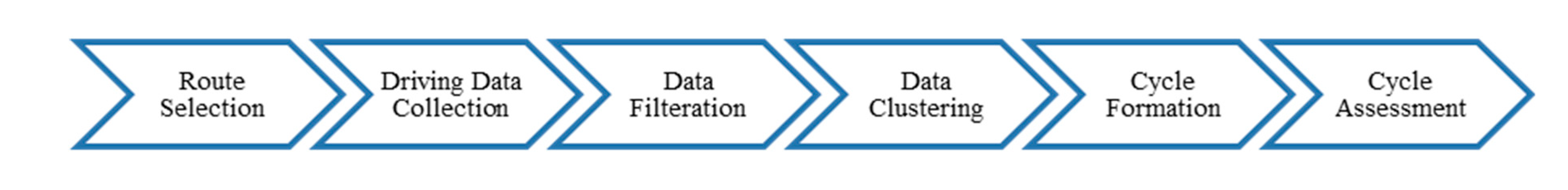
2. Driving Cycle Development Process

As shown in Figure 2, there are six common major steps in the development of vehicles DCs.

2.1. Route Selection

Traffic congestion in an urban environment is believed to vary depending on the route and time, with heavier traffic congestion expected during normal weekdays and at peak times compared with weekends or public holidays and off-peak times [11]. From the actual road network of the study area, representative routes should be selected, considering traffic flow conditions affected by road type, topography, intersections, population density, gradient, and weather conditions [38]. To select the routes, actual situations that occur along each route must be identified and ascertained [6]. The chosen routes require the following features: (1) a high traffic volume, (2) connecting major centres of population, (3) high emissions on the transit route, (4) various squares and intersections, and (5) access to public transport systems [36].

Route selection is an essential process when developing DC. Researchers typically use their knowledge and understanding of local conditions to select the sample routes [39]. This method of route selection may cause a selection bias if the relevant factors are not considered. Peng et al. (2019) collected driving data from seven vehicles without route planning for 20 weeks in Fuzhou city [40], while Anida (2019) simply selected the five most frequent routes [41]. To develop the Mashhad DC, two major routes were chosen that had the same starting point and destination (Azadi square—Barq square), both 15 km in length. The reason for their selection was that Azadi and Barq squares connect East–West and North–South Mashhad and have the highest traffic volume [36]. To develop the MUDC, five routes were selected based on observations, and the test was conducted on weekdays without public holidays, from Monday to Friday, during peak hours from 07:30 to 11:30, thus encompassing a mixture of halt traffic, slow traffic, smooth traffic, and highway driving within the area of study [11].

Some researchers have developed a methodology or an approach for selecting the most representative routes. Zhao et al. (2018) analysed the overall topological structure of urban roads in Xi’an using ArcGIS software, established monitoring points on various types of selected sample roads, and then investigated traffic flow to identify peak and off-peak times, before ultimately deciding on the length of each test route [9]. Galgamuwa et al. (2016) developed an economic approach to collect speed–time data in Colombo, Sri Lanka by considering vehicle travel activity patterns throughout the city using origin-destination survey data. The selected routes were divided into links using nodes or physical junctions to minimise segment length, then divided again into five groups according to daily traffic to identify the proper weightage for these routes. Traffic flow variation in a typical day was divided into seven segments with noticeable variations, and finally, a route with the highest daily traffic within the group was selected as a point estimator to represent each group in order to avoid underestimation [42].

During the development of the Ljubljana urban DC, the path of vehicles was not predetermined. Vehicles were allowed to travel randomly according to travellers’ needs. The study authors then used a geographical information system (GIS) to identify data for the study area. Out of a total of 6,825,444 collected records, GIS analysis identified 416,471 records as the data within the analysed area that provided the database for further procedures [43].

In the Delhi DC, the study authors classified traffic as congested, semi-urban, urban, and extra urban conditions [44]. In CLTC, traffic conditions were classified based on the vehicle speed phase: a low, medium, and high-speed phase with the threshold of 60, 80, and 120 km/h, respectively, based on the weighting factors of the different speed phases. Finally, the values obtained for a low, medium, and high-speed phase were 674, 693, and 433 s, respectively [24]. The most common steps needed for a representative route selection are:

• determining the peak ratio of peak hour;
• preparing criteria for categorizing routes as urban, rural, or highway;
• ranking the routes based on the level of service (LOS);
• selecting and determining the sample route length for urban roads, rural roads, and highways.

2.2. Driving Data Collection

From the fleet in the study area, representative vehicles should be selected and equipped with instruments that collect and store driving activity data from the selected routes. Three methods have commonly been used to collect driving data [11,36]:

• The chase-car method. Here, a vehicle fitted with a data collection device is allowed to follow the target vehicle. With this technique, the vehicle to be followed is randomly selected, and then, the operations of this vehicle are replicated at a distance. If the selected vehicle drives out of the area of study, the chase car immediately chooses a new vehicle to follow. At the end of each route, the logged data are briefly reviewed to ensure there are no errors before proceeding to the next route [11]. This approach to data collection can record only a specific section of the driver’s trip [45], can omit details of the entire trip, and is applicable for areas with minimal and smooth traffic flows [42]. With this technique, two methods are available for collecting data from target vehicles: laser technology and unlock data [45].
• The on-board measurement technique: to use this technique, instruments are fitted on target vehicles to record the speed data as they travel along the predetermined routes. This can be used in areas with high and aggressive traffic flow [42].
• The hybrid technique: this is a combination of on-board measurement and circular driving, in which a test vehicle with the instrument travels along the selected routes during peak and off-peak hours several times [9].

For the accurate development of DCs, a large sample of representative driving data is required [43]. Among the current technologies, GPS and an on-board diagnostics (OBD) interface are the most common instruments for the collection of driving data.

GPS: provides data on a vehicle’s velocity, time, date, latitude, longitude, and altitude. Galgamuwa et al. (2016) used the on-board measurement method with five GPS devices for data collection in the study area, collecting data on 78 trips at one second intervals [42]. GPS-based data collection has the advantages of being small and easy to carry on vehicles, device installation and operation not affecting the operation of a vehicle, good signal reception, bulk data storage, and being a high frequency data acquisition system [46]. A similar approach was taken by [25,41,47,48,49] for data collection using GPS.

OBD interface: provides data on engine RPM and load, vehicle speed, and fuel flow rate. It has a better data quality and greater accuracy than GPS-derived speed data [16]. Various devices are available for connecting to the OBD II port; some are car chip devices [8], and others are ELM TM Bluetooth devices [38].

Zhao et al. (2018) used a hybrid method to record driving data, with speed–time data recorded by OBD being used to enhance abnormal GPS data [9]. Lipar et al. (2016) used an on-board measurement technique that included an OBD II interface, a GPRS/GMS module, and a GPS to record driving data [43]. Liu et al.’s (2021) data acquisition equipment included vehicle and engine speeds sampled from the OBD interface and longitude and latitude obtained by GPS devices [50].

A comparison of raw data gathered for local DCs and WLTC is presented in

Table 1. Comparison of raw data gathered for developed DCs and WLTC.

Driving Cycle	No. of Vehicles	Data Collection Duration	Pathway Selection	Route Type/LOS	Collected Raw Data	Duration of DC	% of Cycle Duration to Raw Data
LJURBAN [43]	19	6 months	Not predetermined	-	416,471 s	1587 s	0.38
Mashhad [36]	1	2 weeks	Predetermined	Two major routes	25,500 s	1020 s	4
MURDC [51]	1	-	Predetermined	Normal and highway	224 MTs	16 MTs 1500 s	7.14
Baqubah [8]	1	7 days	Predetermined	From different routes in the city	33,512 s 200 km	1052 s 6.33 km	3.14/3.16
Basrah DC [52]	1	5 weeks	Predetermined (4 paths)	light and peak traffic conditions	20,912 s	1041 s 6.273 km	4.98
CLTC [24]	3767	1 year	Not predetermined	Urban, rural and motorway	32 million km	14.48 km 1800 s	4.5 × 10−5
Tianjin [50]	5	2 months	Predetermined	Main, secondary, branch roads and Expressways	165,166 s	1800	1.09
Zhengzhou [53]	-	2 weeks	Predetermined (2 routes)	All level of roads	600,000 s	1184	0.2
Nanjing [25]	1	1 month	Predetermined 5 major routes	Considered also expressways	46,569 s 77.1 km	1172	2.52
TMC [54]	15	8 months	Predetermined	Urban, extra urban and mixed extra urban and urban in flat road	54,867 s 72 km	6000 s	10.93
Bangalore [5]	1	3 weekdays	Predetermined	6 routes	18 h 250 km	2088 s 9.4 km	3.22/3.76
MUDC [11]	1	-	Predetermined	5 routes	367 MTs	1138 s
Colombo [42]	5	-	Predetermined	Both trip type	175 h	1200 s	0.19
WLTC [55]			Not predetermined	Urban, rural and motorway	765,000 km	23.21 km 1800 s	3.03 × 10−3

.

As presented in Table 1, one vehicle was used in data collection for the development of the Mashhad, Baqubah, and Basra DCs, etc., but for the development of CLTC, 32 million km of raw data were collected from 3767 vehicles, of which 34% of vehicles were hybrid and electric vehicles. In CLTC, the driving data of traditional and electric vehicles were combined, which is one of its weaknesses. Numerous researchers have developed a separate DC for hybrid and electric vehicles. To obtain the most representative DC, it is better to consider peak, off-peak, and weekend-driving situations during data collection. To evaluate the representativeness of the collected sample size of local DCs, this study introduced of the percentage of developed cycle duration to the size of the raw data collected. The data collection duration showed high variation between the compared DCs of between three days and one year. Regarding the amount of raw driving data collected, CLTC involved the largest and broadest data collection in the history of DC development. The percentage of local DCs was between 0.19 and 10.93, except for CLTC, which is very high compared with WLTC and CLTC at 3.03 × 10⁻³ and 4.5 × 10⁻⁵, respectively. This clearly indicates that local DCs are less representative. As observed from the local DCs reviewed, the reason for the collection of the small amount of driving data with a few vehicles and predetermined route selection is to minimise the budget required for data collection.

2.3. Raw Data Filtration

There are several errors in the collected data samples from GPS; thus, a data filtration process is required [56,57]. Based on the reviewed papers, many researchers skipped this step. However, a few of them applied and proposed a GPS data filtration process.

Nguyen and Bui (2020) proposed a GPS filtering process consisting of nine steps. Developing a MATLAB code to detect and repair errors in the GPS data, in the last steps of the filtration process, a modified Kalman filter process was applied to de-noise and smooth final signals [58].

Duran and Earleywine (2018) applied seven logic-based filters for the filtration process to remove duplicated records and negative differential time steps, replace outlying high/low-speed values, remove zero-speed signal drift when the vehicle stopped, replace false zero-speed records, amend gaps in data, repair outlying acceleration or deceleration values, and denoise and smooth final signals using the Savitzky–Golay filter technique [59].

Huertas et al. (2018) disregarded trip data that were missing typical values with less than 90% of available data. Rather than fixing missing values, they ignored the data [60].

2.4. Data Clustering

The filtered data were clustered into different groups, with each group designed to represent different driving characteristics and congestion levels. Clustering is applied for gathering micro-trips with similar speed–acceleration values [60]. Clustering is an appropriate approach for grouping the large number of micro-trips into a smaller number of micro-trips, and the candidate DC is generated by chaining micro-trips from an individual cluster [1].

K-means clustering is the simplest and most popular algorithm used for grouping enormous data sets [1,38]. K-means algorithms were applied by [1,41,49] for clustering micro-trips. He (2020) applied the mean shift clustering method to overcome the problems of K-means clustering [61].

Three clusters were mostly used to reflect the level of traffic congestion level: low, medium, and high speed. In the development of the Kuala Terengganu city DC, data were clustered into three clusters: clear traffic conditions, medium traffic conditions, and congested traffic conditions [41]. During the development of Beijing’s DC, the recurrent neural network (RNN) was applied for the DC classification task. An RNN is formed by a variable’s number of connected identical RNN cells, where each cell utilises the state yielded by the previous one [56].

Driving Modes

The most common driving modes were idle, cruising, acceleration, and deceleration [57]. In the RDE regulation, acceleration is defined as a > 0.1 m/s², but there were slight variations in values between different researchers to categorise driving modes, as shown in

Table 2. Driving mode classification.

References	Driving Modes
	Idle	Cruising	Acceleration	Deceleration
Lairenlakpam et al. (2018) [57]	V < 1.389 m/s and −0.1389 < a < 0.1389 m/s2	V ≥ 1.389 m/s and −0.1389 < a < 0.1389 m/s2	a ≥ 0.1389 m/s2	a ≤ −0.1389 m/s2
Yang et al. (2019) [25]	V < 0.278 m/s and −0.14 < a < 0.14 m/s2	V ≥ 0.278 m/s and −0.14 < a < 0.14 m/s2	a > 0.14 m/s2	a < −0.14 m/s2
Chauhan et al. (2020) [1]	V < 1.389 m/s and −0.1 m/s2 < a < 0.1 m/s2	-	a >0.1 m/s2	a < −0.1 m/s2
Liu et al. (2020) [24]	V < 0.1389 m/s and a < 0.15 m/s2	V ≥ 0.1389 m/s and a < 0.15 m/s2	a ≥ 0.15 m/s2	a ≤ −0.15 m/s2

.

2.5. Decide DC Length

DC length is very important for proper representativeness and better measurement of emission level and FC testing in the CD. It should not take too long or be too complex to conduct tests in a CD. There should be an agreement between the representative DC and its responsiveness to the CD [44].

The length of CLTC was determined based on the length of the low-, medium-, and high-speed phases, which was determined based on the weighting factors of the different speed phases. The low-, medium-, and high-speed phases had values of 674, 693, and 433 s, respectively [24]. In Delhi’s DC, the length was set at a duration of 1500 s by considering the trends of legislative DCs [44]. Similarly, Malaysia’s urban road cycle was 1500 s, with the authors reporting that this length was sufficient for the experimental works in the CD laboratory test [51].

2.6. Driving Cycle Formation

The method of cycle formation varies with the use of the DC. The DC can be used to estimate emission inventories and FC or for traffic engineering purposes [3]. Previously, there were four major DC formation methods: micro-trip based, segment based, pattern classification, and modal cycle formation [40,62,63]. Recently, Huertas et al. (2018) developed a new approach called the fuel-based method. Each method has unique features to represent its intended purpose [60].

2.6.1. Micro-Trip Based Cycle Construction

The duration between the start of the idle period and the next moment of the idling period is defined as a micro-trip [40], including the leading idle period [3]. In this method, the cycle is constructed based on the driving data divided into different bins according to average speeds when target population parameters are met. Finally, a set of micro-trips is selected and spliced together to form a candidate DC [3]. The two most common methods are quasi-random selection [60] and the best incremental method [23]. However, for the combination of micro-trips, Mahayadin (2018) applied Chi-squared analysis for the speed-acceleration frequency distribution (SAFD) as a measure of the difference between the selected micro-trips combination and the whole database, ultimately selecting the combination with the lowest Chi-squared value [51].

The Vadodara [1], Ludhiana [49], Bangkok [64], Hong Kong [65], Pune [13], and CLTC [24] driving cycles were developed using the micro-trip-based cycle construction method. The advantages and disadvantages of the micro-trip methods are presented in

Table 3. Advantages and disadvantages of driving cycle construction methods.

Method	Advantages	Disadvantages
Micro-trip	A good representation of FC and emissions [66]. Covers each stop–go condition that happens due to traffic congestion [3]. A cycle is generated based on real driving data [3].	The starts and ends of micro-trips are specific speed, acceleration and duration [67]. Not possible to differentiate micro-trips by different types of levels of services (LOS) [3]. It is repeatable but not reproducible because it is stochastic in nature [68].
Segment-based	Considered LOS [67]. The cycle starts and ends at any speed [4]. Suitable for traffic engineering purposes [3]. Suitable for expressways [3].	Chaining the trip segments into a DC requires the speed and acceleration between two consecutive connection points to be matched [4,38]. Not suitable for emission and FC estimation [3].
Pattern-based		Not directly related to emissions-related DC, highly statistics-based, requires more information to divide collected data into kinematics sequences and to classify the route [69].
Markov chain	Driving patterns are divided into four driving modes. It represents the actual traffic condition because to chain the modal bins it uses the possibility of the occurrence of each mode on the road [3].	If the traffic behaviour of the road is smooth, then it is possible that the occurrence matrix has some gaps, or the duration of the modal event is much longer than the total length of the cycle [3].
Fuel-based	Fuel-based DCs are almost the same as the measured FC in flat roads [60]. It is repeatable and reproducible [70,71]	The duration of the selected DC cannot be controlled [70,71].

. To minimise the limitations of the micro-trip method, Kiran and Verma (2018) proposed a new method called the trip segment method, along with an algorithm to extract those units from the given data [5].

2.6.2. Segment Based Cycle Formation

In this approach, the roadway type or LOS is considered, when selecting a trip segment instead of adjacent stops [67]. As a result, the trip segment can represent the actual traffic conditions and characteristics of the road based on LOS [4,68]. Therefore, when chaining the trip segments into the DC, it is necessary to match the speed and acceleration between two consecutive connecting points [4,70]. This method is suit-able for a DC for traffic engineering purposes and expressways, because there are no adjacent stops between the origin and destination [3]. The Australian Composite Urban Emission Drive Cycle (CUEDC) was developed using this method [72].

2.6.3. Pattern Classification

In this method, DCs are constructed based on the statistical method by a random selection of kinematic sequences from segmented activity classes considering the probability and events of kinematic sequences [71]. ARTEMIS driving cycles were developed using this method [3].

2.6.4. Modal/Markov Chain Approach

In this method, real-world driving data patterns are divided into acceleration, deceleration, cruising, and idling components based on Markov chain theory which assumes that the likelihood of a particular modal event depends only on the previous modal event [3]. The “wavelet theory” is applied to analyse the different frequency components of driving data. It is applied to analyse the components of velocity and decomposing cycle formation into several signals with different frequencies [72]. Researchers in [42,48,53,66] applied the modal cycle construction method, which is the Markov chain approach.

2.6.5. Fuel-Based Approach

The instant vehicle fuel flow rate is measured through the engine control unit (ECU), providing the opportunity to construct a driving cycle based on the FC principle. In this approach, the average specific fuel consumption (SFC) of the trips sampled is computed. Then, the trip with the SFC closest to the average SFC is selected as a representative DC [59,73].

Huertas et al. (2018) suggest a method to develop a local DC that uses FC as a criterion. Data were collected from a fleet of 15 vehicles of similar technology using the OBD interface provided by the engine manufacturer to read, report, and store instantaneous engine FC at a 1 HZ sampling period and with GPS to monitor the position, altitude, and speed of the vehicle as a function of time during eight months of normal operation in four regions with diverse topography and roads with diverse LOS. The results confirmed that characteristics parameters and SAPD of the fuel-based DCs were almost the same as the measured FC on flat roads [60].

2.7. Conformity Assessment

A number of candidate cycles can be obtained from different run series of similar raw driving data. Thus, the most representative candidate cycle that confirms the best cycle in relation to real-world driving data should be determined. The conformity evaluation of the candidate cycles with real-world driving data is analysed based on:

• speed acceleration frequency distribution (SAFD)—the smallest SAFD_diff value is selected as the best DC [1,47];
• performance value (PV) [49];
• sum squared difference (SSD) [49];
• correlation factor (CF)—CF value close to one can be selected as the representative DC of the route [38];
• Chi-squared—the combination of short trips with the smallest chi-squared value was selected for CLTC [24];
• Euclidean distance—the smallest Euclidean distance for each DC derived should be chosen [52];
• relative error—an error of 5% is considered acceptable for each parameter, and if the error is more than 5%, develop a DC again by a random combination of micro-trips, continuing the process until the error rate is less than 5% [1].

2.8. Assessment of the Developed DC

The developed DC should be evaluated to ensure that it represents the on-road data collected and can be compared with the standard DC to specify its deviation. Characteristics parameters are used in cycle assessment, which ensures that the developed cycle correctly reflects the real driving pattern [48]. Researchers have used different parameters to compare developed DCs with collected real data and other DCs. There are more than 58 parameters.

From the reviewed papers, many of them used a set of cycle assessment parameters, following the experience of previous studies but without providing strong justifications for this. However, to select target parameters that significantly affect emission levels and FC, Nguyen (2019) applied the hierarchical agglomerative clustering (HAC) method to determine a minimum subset of representative variables from 33 variables, ultimately selecting the 14 that were most representative [48]. Ericsson (2001) used factorial analysis to reduce the initial 62 parameters to 16, nine of which were found to have a considerable effect on emissions [74]. Lee and Filipi (2011) used statistical regression analysis to determine the significance of each parameter for the representation of the response of DCs and found eight of the 27 variables to be significant variables for assessing the DC [75].

The emission rates of CO₂, CO, and NO_X are more sensitive to speed and acceleration, decreasing with the increase in absolute value of acceleration in low-speed and medium-speed zones and rising with the increase in speed and acceleration in high-speed zones [25]. The emission rates of CO and NO_X reach a peak when speed and acceleration are at their maximum, but the maximum HC rate is often found in the medium-speed and high-acceleration zone. When tested in local DC, the highest emission rates of CO₂, CO, and NO_X appeared in acceleration mode, and the lowest values appeared in idling mode [25]. However, with modern vehicles and after treatment devices, a direct correlation is not always seen [76].

Table 4. DC characteristic parameters.

Category	Parameters	Units	[49]	[11]	[48]	[52]	[41]	[53]	[54]	[58]	[51]	[50]	[43]
			LuDC	MUDC	HB DC	BCC DC	KT DC	ZDC	TMC	HDC	MURDC	TDC	LJDC
Cycle distance and time related	CL	km		5.86	18.32	6.27	10.07	4.92		18.32	13.29	10.31	10.19
	CT	s		1138	3936	1041	1089	1184		3936	1500	1800	1587
Driving mode related	% of tdriv	%		63.18									77.5
	Pc	%	2.39		14.1		4.68	14.49	29.3	3.6	61.73		22.55
	Pa	%	51	32.43	34.17		45.78	33.32	27.2	46.90	10.13		27.73
	Pd	%	41.17	30.76	32.70		42.84	28.78	23.7	48.79	8.73		28.23
	Pi	%	5.40	36.82	7.62		6.7	22.93	19.3	3.37	19.4	26.7	22.5
	Pcr	%			11.41
	tacc	s			1345								440
	tdec	s			1287								448
	tcru	s			555								342
	tcre	s			449
	tidl	s		419	300								357
	tdriv	s											1230
Vehicle speed related	Vtrip	km/h		20.6	16.76		36.27			17.38	37.17		29
	Vavg	km/h	24.83	21	18.14	21.63	33.27	14.96	11.2	16.67	31.89	20.62	22.5
	SD of V	km/h		21.4	10.52			13.56	9.7	10.71		0.78	18.57
	75th–25th% of V	km/h											35
	95th% of V	km/h			33					36.4
	Vmax	km/h		91	44	63.62		49.63	28.4	46.3		83.4	70
Acceleration related	aavg	m/s2		0.53	0.5		0.53		0.4	0.46	0.75	0.47	0.83
	davg	m/s2			−0.52		0.56		−0.5	−0.44	−0.89		−0.77
	aSD	m/s2			0.49			0.7	0.2	0.06		0.02	0.61
	dSD								0.4	0.05
	a95th	m/s2			1.11
	d95th	m/s2			−1.11
	No. of a			79									151
	No. of ‘a’ per km	/km		13.48					7.4				14.82
	amax	m/s2			3.06	2.66		4.031	1.6	3.85		2.43
	dmax	m/s2			−2.78	−3.09		−5.4	−2.1	−3.39
Stop related	No. of stops			18	21	7							21
	Stops per km	/km		3.07	1.15	0.87							2.08
	Avg. distance between stops	m											485.19
	PKE	m/s2			0.34				241.3				0.51
	RMSA	m/s2			0.49		0.72		0.4
Slope related	imax	-						4.79
	imin	-						−3.4
	iavg	-						−0.23

LuDC is the Ludhiana driving cycle, HBDC is the Hanoi driving cycle, KTDC is the Kuala Terengganu driving cycle, ZDC is the Zhengzhou driving cycle, TMC is the Toluca-Mexico city driving cycle, HDC is the Hanoi driving cycle, MURDC is the Malaysia’s urban road driving cycle, TDC is the Tianjin driving cycle, LJDC is the LJURBAN driving cycle, C_L is the driving cycle length, C_T is the driving cycle duration, t_driv is the driving time, P_a is the percentage of acceleration time, P_d is the percentage of deceleration time, P_i is the percentage of idle time, P_c is the percentage of cruise time, P_cr is the percentage of creeping mode, t_acc is the acceleration time, t_dec is the deceleration time, t_cru is the cruising time, t_cre is creeping time, t_idl is the idling time, V_trip is average trip speed, SD is the standard deviation, V is the vehicle speed, V_avg is the average driving/vehicle speed, V_max is the maximum vehicle speed, a_avg is the average acceleration, d_avg is the average deceleration, a_95th is the 95th percentage of acceleration, d_95th is the 95th percentage of deceleration, PKE is the positive kinetic energy, RMSA is the rroot mean square of acceleration, VSP_max is the maximum specific power, i_max is the maximum slope, i_min is the minimum slope, and i_avg is the average slope.

offers a simple portrayal of the most frequently used parameters.

2.9. Comparison of Driving Cycles

A comparison of the cycle parameters of the TDC [50], CLTC [24], HDC [58], LuDC [49], Vadodara [1], ZDC [53], HBDC [48], KTDC [41], Nanjing [25], TMC [54], Bangalore [5], MURDC [51], Mashhad (MDC) [36], MUDC [11], Baqubah [8], Colombo [42], LJDC [43], and Toronto Waterfront Area (TWFA) [77] DCs developed from 2016 to 2021 with WLTC and FTP75 are presented in

Table 5. Comparison of local and standard DCs.

Name of DC	Year	Vavg (km/h)	Vmax (km/h)	% of Pi	% of PC	% of Pa	% of Pd	CL (Km)	CT (Sec)	Considered Routes
TDC [50]	2021	20.62	83.4	26.7				10.31	1800	Expressways, main roads, secondary roads, and branch road
CLTC [24]	2020	28.96	114	22.11	22.83	28.61	26.4	14.48	1800	Urban, rural and motorway
HDC [58]	2020	16.67	46.97	7.62	14.1	34.17	32.7	18.32	3936	Urban area
ZDC [53]	2020	14.96	49.63	22.93	14.97	33.32	28.8	4.92	1184	Not clear but heterogeneous traffic condition was considered
HBDC [48]	2019	18.14	44	7.62	14.1	34.17	32.7	18.32	3936	Inner-city (circular, radial, and straight route types)
KTDC [41]	2019	33.27	65	6.7	4.68	45.78	42.8	10.07	1089	Not clear
Nanjing [25]	2019	30.73	85.65	20	30	27	23	10	1172	Expressways, arterial roads, secondary trunk roads, and branch roads
TMC [54]	2019	11.2	28.4	19.3	29.7	27.2	23.7	18.67	6000	Urban, extra-urban, and mixed urban and extra-urban of medium traffic flow
Bangalore [5]	2018	20.71	65.17	21.75	13.56	34.74	30	9.4	2088	Not including motorways
MURDC [51]	2018	31.89	90	19.4	61.73	10.13	8.73	13.29	1500	Urban, highway
MDC [36]	2018	20.41	60	21.75	3.22	37.34	37.69	5.78	1020	Arterial road
MUDC [11]	2018	21	91	36.82	-	32.43	30.8	5.86	1138	Standstill, slow, smooth, and highway driving
Baqubah [8]	2017	21.63	68	25.56	0	50.33	48.5	6.33	1052	Not clear
Colombo [42]	2016	20.3	58	20.5	12.75	36.1	30.7	6.77	1200	Considered different routes based on daily traffic conditions
LJDC [43]	2016	22.5	70	22.5	21.55	27.73	28.2	10.19	1587	Not considering motorway
TWFA [77]	2015	18.4		17.1	3	43.8	36.1	9.2	1800	Major arterials
WLTC * [24]		46.42	131	12.7	27.8	30.9	28.6	23.21	1800	Urban, rural, and motorway
FTP75 * [24]		33.9	90.16	17.2	24.7	31.1	27.1	17.68	1874	Cold, stabilisation, and hot phase
JC 08 * [27]		24.4	81.6	28.74	1.5	36.13	33.64	8.16	1204	Including motorway, but it is shorter (154 s)
ARTEMIS [36]		59.2	150.4	9.64	16.19	38.84	35.32	51.69	3143	URM 150 (urban, rural, and motorway)
NIER−09 * [78]		34.1	70.9	11.7	0	43.4	44.9	8.74	926
CUEDC Petrol * [27]		38.95	94	20.42	25.26	26.82	27.49	19.44	1797	Congested, residential, arterial, and freeway

(*) Indicates standard driving cycle, CUEDC (Composite Urban Emissions Drive Cycle), ARTEMIS (Assessment and Reliability of Transport Emission Models and Inventory System), NIER (National Institute of Environmental Research).

.

As shown in Table 5, Ludhiana and Kuala Terengganu DCs have lower idle ratios of 5.4% and 6.7%, respectively, thus indicating normal traffic conditions, and Vadodara DC and MUDC have higher idle ratios of 39.2% and 36.82%, respectively, compared with other DCs, thus indicating greater traffic congestion, and these cities having numerous signalised intersections within a short distance. Ludhiana and Baqubah have higher acceleration ratios of 50.99% and 50.33%, respectively, and Malaysia’s urban road cycle has a lower acceleration ratio of 10.13% compared with the other cycles. The statistical analysis of the compared local driving cycles showed that the mean of idle, cruising, acceleration, and deceleration proportions were 19.77 ± 7.89%, 17.35 ± 16.07%, 33.25 ± 9.74%, and 30.22 ± 9.27%, respectively. It was observed that the percentage acceleration and percentage deceleration were high for most local DCs compared with the standard DCs, meaning that vehicles release more emissions if the local DC is used in CD compared with standard DC. The percentages of cruise and idle were observed to be less than others.

Regarding vehicle velocity, as shown in Table 5, the average and maximum speed of WLTC is 46.42 km/h and 131 km/h, which is very different from other local DCs. The V_max of CLTC is highest at 114 km/h, compared with other local DCs, thus indicating better road infrastructures in China, while for other local DCs, the lowest maximum speed of less than 100 km/h indicates the absence of motorways during the data collection period or a lack of such roadways. From local DCs, the V_avg of the KTDC has the highest speed of 33.27 km/h, with MURC next at 31.89 km/h, thus indicating lower traffic congestion. The statistical analysis of the compared local DCs showed that the means of V_avg and V_max were 22.06 ± 6.43 km/h and 68.40 ± 23.66 km/h, respectively. The mean of the average speed of local DCs was observed to be less than standard DCs, except for JC08.

Table 5 shows that the ARTEMIS, WLTC, and TMC are longer than other cycles, at 51.687 km, 23.21 km, and 18.667 km, respectively, and the shortest cycle is MUDC at 5.86 km. Regarding the cycle duration shown in Table 5, Toluca–Mexico City and Hanoi cycles have the highest cycle time at 100 min and 65.6 min, respectively. The mean cycle length of compared local DCs was 11.07 ± 4.59 km, which is less than WLTC, FTP75, ARTEMIS, and CUEDC, indicating that, on average, the local DC length is shorter than the standard DCs.

3. Comparison of RDE Tests with Laboratory-Based and Real-World Emissions

Since 2017, European emission regulations have had an element of legal homologation [79] that requires new passenger vehicles to undergo emission testing on public roads during the certification process [80]. The European Commission (EC) has approved a RDE test to minimize the gap between manufacturer-reported emissions and those emitted on the road [80,81]. PEMS is used for second-by-second measurement of CO/CO₂, NO/NO₂, and particle number (PN) concentrations in the exhaust gas of vehicles under real driving conditions [23,82,83] and simultaneously records the vehicle-related parameters and environmental conditions, such as location, velocity, altitude, and temperature [80]. RDE, which was introduced in European Union legislation, has four sequential regulatory packages: RDE 1 (EU Regulation 2016/427), RDE2 (EU Regulation 2016/646), RDE3 (EU Regulation 2017/1154), and RDE4 (EU Regulation 2018/1832) [84].

Conducting emission tests on a chassis dynamometer (CD) is standard practice for comparing the vehicle’s emissions and verifying whether they remain under the emission limit, as per standards. However, CD tests suffer from shortcomings associated with its non-representativeness of actual on-road driving conditions. Comparison of RDE with laboratory-based cycles (WLTC, FTP75, and CADC) is presented in Table 6.

As indicated in Table 6, the RDE of CO₂ is 3–41% higher than WLTC, except for the results reported by [85,86]. RDE of NO_X is 10–326% higher than the laboratory-based DCs, except for the tests conducted in Beijing and Xiamen. Similarly, the real-world emissions of CO and HC also show an increasing trend compared with laboratory-based emissions measurements. Based on the reviewed articles, on-road emissions and FC are significantly higher than the values reported using CD due to drivers’ aggressiveness, varying local weather conditions, traffic conditions, gradients, etc. The main problem with RDE is that it is not repeatable, compared with laboratory tests. The EU RDE test procedure does not include congested traffic conditions.

Table 6. Comparison of RDE with laboratory-based cycles (WLTC, FTP75, and CADC).

DC	Year	Methods Applied or Source of Sample Data	Country/City of RDE Data	Vehicle Category	Laboratory-Based Emissions Level (g/km)	On-Road Emissions Level (g/km)	Difference	FC	References
WLTC	2020	WLTP and RDE	Gothenburg, Sweden	Diesel and gasoline vehicles	143 for CO2 136 for CO2	148 for CO2 151 for CO2	↑3%CO2 for CI vehicles ↑11% CO2 for SI vehicles		[87]
WLTC	2020	WLTP and RDE	NM	Euro 6b diesel	-	-	-	↑18.03%	[88]
WLTC	2020	Real-world data from the consumer website (Spritmonitor.de)	German	WLTP type approved vehicle (2018)	NM	NM	↑14% CO2	↑14%	[89]
FTP75, HWFET	2020	FTP, HWFET, and US06, and Canadian 5-mode on-road driving cycle	Canada	Gasoline and Diesel LDVs	<0.0435 FTP limit of NOX	0.061–0.326 for NOX	1.4–7.5 times FTP NOX limit	↑22%	[87]
WLTC	2019	WLTP and RDE	Lombardy	Euro 6d-temp diesel (DOC + DPF + SCR)	146.31 for CO2	165.33 for CO2 0.282 for NOX 0.0197 for CO	↑13% CO2		[84]
WLTC	2019	WLTP and on-road testing	Thessaloniki, Greece	Euro 6b diesel (DOC + DPF + EGR)	CO2 close enough to the RDE CO2 levels	NOX are 3 times higher than WLTP level	↓50–100% CO2 and ↑300 for NOX		[86]
Standard road speed	2019	On-road and CD tests	Warsaw	Ford focus PV	229 for CO2 6.9 for CO 1.23 for NOX 1.04 for HC	242 for CO2 7.9 for CO 1.17 for NOX 0.68 for HC	↑5.4% CO2 ↑12.6% CO ↓5.12% NOX ↓50.72% HC		[90]
CADC	2019	CADC and on-road testing	Thessaloniki, Greece	Euro 6b diesel (DOC + DPF + EGR)	NOX levels are close to the levels of the RDE test		NOX levels are close to the levels of the RDE test		[86]
MIDC	2018	MIDC and the average real-world emissions of the three routes	Dehradun city, India	Gasoline (TWC)	216.83 for CO2 0.977 for CO 0.008 for THC 0.011 for NOX	263.35 for CO2 2.03 for CO 0.021 for THC 0.025 for NOX	↑1.12–1.39 times for CO2 ↑1.35–2.39 times for CO, ↑2.17–5.0 times for THC ↑2.04–2.32 times for NOX, and	↑18.4%	[57]
WLTC	2018	WLTP and pre-recorded RDE cycle under lab-RDE cycle	Italy	Euro 6 gasoline (TWC) and diesel (DOC + DPF + NS)	NC	NC	↑10% CO2 ↑15% NOX		[91]
WLTC	2018	Powertrain Road Performance Simulator (PRoPS) within the Matlab-Simulink	Lombardy	Euro 5 diesel	180 for CO2 ≈0.31 for NOX 1.21 for CO 0.05 for HC 0.013 for PM10	400 for CO2 ≈0.84 for NOX 1.82 for CO 0.28 for HC 0.015 for PM10	↑≈ 122%CO2, ↑≈ 1.71 times for NOX, ↑≈ 350.4% CO, ↑≈ 4.6 times for HC, and ↑≈ 14.5% PM10		[62]
CADC	2018	PRoPS within the Matlab-Simulink	Lombardy	Euro 5 diesel	380 for CO2 ≈0.08 for NOX 0.095 for CO 0.045 for HC 0.0065 for PM10	400 for CO2 ≈0.84 for NOX 1.82 for CO 0.28 for HC 0.015 for PM10	↑ 5.26%CO2, ↑≈ 9.5% times for NOX, ↑≈ 18 times for CO, ↑≈ 5.2 times for HC and ↑≈ 13.77 times for PM10
WLTC	2017	WLTP and simulation of real-world driving conditions	NC	Euro 5 gasoline and diesel	143.9 for CO2	162.6 for CO2	↑13% CO2		[92]
WLTC	2017	Real-world data from the consumer website Spritmonitor.de	German	Gasoline and diesel	NM	NM	↑37% CO2 (gasoline) ↑41% CO2 (diesel)		[93]
WLTC	2017	WLTP and RDE	Beijing and Xiamen	Euro 5 gasoline LDV (TWC)	182 for CO2 0.62 for CO 0.028 for NOX	175 for CO2 0.248 for CO 0.0185 for NOX	↓4% CO2, ↓60% CO, and ↓34% NOX		[85]
WLTC	2016	WLTC simulated on IVE model and on-road testing	Deharsun, India	Euro 4 gasoline LDV (TWC)	111.23 for CO2 0.953 for CO 0.08 for HC 0.086 for NOX	145.7 for CO2 1.4 for CO 0.1304 for HC 0.141 for NOX	↑31%CO2, ↑46.9%CO, ↑63%HC, and ↑64% NOX		[70]
WLTC	2016	WLTP and on road data	NM	Euro 5 vehicles	130.25 for CO2 0.409 for NOX	143.687 for CO2 0.498 for NOX	↑10.% for CO2 ↑21.83% NOX	↑10.55%	[63]

NM—Not mentioned, NC—Not clear, CI—Compression ignition, SI—Spark Ignition, LDVs—Light Duty Vehicles, DOC—Diesel Oxidation Catalyst, DPF—Diesel Particulate Filter, EGR—Exhaust Gas Recirculation, SCR—Urea solution refill, TWC—Three Way Catalytic converter, and NS—NO_X Storage system.

Table 6. Comparison of RDE with laboratory-based cycles (WLTC, FTP75, and CADC).

DC	Year	Methods Applied or Source of Sample Data	Country/City of RDE Data	Vehicle Category	Laboratory-Based Emissions Level (g/km)	On-Road Emissions Level (g/km)	Difference	FC	References
WLTC	2020	WLTP and RDE	Gothenburg, Sweden	Diesel and gasoline vehicles	143 for CO2 136 for CO2	148 for CO2 151 for CO2	↑3%CO2 for CI vehicles ↑11% CO2 for SI vehicles		[87]
WLTC	2020	WLTP and RDE	NM	Euro 6b diesel	-	-	-	↑18.03%	[88]
WLTC	2020	Real-world data from the consumer website (Spritmonitor.de)	German	WLTP type approved vehicle (2018)	NM	NM	↑14% CO2	↑14%	[89]
FTP75, HWFET	2020	FTP, HWFET, and US06, and Canadian 5-mode on-road driving cycle	Canada	Gasoline and Diesel LDVs	<0.0435 FTP limit of NOX	0.061–0.326 for NOX	1.4–7.5 times FTP NOX limit	↑22%	[87]
WLTC	2019	WLTP and RDE	Lombardy	Euro 6d-temp diesel (DOC + DPF + SCR)	146.31 for CO2	165.33 for CO2 0.282 for NOX 0.0197 for CO	↑13% CO2		[84]
WLTC	2019	WLTP and on-road testing	Thessaloniki, Greece	Euro 6b diesel (DOC + DPF + EGR)	CO2 close enough to the RDE CO2 levels	NOX are 3 times higher than WLTP level	↓50–100% CO2 and ↑300 for NOX		[86]
Standard road speed	2019	On-road and CD tests	Warsaw	Ford focus PV	229 for CO2 6.9 for CO 1.23 for NOX 1.04 for HC	242 for CO2 7.9 for CO 1.17 for NOX 0.68 for HC	↑5.4% CO2 ↑12.6% CO ↓5.12% NOX ↓50.72% HC		[90]
CADC	2019	CADC and on-road testing	Thessaloniki, Greece	Euro 6b diesel (DOC + DPF + EGR)	NOX levels are close to the levels of the RDE test		NOX levels are close to the levels of the RDE test		[86]
MIDC	2018	MIDC and the average real-world emissions of the three routes	Dehradun city, India	Gasoline (TWC)	216.83 for CO2 0.977 for CO 0.008 for THC 0.011 for NOX	263.35 for CO2 2.03 for CO 0.021 for THC 0.025 for NOX	↑1.12–1.39 times for CO2 ↑1.35–2.39 times for CO, ↑2.17–5.0 times for THC ↑2.04–2.32 times for NOX, and	↑18.4%	[57]
WLTC	2018	WLTP and pre-recorded RDE cycle under lab-RDE cycle	Italy	Euro 6 gasoline (TWC) and diesel (DOC + DPF + NS)	NC	NC	↑10% CO2 ↑15% NOX		[91]
WLTC	2018	Powertrain Road Performance Simulator (PRoPS) within the Matlab-Simulink	Lombardy	Euro 5 diesel	180 for CO2 ≈0.31 for NOX 1.21 for CO 0.05 for HC 0.013 for PM10	400 for CO2 ≈0.84 for NOX 1.82 for CO 0.28 for HC 0.015 for PM10	↑≈ 122%CO2, ↑≈ 1.71 times for NOX, ↑≈ 350.4% CO, ↑≈ 4.6 times for HC, and ↑≈ 14.5% PM10		[62]
CADC	2018	PRoPS within the Matlab-Simulink	Lombardy	Euro 5 diesel	380 for CO2 ≈0.08 for NOX 0.095 for CO 0.045 for HC 0.0065 for PM10	400 for CO2 ≈0.84 for NOX 1.82 for CO 0.28 for HC 0.015 for PM10	↑ 5.26%CO2, ↑≈ 9.5% times for NOX, ↑≈ 18 times for CO, ↑≈ 5.2 times for HC and ↑≈ 13.77 times for PM10
WLTC	2017	WLTP and simulation of real-world driving conditions	NC	Euro 5 gasoline and diesel	143.9 for CO2	162.6 for CO2	↑13% CO2		[92]
WLTC	2017	Real-world data from the consumer website Spritmonitor.de	German	Gasoline and diesel	NM	NM	↑37% CO2 (gasoline) ↑41% CO2 (diesel)		[93]
WLTC	2017	WLTP and RDE	Beijing and Xiamen	Euro 5 gasoline LDV (TWC)	182 for CO2 0.62 for CO 0.028 for NOX	175 for CO2 0.248 for CO 0.0185 for NOX	↓4% CO2, ↓60% CO, and ↓34% NOX		[85]
WLTC	2016	WLTC simulated on IVE model and on-road testing	Deharsun, India	Euro 4 gasoline LDV (TWC)	111.23 for CO2 0.953 for CO 0.08 for HC 0.086 for NOX	145.7 for CO2 1.4 for CO 0.1304 for HC 0.141 for NOX	↑31%CO2, ↑46.9%CO, ↑63%HC, and ↑64% NOX		[70]
WLTC	2016	WLTP and on road data	NM	Euro 5 vehicles	130.25 for CO2 0.409 for NOX	143.687 for CO2 0.498 for NOX	↑10.% for CO2 ↑21.83% NOX	↑10.55%	[63]

NM—Not mentioned, NC—Not clear, CI—Compression ignition, SI—Spark Ignition, LDVs—Light Duty Vehicles, DOC—Diesel Oxidation Catalyst, DPF—Diesel Particulate Filter, EGR—Exhaust Gas Recirculation, SCR—Urea solution refill, TWC—Three Way Catalytic converter, and NS—NO_X Storage system.

Parameters That Affect the RDE

RDE tests have weak points regarding testing boundary conditions, PEMS uncertainty, and data analysis methods. Reproducibility of RDE test is hard to achieve, and both dynamic and environmental conditions are unique for a specific geographical location, which can be representative for one location but not for another test site. This review clearly highlights the major parameters that affect the results of RDE. These are given below.

• Impact of road grade on the RDE

Ignoring road grade could result in highly inaccurate estimates of vehicles emissions. Antonietta et al. (2018) found that a route with a 5% road grade involved almost a 100% increase in CO₂ (and FC) with respect to the flat road, but a grade of −4% showed a nearly 70% decrease in CO₂ with respect to the flat road, and 4–5% road grades increased NO_X emissions between two- and five-fold, compared with the flat [94]. Gallus et al. (2017) identified that the road grade from 0–5% led to a CO₂ increase of 65–81% and a NO_X increase of 85–115% [95]. Triantafyllopoulos et al. (2019) identified the combination of dynamic driving on an uphill road resulted in three times higher CO₂ emissions and eight times higher NO_X emissions [86]. As shown by Pavlovic et al. (2020), the typical impact of road grade on the FC gap is often about 56% if segments with road grades lower than −1% are compared with segments with above +1% [88].

2.

Impact of cold temperature on the RDE

In urban areas, a cold start can significantly contribute to vehicles’ overall emissions and FC due to short trips and frequent starts [96]. Reduction in atmospheric temperature from 25 °C to 8 °C during a cold start (in the considered period of 300 s) resulted in a 16% rise in CO₂ (FC), a 195% rise in CO, a 280% rise in PN, and an 11% decrease in NO_X [97]. The EU RD exclusions of a cold start and idling decrease the emission of CO₂ in the urban drive mode by 8% and leading to a decrease in CO emission by 18% [85]. For diesel vehicles in a RDE test, trips between 5 and 10 °C have up to 30% differences in NO_X emissions, but for gasoline vehicles, the difference is not as significant [98]. CO₂ emissions are highest during a cold start, by a factor of 1.6 and 1.3, at temperatures of −7 and +23 °C, respectively, when compared with the warm start at +23 °C for a gasoline direct-injection vehicle equipped with a particulate filter, where the PN emission at −7 °C was 2.6 times higher than the 23 °C at ambient temperature [99].

3.

Effect of route selection on RDE

In many metropolitan cities, traffic conditions are becoming more congested, and most passenger vehicles in developing countries are operated more in congested traffic conditions and signalized intersections. In the EU’s RDE legislation, the share of urban roads, rural roads, and motorways is nearly the same, but they contribute different emission levels and FC.

Suarez-Bertoa et al. (2019) investigated on-road emissions of 6d-Temp vehicles on RDE routes in accordance with EU procedures, city motorway route during prolonged motorway driving, and the hill route, which comprises only urban operation. NO_X median emissions factor ranged from 34 mg/km on the city route to 318 mg/km during RDE dynamic tests with more acceleration. PN median emissions were twice as high during dynamic routes (2 × 10¹² #/km) than during RDE routes (1 × 10¹² #/km. PN median emissions were 3.5 times lower on the city motorway route than RDE ones. Gasoline vehicles emitted median CO emissions of 167 mg/km during the hill route test and 2850 mg/km during the RDE dynamic test [84].

Williams et al. (2018) conducted RDE performance tests on three different test routes. Route 1 had the largest share of urban driving section and, therefore, a lack of a motorway section; route 2 was equivalent to driving mainly on rural roads. Route 3 was consistent with the EU’s RDE legislation. They found that the emission of CO increased in proportion to the duration of the test, regardless of the type of test route used. They obtained higher CO and HC in those tests than within the EU RDE test. Such a situation occurs when these tests are shorter and the urban and rural part makes up a larger share in the whole test conducted. The authors confirmed that it is possible to shorten the test distance by about 20% without a significant change in the results of specific distance exhaust emissions [83].

Triantafyllopoulos et al. (2019) conducted on-road testing on two routes in the area of Thessaloniki, Greece using CI vehicles. The first route was designed in line with the RDE regulation, and the second route was designed to represent a more dynamic driving profile, referred to as DYN. CO₂ in DYN was 50% to 100% above RDE, while NO_X emissions were two to eight times above RDE and 25–40 times above the emission limit [86].

4.

Effect of PEMS uncertainty on RDE

There are several types of PEMS equipment, such as Horiba, AVL, OBM, and Semtech DS analyser. PEMS have higher measurement uncertainty due to possible drift of the analysers overtime and exhaust flow rate [100].

Czerwinski et al. (2016) investigated the results of three PEMS (Horiba OBS ONE, AVL M.O.V.E, and OBM Mark IV/TU Wien). All three were fitted on the same vehicle tested on CD according to NEDC, WLTC, and CADC; the results were compared with the CVS (Horiba MEXA 7100). The deviation between PEMS 1, 2, and 3 with CVS values considering all cycles were ≈−12%, ≈35%, and ≈−3% for NO_X and ≈25%, ≈3%, and ≈55% for CO, respectively. The average deviation between the PEMS and CVS values considering all cycles were 37% for NO_X and 67% for CO. All PEMS indicated more CO₂ than CVS and confirmed higher readings of PEMS than of CVS. The authors assumed that the main reason for the indicated differences was insufficient synchronization of the transient parameters of exhaust gas mass flow, concentration, and density of the measured parameter. Furthermore, the authors compared the results of FC, CO₂, CO, and NO_X from on-road trips (38 km) with PEMS 1, 2, and 3 and found an average FC of ≈5.7, ≈5.4, and ≈5.5 l/100 km, respectively; for CO₂, ≈135, ≈138, and ≈130 g/km, respectively; for CO, ≈400, ≈150, and ≈170 mg/km, respectively; and for NO_X, ≈26, ≈30, and ≈20 mg/km, respectively [101]. The difference between PEMSs were more significant for NO_X and CO emissions.

Giechaskiel et al. (2021) compared PEMS to bags in Italian laboratories testing a diesel vehicle as a reference for two consecutive years. They found for CO that PEMS were, on average, 5–20 mg/km higher than bags, ± 5 g/km for CO₂, ± 10 mg/km for NO_X, and ± 1 × 10¹¹ p/km for PN. They concluded that PEMS are accurate under controlled laboratory conditions and the differences between PEMS and the bag were well below the tolerances allowed by the EU regulation. The authors suggested that the tolerances should be reduced [102].

Roberto et al. (2018) compared PEMS with laboratory equipment (bags) following the WLTC and a pre-recorded RDE cycle on the CD in the Vehicle Emissions Laboratory (VELA 1) of the JRC in Italy. They tested the SI vehicle with PEMS #1 (Horiba OBS-ONE) and PEMS #2 (M.O.V.E. AVL), while for the CI vehicles, they used PEMS #2 and PEMS #3 (M.O.V.E. and AVL). For NO_X emissions, the differences between the instruments were within 5% for the mean levels of 20 PPM or higher, but the differences increased to 15% at 7 ppm and 30% at 1 ppm. Finally, the authors concluded that the greatest contribution to the differences between the PEMS and bag measurement was made by exhaust flow measurement [91].

The study conducted by Pavlovic et al. (2020) found that 60% of the real-world driving trips had an average FC higher than the average measured with PEMS on an RDE compliant trip [88].

5.

Effect of data analysis methodology on RDE

The EU RDE identified two methods of RDE data analysis: moving average window (MAW) and power binning (PB). Currently, some researchers are implementing the vehicle specific power (VSP) method. Varella et al. (2017) evaluated the on-road data collected by the MAW, PB, and VSP methods in Lisbon, Portugal. The MAW method provided an overall difference of around 7% for CO₂ and 10% for NO_X compared with VSP [103]. In Beijing, Xiamen Xin et al. (2018) found that the use of the MAW method had a minimum effect on overall CO₂ emissions but decreased the CO and NO_X results by 12% and 21%, respectively [85]. It is believed that the differences in the results were due to the use of different analysing methods or the development of a new analysis tool.

RDE is more representative of real-world emissions than laboratory-based DCs, but there is no guarantee that the results will be the same as those indicated in the RDE report. This means that the RDE test is not reproducing the same results due to the drivers’ style, uncertainty of the PEMS, and varying traffic congestion and geographical and environmental conditions from place to place. The EU RDE experiences difficulties with implementation in developing countries and does not include congested urban traffic conditions. In general, the RDE tests need further investigation to enhance their reproducibility, minimise the uncertainty of the PEMS, and control geographical and environmental conditions to provide the best way of obtaining representative results.

4. Conclusions

The DC is an important idea in quantifying vehicle emissions and FC, and it is expected to effectively represent real vehicle driving patterns so as to obtain reliable estimates of vehicle emissions. Concern is growing about the gap between actual driving conditions and the standard DCs used for vehicle certifications and regulatory authorities. A review of recent and relevant studies on DCs quantifying vehicle emissions and FC has been undertaken. Local DCs were analysed for their route selection, data collection approach, cycle formation methods, and cycle assessment parameters and were compared with standard DCs. Lastly, the gaps between RDE and laboratory and real-world data were discussed. After performing a comparative analysis of local DCs and standard DCs, the findings of this study are that:

• A driving cycle that shows the highest coincidence with actual driving data from on-road vehicles is preferable for estimating emission levels and fuel consumption. Therefore, typical or local driving cycles should be developed that reflect local driving patterns or conditions that could be used for type approval tests of new and existing vehicles.
• Most of the reviewed local DCs do not distinguish between separate phases of urban rods, rural roads, and motorways.
• Almost all the local DCs reviewed do not identify shifting the strategy followed during the test on CD.
• Compared with WLTC, the local DCs are capable of producing higher emissions and FC due to a higher acceleration time and greater representativeness of the local DC at a particular place.
• The main problem associated with most developed local DCs is related to the small sample size collected from a few vehicles within a short period of time.
• Researchers mostly used micro-trip and Markov chain methods to construct a driving cycle for emission levels and fuel consumption, and recently, a new method called the fuel-based approach has also been introduced.

Future studies on driving cycles should note the importance of route planning, bulk data collection, data filtration, and selection of the most significant characteristic parameters. Furthermore, attention should be given to data collection time including peak times, off-peak times, and weekends.

From the comparison of RDE with laboratory-based emissions measurement and real-world emissions, the conclusions of this study are:

• RDE measured by PEMS are higher than laboratory-based measurements or CVS.
• RDE are not reproducible as laboratory-based measurements and results are different within and outside the boundary conditions.
• Under controlled laboratory condition, PEMS resulted in higher emissions than CVS with low uncertainty; the major causes of PEMS’ uncertainty are drift of the analyser over time and exhaust flow rate.
• The gap between RDE and real-world emissions is caused by cold temperatures, road grade, a similar share of types of route, drivers’ dynamic driving conditions, uncertainty of PEMS, and RDE analysis tools.
• Driving uphill greatly increases CO₂, FC, and NO_X emissions due to a higher energy demand on roads with an inclination.
• Operations in cold temperatures increase CO, PN, and CO₂ emissions compared with warm operation due to a richer air fuel mixture in cold conditions and the catalytic convertor not reaching an effective operating temperature; however, NO_X emissions showed as decreasing trend during cold operation.
• A more dynamic character than the RDE boundaries resulted in an increase in CO₂, NO_X, and PN emissions, long-distance driving on a motorway decreased NO_X and PN emissions, and shorter trips on urban routes resulted in higher CO and HC emissions than EU RDE.

References

1. Chauhan, B.P.; Joshi, G.J.; Parida, P. Development of candidate driving cycles for an urban arterial corridor of Vadodara city. Eur. Transp.-Trasp. Eur. 2020, 4, 1–16. [Google Scholar]
2. Yang, Z.; Deng, B.; Deng, M.; Huang, S. An Overview of Chassis Dynamometer in the Testing of Vehicle Emission. In Proceedings of the MATEC Web of Conferences; 2018; Volume 175, p. 02015. Available online: https://www.researchgate.net/publication/326124880_An_Overview_of_Chassis_Dynamometer_in_the_Testing_of_Vehicle_Emission (accessed on 17 February 2021).
3. Galgamuwa, U.; Perera, L.; Bandara, S. Developing a General Methodology for Driving Cycle Construction: Comparison of Various Established Driving Cycles in the World to Propose a General Approach. J. Transp. Technol. 2015, 5, 191–203. [Google Scholar] [CrossRef] [Green Version]
4. Amirjamshidi, G. Assessment of Commercial Vehicle Emissions and Vehicle Routing of Fleets Using Simulated Driving Cycles; University of Toronto: Toronto, ON, Canada, 2015. [Google Scholar]
5. Kiran, S.; Verma, A. A novel methodology for construction of driving cycles for Indian cities. Transp. Res. Part D 2018, 65, 725–735. [Google Scholar] [CrossRef]
6. Mahayadin, A.R.; Shahriman, A.B.; Hashim, M.S.M.; Razlan, Z.M.; Faizi, M.K.; Harun, A.; Kamarrudin, N.S.; Ibrahim, I.; Saad, M.A.M.; Rani, M.F.H.; et al. Efficient methodology of route selection for driving cycle development. In Proceedings of the International Conference on Applications and Design in Mechanical Engineering (ICADME 2017), Penang, Malaysia, 21–22 August 2017; Journal of Physics: Conf. Series. IOP Publishing Penang: Penang, Malaysia, 2017; Volume 908, p. 012082. [Google Scholar] [CrossRef]
7. Sentoff, K.M.; Aultman-hall, L.; Holmén, B.A. Implications of driving style and road grade for accurate vehicle activity data and emissions estimates. Transp. Res. Part D 2015, 35, 175–188. [Google Scholar] [CrossRef]
8. Al-samari, A. Real-World Driving cycle: Case Study of Baqubah, Iraq. Diyala J. Eng. Sci. 2017, 10, 39–47. [Google Scholar] [CrossRef]
9. Zhao, X.; Yu, Q.; Ma, J.; Wu, Y.; Yu, M.; Ye, Y. Development of a representative EV urban driving cycle based on a k-Means and SVM hybrid clustering algorithm. J. Adv. Transp. 2018, 22–25. [Google Scholar] [CrossRef]
10. Tong, H.Y. Development of a driving cycle for a supercapacitor electric bus route in Hong Kong. Sustain. Cities Soc. 2019, 48, 2323–2335. [Google Scholar] [CrossRef]
11. Azman, M.; Rajoo, S.; Fadzil, S.; Abidin, Z. Development of Malaysian urban drive cycle using vehicle and engine parameters. Transp. Res. Part D 2018, 63, 388–403. [Google Scholar] [CrossRef]
12. Franco, V.; Kousoulidou, M.; Muntean, M.; Ntziachristos, L.; Hausberger, S.; Dilara, P. Road vehicle emission factors development: A review. Atmos. Environ. 2013, 70, 84–97. [Google Scholar] [CrossRef]
13. Kamble, S.H.; Mathew, T.V.; Sharma, G.K. Development of real-world driving cycle: Case study of Pune, India. Transp. Res. Part D Transp. Environ. 2009, 14, 132–140. [Google Scholar] [CrossRef]
14. Achour, H.; Olabi, A.G. Driving cycle developments and their impacts on energy consumption of transportation. J. Clean. Prod. 2016, 112, 1778–1788. [Google Scholar] [CrossRef]
15. Tzirakis, E.; Pitsas, K.; Zannikos, F.; Stournas, S. Vehicle emissions and driving cycles: Comparison of the Athens Driving Cycle (ADC) with ECE-15 and European Driving Cycle (EDC). Glob. NEST J. 2006, 8, 282–290. [Google Scholar]
16. Ho, S.; Wong, Y.; Chang, V.W. Developing Singapore Driving Cycle for passenger cars to estimate fuel consumption and vehicular emissions. Atmos. Environ. 2014, 97, 353–362. [Google Scholar] [CrossRef]
17. Wang, Q.; Huo, H.; He, K.; Yao, Z.; Zhang, Q. Characterization of vehicle driving patterns and development of driving cycles in Chinese cities. Transp. Res. Part D. 2008, 13, 289–297. [Google Scholar] [CrossRef]
18. Tsanakas, N.; Ekstr, J.; Olstam, J. Estimating Emissions from Static Traffic Models: Problems and Solutions. J. Adv. Transp. 2020, 2020, 5401792. [Google Scholar] [CrossRef] [Green Version]
19. Grüner, J.; Marker, S. A Tool for Generating Individual Driving Cycles-IDCB. SAE Int. J. Commer. Veh. 2016, 9, 417–428. [Google Scholar] [CrossRef]
20. Khalfan, A.M.M. Analysis of Tailpipe Emissions, Thermal Efficiency and Fuel Consumption for Urban Real World Driving Using a SI Passenger Car as a Probe Vehicle; The University of Leeds: Leeds, West Yorkshire, UK, 2016. [Google Scholar]
21. ICCT. China Stage 6 Emission Standard for New Light-duty Vehicles (Final Rule). 2017. Available online: www.THEICCT.ORG (accessed on 20 July 2021).
22. The Association of European Vehicle Logistics. WLTP, RDE and Automotive Emissions Targets. Version 3; The Association of European Vehicle Logistics: Brussels, Belgium, 2019; Available online: ecgassociation.eu (accessed on 9 April 2021).
23. Noralm, Z. Implementing a method for conducting Real Driving Emission (RDE). In KTH, School of Industrial Engineering and Management (ITM), Stockholm, Sweden; 2018; Available online: http://www.diva-portal.org/smash/record.jsf?pid=diva2%3A1212016&dswid=-2616 (accessed on 20 July 2021).
24. Liu, Y.; Wu, Z.X.; Zhou, H.; Zheng, H.; Yu, N.; An, X.P.; Li, J.Y.; Li, M.L. Development of China Light-Duty Vehicle Test cycle. Int. J. Automot. Technol. 2020, 21, 1233–1246. [Google Scholar] [CrossRef]
25. Yang, Y.; Li, T.; Hu, H.; Zhang, T.; Cai, X.; Chen, S. Development and emissions performance analysis of local driving cycle for small-sized passenger cars in Nanjing, China. Atmos. Pollut. Res. 2019, 10, 1514–1523. [Google Scholar] [CrossRef]
26. Ma, R.; He, X.; Zheng, Y.; Zhou, B.; Lu, S.; Wu, Y. Real-world driving cycles and energy consumption informed by large-sized vehicle trajectory data. J. Clean. Prod. Prod. J. 2019, 223, 564–574. [Google Scholar] [CrossRef]
27. Giakoumis, E.G. Driving and Engine Cycles; Springer: Athens, Greece, 2017. [Google Scholar]
28. Chappell, E. Improving the Precision of Vehicle Fuel Economy Testing on a Chassis Dynamometer; University of Bath: Somerset, UK, 2015. [Google Scholar]
29. Divakarla, K.P. Journey Mapping: A New Approach for Defining Automotive Drive Cycles; McMaster University: Hamilton, ON, Canada, 2014. [Google Scholar]
30. Berry, I.M. The Effect of Driving Style and Vehicle Performance on the Real World Fuel Consumption of U.S. Light-Duty Vehicles; Massachusetts Institute of Technology: Cambridge, MA, USA, 2010; Volume 42. [Google Scholar]
31. Seers, P.; Nachin, G.; Glaus, M. Development of two driving cycles for utility vehicles. Transp. Res. Part D 2015, 41, 377–385. [Google Scholar] [CrossRef]
32. Diesel Net. Available online: https://dieselnet.com/standards/cycles/ (accessed on 21 August 2020).
33. Kühlwein, J.; German, J.; Bandivadekar, A. Development of Test Cycle Conversion Factors among Worldwide Light-Duty Vehicle CO2 Emission Standards. 2014. Available online: www.theicct.org (accessed on 11 January 2021).
34. Kadam, P.; Sharma, S.; Sharma, A.; Verma, S. Study of vehicular exhaust emission estimation. Int. Res. J. Eng. Technol. 2019, 6, 2246–2249. [Google Scholar]
35. Martins, H.A.C. Definition and Evaluation of Representative Driving Cycles of Real-World Conditions in Different Urban Contexts; University of Lisbon: Lisbon, Portugal, 2016; pp. 1–10. [Google Scholar]
36. Amin, M.; Aghayan, I.; Ali, S. Development of Mashhad driving cycle for passenger car to model vehicle exhaust emissions calibrated using on-board measurements. Sustain. Cities Soc. 2018, 36, 12–20. [Google Scholar] [CrossRef]
37. Lejri, D.; Can, A.; Schiper, N.; Leclercq, L. Accounting for traffic speed dynamics when calculating COPERT and PHEM pollutant emissions at the urban scale. Transp. Res. Part D 2018, 63, 588–603. [Google Scholar] [CrossRef] [Green Version]
38. Romero, C.A.; Mejía, L.A.; Acosta, R. Engine data collection and development of a pilot driving cycle for Pereira city by using low cost diagnostic tools. Ing. Compet. 2017, 19, 11–24. [Google Scholar] [CrossRef] [Green Version]
39. Zhang, S.; Wu, Y.; Liu, H.; Huang, R.; Un, P.; Zhou, Y. Real-world fuel consumption and CO2 (carbon dioxide) emissions by driving conditions for light-duty passenger vehicles in China. Energy 2014, 69, 247–257. [Google Scholar] [CrossRef]
40. Peng, Y.; Zhuang, Y.; Yang, Y. A driving cycle construction methodology combining k-means clustering and Markov model for urban mixed roads. J. Automob. Eng. 2019, 243, 714–724. [Google Scholar] [CrossRef]
41. Anida, I.N.; Latiff, N.A.A.; Salisa, A.R. Driving Cycle Analysis for Fuel rate and Emissions in Kuala Terengganu City during Go-to-Work Time. J. Eng. Sci. Technol. 2019, 14, 3143–3157. [Google Scholar]
42. Galgamuwa, U.; Perera, L.; Bandara, S. Development of a driving cycle for Colombo, Sri Lanka: An economical approach for developing countries. Adv. Transp. 2016, 50, 1520–1530. [Google Scholar] [CrossRef]
43. Lipar, P.; Strnad, I.; Česnik, M.; Maher, T. Development of Urban Driving Cycle with GPS Data Post Processing. Promet-Traffic Transp. 2016, 28, 353–364. [Google Scholar] [CrossRef]
44. Chugh, S.; Prashant, K.; Muralidharan, M.; Kumar, B.M.; Sithananthan, M.; Gupta, A.; Basu, B.; Malhotra, R.K. Development of Delhi Driving Cycle: A Tool for Realistic Assessment of Exhaust Emissions from Passenger Cars in Delhi. SAE Int. 2012. [Google Scholar] [CrossRef]
45. Nouri, P.; Morency, C. Evaluating Microtrip Definitions for Developing Driving Cycles. Transp. Res. Board 2017, 2627, 86–92. [Google Scholar] [CrossRef]
46. Wang, H.; Wu, L.; Hou, C.; Ouyang, M. A GPS-based Research on Driving Range and Patterns of Private Passenger Vehicle in Beijing. In Proceedings of the International Battery, Hybrid and Fuel Cell Electric Vehicle Symposium EVS27, Barcelona, Spain, 17–20 November 2013; pp. 1–7. [Google Scholar]
47. Trobradović, M.; Pikula, B.; Blažević, A.; Bibić, D. Investigation of Vehicle Driving Cycles in Urban Traffic condition. In Proceedings of the 6th International Conference of New Technologies, Development and Application, Sarajevo, Bosnia and Herzegovina, 25–27 June 2020; pp. 1–6. [Google Scholar]
48. Nguyen, Y.T.; Nghiem, T.; Le, A.; Bui, N. Development of the typical driving cycle for buses in Hanoi, Vietnam. J. Air Waste Manag. Assoc. 2019, 69, 423–437. [Google Scholar] [CrossRef] [PubMed]
49. Yugendar, P.; Rao, K.R.; Tiwari, G. Driving Cycle Estimation and Validation for Ludhiana City, India. Traffic Transp. Eng. 2020, 2, 229–235. [Google Scholar] [CrossRef]
50. Liu, H.; Zhao, J.; Qing, T.; Li, X.; Wang, Z. Energy consumption analysis of a parallel PHEV with different configurations based on a typical driving cycle. Energy Rep. 2021, 7, 254–265. [Google Scholar] [CrossRef]
51. Mahayadin, A.R.; Ibrahim, I.; Zunaidi, I.; Shahriman, A.B.; Faizi, M.K.; Sahari, M.; Hashim, M.S.M.; Saad, M.A.M.; Sarip, M.S.; Razlan, Z.M.; et al. Development of Driving Cycle Construction Methodology in Malaysia’s Urban Road System. In Proceedings of the 2018 International Conference on Computational Approach in Smart Systems Design and Applications (ICASSDA), Kuching, Malaysia, 15–17 August 2018; pp. 1–5. [Google Scholar] [CrossRef]
52. Najem, H.S.; Jawad, Q.A.; Ali, A.K.; Munahi, B.S. Developing a General Methodology and Construct a Driving Cycle with an Economic Performance Evaluation for Basrah City. Eng. Technol. 2018, 7, 939–944. [Google Scholar] [CrossRef] [Green Version]
53. Peng, J.; Jiang, J.; Ding, F.; Tan, H. Development of Driving Cycle Construction for Hybrid Electric Bus: A Case Study in Zhengzhou, China. Sustainability 2020, 12, 7188. [Google Scholar] [CrossRef]
54. Huertas, J.I.; Quirama, L.F.; Giraldo, M.D.; Díaz, J. Comparison of driving cycles obtained by the Micro-trips, Markov-chains and MWD-CP methods. Sustain. Energy Plan. Manag. 2019, 22, 109–120. [Google Scholar] [CrossRef]
55. Tutuianu, M.; Marotta, A.; Steven, H.; Ericsson, E.; Haniu, T.; Ichikawa, N.; Ishii, H. Development of a Worldwide Harmonized Light Duty Driving Test Cycle (WLTC). DHC Subgroup. 2014. Available online: https://wiki.unece.org (accessed on 21 August 2020).
56. Qiu, D.; Li, Y.; Qiao, D. Recurrent Neural Network Based Driving Cycle Development for Light Duty Vehicles in Beijing. Transp. Res. Procedia 2018, 34, 147–154. [Google Scholar] [CrossRef]
57. Lairenlakpam, R.; Jain, A.K.; Gupta, P.; Kamei, W.; Badola, R. Effect of Real World Driving and Different Drive Modes on Vehicle Emissions and Fuel Consumption. SAE Tech. Pap. 2018, 1, 1–10. [Google Scholar] [CrossRef]
58. Nguyen, Y.T.; Bui, N.D. GPS Data Processing for Driving Cycle Development in Hanoi, Vietnam. Eng. Sci. Technol. 2020, 15, 1429–1440. [Google Scholar]
59. Duran, A.; Earleywine, M. GPS Data Filtration Method for Drive Cycle Analysis Applications. SAE Int. 2018. [Google Scholar] [CrossRef] [Green Version]
60. Huertas, J.I.; Giraldo, M.; Quirama, L.F.; Díaz, J. Driving cycles based on fuel consumption. Energies 2018, 11, 3064. [Google Scholar] [CrossRef] [Green Version]
61. He, Y. Research on the construction method of vehicle driving cycle based on Mean Shift clustering. arXiv 2020, arXiv:2008.05070. [Google Scholar]
62. Chindamo, D.; Gadola, M. What is the Most Representative Standard Driving Cycle to Estimate Diesel Emissions of a Light Commercial Vehicle? IFAC-Papers OnLine 2018, 51, 73–78. [Google Scholar] [CrossRef]
63. Duarte, G.O.; Gonçalves, G.A.; Farias, T.L. Analysis of fuel consumption and pollutant emissions of regulated and alternative driving cycles based on real-world measurements. Transp. Res. Part D 2016, 44, 43–54. [Google Scholar] [CrossRef]
64. Tamsanya, N.; Chungpaibulpatana, S. Influence of driving cycles on exhaust emissions and fuel consumption of gasoline passenger car in Bangkok. J. Environ. Sci. 2009, 21, 604–611. [Google Scholar] [CrossRef]
65. Hung, W.T.; Tong, H.Y.; Lee, C.P.; Ha, K.; Pao, L. Development of a practical driving cycle construction methodology: A case study in Hong Kong. Transp. Res. Part D 2007, 12, 115–128. [Google Scholar] [CrossRef]
66. Puchalski, A.; Komorska, I.; Slezak, M.; Niewczas, A. Synthesis of naturalistic vehicle driving cycles using the Markov Chain Monte Carlo method. Eksploat. Niezawodn.–Maint. Reliab. 2020, 22, 316–322. [Google Scholar] [CrossRef]
67. Zégé, L.C.; Ámosi, A.V.; Ocsis, I.K. Review on Construction Procedures of Driving Cycles. Int. J. Eng. Manag. Sci. 2020, 5, 266–285. [Google Scholar] [CrossRef]
68. Huertas, I.; Quirama, L.F.; Giraldo, M. Comparison of Three Methods for Constructing Real Driving Cycles. Energies 2019, 12, 665. [Google Scholar] [CrossRef] [Green Version]
69. Dai, Z.; Niemeier, D.; Eisinger, D. Driving cycles: A new cycle-building method that better represents real-world emissions. U.C. Davis-Caltrans Air Qual. Proj. 2008, 66, 37. [Google Scholar]
70. Kumar, S.; Sood, V.; Singh, Y.; Channiwala, S.A. Real world vehicle emissions: Their correlation with driving parameters. Transp. Res. Part D 2016, 44, 157–176. [Google Scholar] [CrossRef]
71. Andre, M. The ARTEMIS European driving cycles for measuring car pollutant emissions. Sci. Total Environ. 2004, 334, 73–84. [Google Scholar] [CrossRef] [PubMed]
72. Shi, S.; Lin, N.; Zhang, Y.; Cheng, J.; Huang, C.; Liu, L.; Lu, B. Research on Markov property analysis of driving cycles and its application. Transp. Res. Part D 2016, 47, 171–181. [Google Scholar] [CrossRef]
73. Zhu, S. Development of Vehicle Emissions Models for Australian Conditions; University of Queensland: Brisbane, Australia, 2014. [Google Scholar]
74. Ericsson, E. Independent driving pattern factors and their infuence on fuel-use and exhaust emission factors. Transp. Res. Part D 2001, 6, 325–345. [Google Scholar] [CrossRef]
75. Lee, T.; Filipi, Z.S. Synthesis of Real-world Driving Cycles Using Stochastic Process and Statistical Methodology. Int. J. Veh. Des. 2011, 57, 17–36. [Google Scholar] [CrossRef]
76. Giechaskiel, B.; Valverde, V.; Kontses, A.; Suarez-Bertoa, R.; Selleri, T.; Melas, A.; Otura, M.; Ferrarese, C.; Martini, G.; Balazs, A.; et al. Effect of Extreme Temperatures and Driving Conditions on Gaseous Pollutants of a Euro 6d-Temp Gasoline Vehicle. Atmosphere 2021, 12, 1011. [Google Scholar] [CrossRef]
77. Amirjamshidi, G.; Roorda, M.J. Development of simulated driving cycles for light, medium, and heavy duty trucks: Case of the Toronto Waterfront Area. Transp. Res. Part D Transp. Environ. 2015, 34, 255–266. [Google Scholar] [CrossRef]
78. Kim, W.; Kim, C.; Lee, J.; Yun, C.; Yook, S. Characteristics of nanoparticle emission from a light-duty diesel vehicle during test cycles simulating urban rush-hour driving patterns. J. Nanopart. Res. 2018, 20, 94. [Google Scholar] [CrossRef]
79. Czerwinski, J.; Zimmerli, Y.; Hüssy, A.; Engelmann, D.; Bonsack, P.; Remmele, E.; Huber, G. Testing and evaluating real driving emissions with PEMS. Combust. Engines 2018, 173, 17–25. [Google Scholar] [CrossRef]
80. Bodisco, T.; Zare, A. Emissions (RDE) Euro 6 Regulation Homologation Test. Energies 2019, 12, 2306. [Google Scholar] [CrossRef] [Green Version]
81. Tzamkiozis, T.; Ntziachristos, L.; Merkisz, J.; Lijewski, P. Assessment of Real Driving Emissions Via Portable Emission Measurement System. In Proceedings of the IOP Conference Series: Materials Science and Engineering, Pitesti, Romania, 1 October 2017; pp. 1–11. [Google Scholar] [CrossRef]
82. Luján, J.M.; Bermúdez, V.; Dolz, V.; Monsalve-serrano, J. An assessment of the real-world driving gaseous emissions from a Euro 6 light-duty diesel vehicle using a portable emissions measurement system. Atmos. Environ. 2018, 174, 112–121. [Google Scholar] [CrossRef]
83. Williams, R.; Hamje, H.; Andersson, J.; Ziman, P. Comparison of real driving emissions and chassis dynamometer tests on emissions of two fuels in three Euro 6 diesel cars. In Proceedings of the 7th Transport Research Arena TRA, Vienna, Austria, 16–19 April 2018; pp. 1–11. [Google Scholar]
84. Suarez-bertoa, R.; Valverde, V.; Clairotte, M.; Pavlovic, J.; Giechaskiel, B.; Franco, V.; Kregar, Z.; Astorga, C. On-road emissions of passenger cars beyond the boundary conditions of the real-driving emissions test. Environ. Res. 2019, 176, 108572. [Google Scholar] [CrossRef]
85. Thomas, D.; Li, H.; Wang, X.; Song, B.; Ge, Y.; Yu, W.; Ropkins, K. A Comparison of Tailpipe Gaseous Emissions for RDE and WLTC Using SI Passenger Cars. SAE Int. 2017, 1–14. [Google Scholar] [CrossRef]
86. Triantafyllopoulos, G.; Dimaratos, A.; Ntziachristos, L.; Bernard, Y.; Dornoff, J.; Samaras, Z. A study on the CO2 and NOx emissions performance of Euro 6 diesel vehicles under various chassis dynamometer and on-road conditions including latest regulatory provisions. Sci. Total Environ. 2019, 666, 337–346. [Google Scholar] [CrossRef] [PubMed]
87. Rosenblatt, D.; Winther, K.; Rosenblatt, D. Real Driving Emissions and Fuel Consumption: A Report from the Advanced Motor Fuels Technology Collaboration Programme. 2020. Available online: https://www.iea-amf.org (accessed on 18 August 2021).
88. Pavlovic, J.; Fontaras, G.; Ktistakis, M.; Anagnostopoulos, K.; Komnos, D.; Ciuffo, B.; Clairotte, M.; Valverde, V. Understanding the origins and variability of the fuel consumption gap: Lessons learned from laboratory tests and a real-driving campaign. Environ. Sci. Eur. 2020, 32, 53. [Google Scholar] [CrossRef] [Green Version]
89. Dornoff, J.; Tietge, U.; Mock, P. On The Way to “Real-World” CO2 Values: The European Passenger Car Market in Its First Year after Introducing The WLTP; ICCT—International Council on Clean Transportation Europe: Berlin, Germany, 2020; Available online: https://theicct.org/publications/way-real-world-co2-values-european-passenger-car-market-its-first-year-after (accessed on 27 August 2021).
90. Wiśniowski, P.; Ślęzak, M.; Niewczas, A. Simulation of Road Traffic Conditions on a Chassis. Arch. Automot. Eng. 2019, 84, 171–178. [Google Scholar]
91. Varella, R.A.; Giechaskiel, B. Comparison of Portable Emissions Measurement Systems (PEMS) with Laboratory Grade Equipment. MDPI Appl. Sci. 2018, 8, 1633. [Google Scholar] [CrossRef] [Green Version]
92. Tsiakmakis, S.; Marotta, A.; Pavlovic, J.; Anagnostopoulos, K. The Difference Between Reported and Real-world CO2 Emissions: How Much Improvement can be Expected by WLTP Introduction? Transp. Res. Procedia 2017, 25, 3937–3947. [Google Scholar] [CrossRef]
93. Tietge, U.; Díaz, S.; Mock, P.; Bandivadekar, A.; Icct, J.D.; Tno, N.L. From Laboratory to Road a 2018 Update of Official and “Real-World” Fuel Consumption and CO2 Values for Passenger Cars in Europe; ICCT—International Council on Clean Transportation Europe: Berlin, Germany, 2019. [Google Scholar]
94. Costagliola, M.A.; Costabile, M.; Prati, M.V. Impact of Road Grade on Real Driving Emissions From Two Euro 5 Diesel Vehicles. Appl. Energy 2018, 231, 586–593. [Google Scholar] [CrossRef]
95. Gallus, J.; Kirchner, U.; Vogt, R.; Benter, T. Impact of driving style and road grade on gaseous exhaust emissions of passenger vehicles measured by a Portable Emission Measurement System (PEMS). Transp. Res. Part D 2017, 52, 215–226. [Google Scholar] [CrossRef]
96. Weiss, M.; Paffumi, E.; Clairotte, M.; Drossinos, Y.; Vlachos, T. Including Cold-Start Emissions in the Real-Driving Emissions (RDE) Test Procedure Effects. 2017. Available online: https://publications.jrc.ec.europa.eu/repository/handle/JRC105595 (accessed on 27 August 2021).
97. Pielecha, J.; Skobiej, K.; Kurtyka, K. Testing and Evaluation of Cold-Start Emissions From a Gasoline Engine in RDE Test at Two Different Ambient Temperatures. Open Eng. 2021, 11, 425–434. [Google Scholar] [CrossRef]
98. Varella, R.A.; Duarte, G.; Patricia, B.; Villafuerte, P.M.; Sousa, L. Analysis of the Influence of Outdoor Temperature in Vehicle Cold-Start Operation Following EU Real Driving Emission Test Procedure. SAE Int. 2017, 10, 596–607. [Google Scholar] [CrossRef]
99. Nakamura, K.; Dardiotis, C.; Kandlhofer, C.; Arndt, M. Challenges Related to the Measurement of Particle Emissions of Gasoline Direct Injection Engines Under Cold-Start and Low-Temperature Conditions. Int. J. Automot. Eng. 2019, 10, 332–339. [Google Scholar] [CrossRef] [Green Version]
100. Giechaskiel, B.; Clairotte, M.; Valverde-morales, V.; Bonnel, P.; Kregar, Z.; Franco, V.; Dilara, P. Framework for the assessment of PEMS (Portable Emissions Measurement Systems) uncertainty. Environ. Res. 2018, 166, 251–260. [Google Scholar] [CrossRef] [PubMed]
101. Czerwinski, J.; Zimmerli, Y.; Comte, P.; Bütler, T. Experiences and Results with Different PEMS. J. Earth Sci. Geotech. Eng. 2016, 6, 91–106. [Google Scholar]
102. Giechaskiel, B.; Casadei, S.; Rossi, T.; Forloni, F.; Domenico, A. Di Measurements of the Emissions of a “Golden” Vehicle at Seven Laboratories with Portable Emission Measurement Systems (PEMS). Sustainability 2021, 13, 8762. [Google Scholar] [CrossRef]
103. Varella, R.A.; Villafuerte, P.M. Comparison of Data Analysis Methods for European Real Driving Emissions Regulation. SAE Int. 2017, 6. [Google Scholar] [CrossRef]
Figure 1. Experimental set-up of a CD for measuring emissions and FC [2].
Futuretransp 01 00033 g001
Figure 2. DC development process.
Futuretransp 01 00033 g002