Enhanced Brain Tumor Classification Using MobileNetV2: A Comprehensive Preprocessing and Fine-Tuning Approach

Abstract

Background: Brain tumors are among the most difficult diseases to deal with in modern medicine due to the uncontrolled cell proliferation, which causes grave damage to the nervous system. Brain tumors can be broadly classified into two categories: primary tumors, which originate within the brain, and secondary tumors, which are metastatic in nature. Effective glioma, meningioma, and pituitary tumor diagnosis and treatment requires the precise differentiation of these tumors as well as non-tumors for improved clinical outcomes. Methods: Here, we present a new method to classify brain tumors based on the MobileNetV2 architecture with advanced preprocessing for high accuracy. We accessed an MRI image dataset from Kaggle that contained 1311 images in the test set. We split the data into 80% training and 20% testing. All images underwent extensive preprocessing, including grayscale conversion, noise removal, and contrast-limited-adaptive-histogram equalization (CLAHE). All images were resized to 224 × 224 pixels. Using transfer learning, the baseline frozen layers were kept intact while the top layers were trained with a learning rate of 0.0001, which was tuned to the model’s requirements using early stopping to avoid overfitting. Results: With the outlined methodology, we obtained an astounding accuracy of 99.16%, including strong performance in the no-tumor category, where recall rates were approaching 100% and false positive rates were minimized. Conclusions: These findings strongly indicate that the application of lightweight convolutional neural networks in diagnostic imaging can considerably expedite accurate brain tumor identification by radiologists.

1. Introduction

Brain tumors are formed when cells divide uncontrollably. These abnormal cells create an extra mass that impairs the organ or tissue’s ability to function normally [1,2,3,4,5]. Brain tumors represent one of the most formidable challenges in contemporary medical practice. They are characterized by the uncontrolled growth of affected cells located inside the brain or its surrounding structures, and they can lead to a wide variety of neurological consequences [6]. Brain tumors are classified into two major broad categories: primary tumors and secondary (metastatic) tumors [7,8]. This means that primary brain tumors originate in the brain, while secondary (or metastatic) ones are cancers that have traveled to the head area from elsewhere. Malignant or benign primary tumors can also have cancerous or non-cancerous secondary (metastatic) tumors [9]. The growth rate of meningiomas is often slower, and the borders are typically better defined, which enhances their operability [10,11]. Even so, the location in the brain can still cause significant neurological problems by compressing brain tissue. This results in tumors known as gliomas that are particularly pernicious, often spreading with alacrity to nearby brain tissue and demonstrating increased aggression [12,13]. They are difficult to treat and have a poor prognosis. Therefore, a better and faster diagnosis of these tumors is vital to form an optimal management plan to provide improved patient outcomes. Brain tumors are categorized according to the type of cells from which they develop, as shown in Figure 1. These are glioma, meningioma, pituitary tumor, and no tumor, explained below.

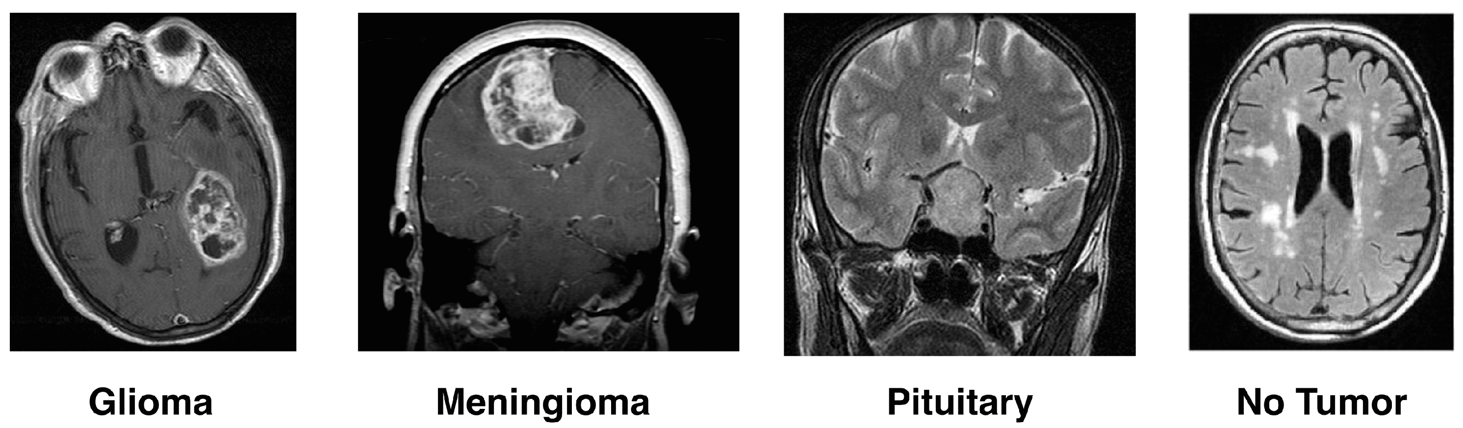
• Gliomas: One type of malignant brain tumor arises from the glial cells that help nourish and protect the brain’s sensory neurons. Glial cells are categorized according to the kind and graded into four grades by the World Health Organization (WHO). Glioblastoma multiforme (GBM) is the most fatal, and Grade IV gliomas have a poor prognosis [14,15].
• Meningioma: These are the membranes that wrap over and around a person’s brain, as well as surrounding their spinal cord, where most benign meningioma tumors usually start. They grow and pressure the brain and other nearby structures, which can cause serious health problems, even if benign. The answer to the problems, usually with surgery well removed, is how recurrence occurs [16].
• Pituitary Tumor: The pituitary gland controls the level of hormones in the body, and these tumors develop there. The vast majority of pituitary tumors (adenomas) are benign but can cause symptoms such as hormonal imbalances. Most often, the treatment involves radiation therapy, surgery, and drugs to control hormone levels [17].
• No-Tumor: Another category of MRI images is harmful, meaning they show tumors. These scans are even used as a benchmark in some research to differentiate between diseased and healthy states. It is necessary to detect and confirm that a tumor is absent for an accurate diagnosis or treatment plan.

1.1. Challenges in Brain Tumor Diagnosis and Classification

The deep learning model can produce effective classification results by carefully preprocessing the images and focusing on their fundamental properties [18]. The intricacy of brain tumors and the intricate structure of the brain can make diagnosis and classification extremely challenging. Magnetic resonance imaging (MRI) is the preferred imaging modality due to its high sensitivity and ability to produce detailed pictures of soft tissues [19]. The labor-intensive and human error-prone manual MRI scan analysis process may lead to inaccurate diagnosis and treatment planning. This indicates the importance of automated and proper diagnostic processes that consistently enable doctors to produce reliable results [16].

1.2. Use of Deep Learning in Classification of Brain Tumors

In the last recent years, great advancements in deep learning have been made, and these may alleviate these problems by automating the identification of brain tumors using the MRI image dataset. Convolutional neural networks (CNNs), such as VGG-16, VGG-19, EfficientNet, MobileNetV2, and others, have demonstrated excellent performance in picture categorization tasks [20,21]. These models can make the difference between the types of brain tumors by identifying and classifying complex patterns and characteristics using previous datasets. Medical imaging deep learning applications can significantly reduce diagnosis time and effort while maximizing accuracy and consistency [22,23].

1.3. Importance of Preparing for Medical Image Analysis

Deep learning models require the preprocessing of MRI images. Grayscale conversion, median and Gaussian blurring noise reduction, video enhancement (Clahe), etc., are the processes that contribute to improving image quality; as a result, relevant features are more prominent [18]. This preprocessing helped the model not only learn to recognize tumors better but also minimize variability. In-depth pre-processing of images allows more focus to be given to these essential features by a deep learning model and leads it to produce efficient classification results [24,25].

After conducting a broad survey in this area, the authors concluded that previous research in this domain has generally struggled to attain high classification accuracy, primarily due to the limited investigation of fine-tuning strategies applied to pre-trained models. To bridge this gap, the present study offers several key contributions:

• Implementation of Fine-Tuning Techniques: Fine-tuning was applied to pre-trained deep learning models, which were then adapted specifically for the target dataset. This approach produced substantial improvements in classification accuracy compared to traditional training or mere feature extraction.
• Comprehensive Experimental Evaluation: A systematic comparison of various fine-tuning strategies and baseline methods was conducted across multiple datasets, providing valuable benchmarks and insights into effective transfer learning practices.
• Practical Guidelines: Clear and actionable recommendations for employing fine-tuning in similar real-world applications are provided, including key optimization strategies and potential pitfalls.

These advancements establish a new standard for effective classification in the domain by overcoming the limitations observed in previous studies and demonstrating the critical impact of fine-tuning on model. he structure of this paper is as follows: Section 2 reviews the current state-of-the-art research relevant to the study. Section 3 details the proposed methodology, outlining the procedures followed throughout the research process. Section 4 presents and discusses the experimental results. Finally, Section 5 concludes the paper by summarizing the key findings, addressing the study’s limitations, and proposing directions for future research.

2. Literature Review

Recent studies have also shown many new and modern methods for classifying brain tumors. For instance, Sleem and Metwaly (2023) demonstrated the use of tailored and fine-tuned deep learning architectures for sensitive academic performance evaluation, offering insights into how domain-specific customization improves classification accuracy. Kumar, P.R., Bonthu, K., Meghana, B., Vani, K.S., Chakrabarti, P., 2023 [25] created an innovative artificial intelligence-based diagnostic strategy for precise identification of diffuse gliomas, applying deep learning models. According to Wadhwa et al. (2019) [26], Machine Learning and Deep Learning models can be used in the identification of brain cancers within MRI scans [27]. While MobileNetV2 remains a highly efficient architecture for lightweight applications, alternative architectures such as EfficientNet and ShuffleNet have also demonstrated promising performance in medical image classification tasks. EfficientNet employs a compound scaling formula to balance depth, width, and resolution, reducing computational costs while maintaining accuracy [28]. Similarly, ShuffleNet optimizes for resource-constrained environments through pointwise group convolutions and channel shuffling techniques [29]. Although this study focuses on MobileNetV2 due to its balance of efficiency and accuracy, exploring other lightweight architectures in future research could further improve tumor classification performance in MRI data. Heang-Ping et al. (2020) presented the real-world benefit of deep learning methods in medical image analysis, highlighting challenges and applications in this domain [22].

On the other hand, Ghadi and Salman (2022) presented a comprehensive review of deep learning-based segmentation and classification techniques for brain tumor MRI. They highlighted the application of these automated procedures in clinical settings [30]. Patil and Kirange (2023) [31] presented the ensemble mechanism of Deep Learning Models for Brain Tumor Detection. In their study, they employed a combination of Shallow Convolutional Neural Networks (SCNN) and the VGG16 network. They created a model that achieved a high classification accuracy of 97.77% in brain tumor segmentation and established robustness instead of overfitting in imbalanced datasets [32]. Ghadi and Salman (2022) also introduced deep convolutional neural networks in MRI images for Classifying Brain Tumors [30]. As suggested in the research 2023 study [31], with the help of deep learning to enhance diagnostic accuracy, they have used.

According to Younis et al. (2022) [33], an innovative method of analyzing brain tumors was described. This method utilized deep learning. The VGG-16 model was especially utilized by the researchers for segmentation and classification. Their research has shown considerable advancements in the accuracy of tumor identification, with the VGG-16 model obtaining an astonishing 98.5% accuracy rate. This demonstrates the model’s potential for accurate and quick diagnosis of brain tumors. The present issues and forthcoming technologies in brain MRI segmentation were investigated by these researchers [33]. Deep learning and the most recent advancements in this area have also been subjected to their scrutiny. Jiang et al. proposed a two-stage cascade U-Net (2020) to acquire great performance outcomes for the segmentation challenge of brain tumor [34].

In their study published in 2020, Aboelenein and colleagues introduced a unique method for brain tumor automatic segmentation that made use of a “Hybrid Two-Track U-Net” (HTTU-Net) architecture [35]. By utilizing the defined two U-Net paths with different layer depths and kernel sizes, this technique combines the outputs of both pathways to achieve more correct segmentation. The method uses focused loss and generalized Dice loss to address the class imbalance. It has shown encouraging results on the BraTS’2018 dataset, which achieved mean Dice scores of 0.865, 0.808, and 0.745 for the total tumor, core, and enhancing areas, respectively [35].

Significant progress was made in the categorization of brain tumors with the use of deep learning beginning in the year 2022. An ensemble of Deep Feature and Machine Learning Classifiers for MRI-Based Brain Tumor by J. Kang, et al. (2024), and MRI-based deep learning models for brain tumor classification are among the contributions [36]. Sleem and Metwaly (2023) studied a deep learning-based model for evaluating academic performance using student behavior patterns, which provides a fine-tuned deep learning architecture applied to sensitive classification problems is presented this research work [37]. Tolba and Fathy (2023) in Chaotic metaheuristic optimization for improving text classification performance offer insights into model optimization relevant to CNN-based medical classification is studied in the work [38]. These researchs [37,38] provides a good overview of the implemenation of machine learning in real life.

Various contributions include various models. Both the construction of hybrid models for performance analysis and the enhancement of classification accuracy based on transfer learning and deep learning approaches are two additional key areas of study [39].

Using Magnetic Resonance Imaging (MRI), deep convolutional neural networks (CNNs) have shown substantial potential in the classification of brain tumours, according to Gómez-Guzmán et al. (2023) [40,41]. A total of seven different CNN models were assessed in their research, including the pre-trained models such as InceptionV3, which created an accuracy of 97.12% (Gómez-Guzmán et al., 2023) [41]. CNNs can improve diagnostic accuracy and help doctors in the early diagnosis of brain tumours, as shown by this scenario. In the field of medical diagnostics, the use of deep learning methods in the categorisation of brain tumours is a significant advancement. Robust neural network topologies, such as MobileNetV2, that may be used in conjunction with sophisticated preprocessing techniques to attain a high level of accuracy at the time of tumour classification [41,42]. At the end of the day, this helps treatment planning as well as communication with patients. The authors of this research have shown the way to efficiently train lightweight CNNs for medical picture categorisation tasks without sacrificing performance, using specialised training schemes [42].

To classify brain tumour, Akter et al. (2024) presented a deep convolutional neural network (CNN) architecture that was combined with a U-Net-based segmentation model [43]. This combination resulted in exceptional accuracy. Following extensive testing on six benchmarked datasets, the classification model obtained an accuracy of 98.7% on a merged dataset and 98.8% using the segmentation technique. This was accomplished by combining the datasets [43].

A similar approach was presented by Rasheed et al. (2023) [44]. This study has proposed a great technique using Gaussian-blur-based sharpening and Adaptive Histogram Equalisation (CLAHE). A remarkable classification accuracy of 97.84% has been achieved by this study, with precision, recall, and F1-score values that were all higher than 97%. Comparing the results of this research with those of pre-trained models such as VGG16, ResNet50, and MobileNetV2 demonstrates how successful the improvement strategies used by these models are in improving classification results. This approach is notable not only for its high accuracy but also for its ability to generalize effectively across a variety of brain tumors, such as glioma, meningioma, and pituitary tumors, all of which are examples of brain tumors [44].

A detailed assessment of several deep convolutional neural network (CNN) models was carried out by Gómez-Guzmán et al. (2023) to identify brain tumours with the use of magnetic resonance imaging (MRI) [41]. They investigated seven CNN models, including a generic CNN as well as six pre-trained models, to evaluate how good they were in classifying brain tumours. In this study, a dataset of four categories of MRI images (3 types of brain tumors and healthy brains) was used to classify the 7023 MRI images. Several preprocessing approaches were applied to the MRI images by the authors, and then they compared the performance of several CNN models, including ResNet50, InceptionV3, InceptionResNetV2, Xception, MobileNetV2, and EfficientNet with one another. The InceptionV3 model was the most successful Deep Learning model in this study. This study achieved an accuracy rate of 97.12% on average [41].

The results of this research emphasise the potential of the InceptionV3 model in the identification and classification of brain tumour MRI images. This could help physicians identify and initiate large-scale treatment of brain malignancies. Through this method, they focused on the significance of sophisticated deep learning techniques in the field of medical imaging. This approach provides a solid framework for enhancing diagnostic accuracy and assisting in the selection of therapeutic decisions.

3. Methodology

The methodology section explains the data (dataset, preprocessing), model findings, and evaluation metrics used in this study. Every step is crucial to achieving high accuracy in brain tumor classification.

3.1. Dataset Description

In this study, there has been used a publicly available MRI dataset, Msoud [45] from Kaggle has been used. This dataset consists of the three publicly accessible datasets, including Figshare [46], SARTAJ [45], and BR35H [47] images for four classes: glioma, meningioma, pituitary tumor, and no-tumor, is shown in Figure 1. The data is segregated into two main sub-folders (Training and Testing). The dataset was pre-partitioned into training and testing subsets, comprising 5712 training and 1311 testing images, distributed proportionately across the four classes. The original dataset authors provided this pre-partitioning to ensure fairness and prevent data leakage. The distribution of training and testing sets was retrospectively analyzed to confirm balanced representation, as shown in 

Table 1. Percentile Distribution of Train data and Test data.

Class	Train Images	Train Percent	Test Images	Test Percent	Test Ratio
Glioma	1321	23.1	300	22.9	22.7
Meningioma	1339	23.4	306	23.3	22.9
No tumor	1595	27.9	405	30.9	25.4
Pituitary	1457	25.5	300	22.9	20.6
Total	5712	100	1311	100	22.95 Avg

.

By adhering to the pre-defined training and testing splits, this study ensures consistency and comparability with previous research that employs the same dataset. Analyzing the dataset’s class distribution (Table 1), it is evident that there is a significant class imbalance. The “No Tumor” class, with only 523 images, is notably smaller compared to the other classes, such as Glioma and Pituitary (2000 images). This imbalance may lead to biased model performance and pose challenges in achieving uniform sensitivity across all classes.

3.2. Preprocessing

This research developed a new preprocessing was applied to ensure the MRI images were optimized for effective learning and classification by the MobileNetV2 model. Each step in the preprocessing pipeline was carefully designed to address challenges in medical imaging, such as noise, varying intensities, and anatomical variability. These steps improve the interpretability of MRI images and enhance the ability of the deep learning model to extract meaningful features when detecting and classifying brain tumors. The mechanism of attributes divides the function into several parts, as shown in Figure 2.

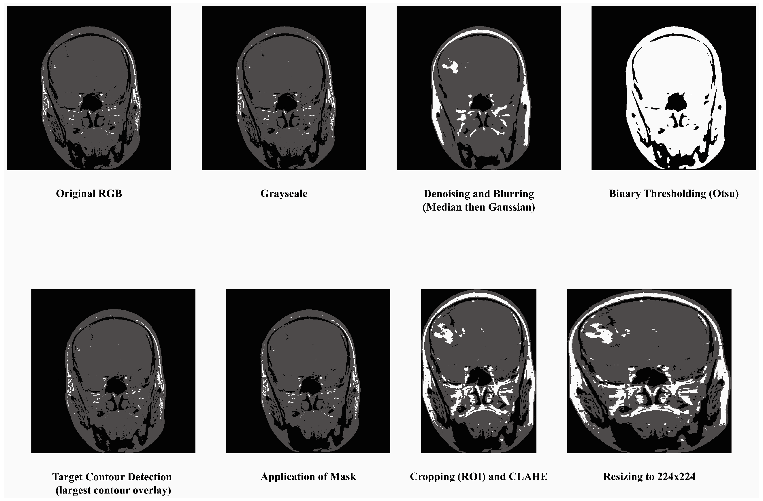
• Convert to Grayscale: Most MRI datasets are in grayscale or captured using only intensity-based information, while some datasets may also include unnecessary color channels (from RGB formats). Converting them to grayscale ensures uniformity in data representation and reduces computation by eliminating redundant information. The process has been done by grayscale using OpenCV’s cv2.cvtColor function. This step also helps focus the model on texture and contrast, which are critical for identifying tumor regions in medical imaging.
• Denoising and Blurring: MRI images often contain artifacts or noise due to acquisition methods, which can obscure key tumor features. Median filtering reduces random noise, preserving the edges and fine details critical for classification without distorting important structures like tumor contours. Blurring is applied to smooth the image and reduce high-frequency variations unrelated to tumors. It helps in suppressing minor unrelated details (e.g., scanner irregularities) and enhances the model’s ability to focus on regional features of tumors rather than noise.
• Binary Thresholding: Binary thresholding creates a clear separation of foreground (possible tumor areas) and background, which aids in isolating the tumor region. By emphasizing areas of interest based on intensity standards, this step generates a mask for tumors, facilitating structured feature extraction and segmentation. The method was applied using a fixed threshold value of 127. This process created a binary mask for tumor region selection. For normalization, pixel intensity ranges were scaled between 0 and 1 prior to thresholding.
• Target Contour Detection: After applying the binary mask, it is essential to extract the tumor region accurately. The contour detection algorithm identifies and segments the largest connected region (potential tumor) and removes non-relevant regions such as background noise or anatomical elements outside the tumor that has been done using findContours function in Python’s OpenCV library. That finds the largest contour by area greater than 500 pixels was selected as the tumor region. This ensures the model focuses on the most relevant part of the image.
• Application of Mask: The binary mask is directly applied to filter out regions irrelevant to the tumor. It allows the model to operate only on imaged regions that likely hold tumor information, improving classification accuracy and computational efficiency.
• Cropping, CLAHE: After isolating the tumor, extracting the region of interest (ROI) eliminates unnecessary background, allowing the model to focus entirely on meaningful features while standardizing input dimensions. This technique enhances the contrast of the tumor region by redistributing brightness in the image, helping highlight subtle details. CLAHE with clip limit = 2.0, grid size = (8 × 8), that reduces the inter-image variability caused by differences in MRI scanner settings, patient anatomy, or lighting conditions, which are particularly important for tumor region detection [48].
• Resizing: To ensure compatibility with the MobileNetV2 architecture, all images are resized to a fixed dimension of 224 × 224 pixels. This step provides uniformity in input size, reduces computational demands, and ensures that the model processes images efficiently without distortion.

The Original MRI image and preprocessed final image of the Pituitary, Meningioma, Glioma, and No Tumor are shown in Figure 3a–d.

The preprocessing outcomes were visually validated by analyzing the images before and after applying techniques like grayscale conversion, CLAHE, Gaussian noise reduction filter with a 5 × 5 kernel, and cropping of the tumor region. The improvements in contrast and noise reduction were observed to bring out clear tumor textures, which are essential for subsequent classification. The incorporation of preprocessing techniques enhances the model’s ability to extract key tumor features by improving image contrast and reducing noise, respectively. As a result, the model avoids overfitting to irrelevant details and focuses on important tumor-specific patterns, contributing to improved classification accuracy.

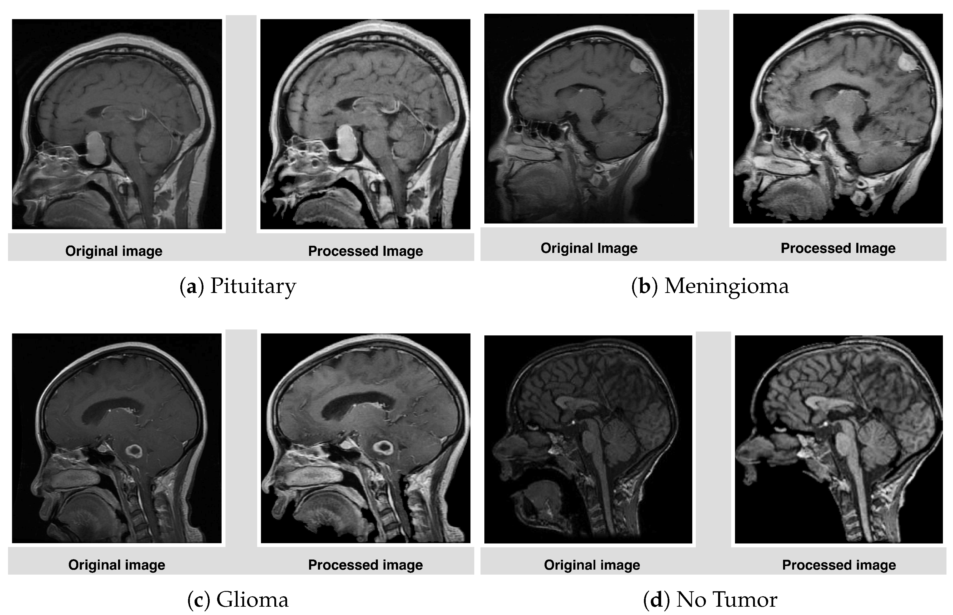
3.3. Anatomical and Imaging Considerations in Dataset Construction

The MRI images included in this study reflect not only tumor pathology but also variability arising from anatomical and imaging factors. Each tumor type displays unique anatomical patterns: gliomas often infiltrate neighboring tissues, resulting in poorly defined boundaries on MRI; meningiomas, being extra-axial, cause local distortion of adjacent structures; and pituitary tumors are located centrally, sometimes compressing the optic chiasm or invading the cavernous sinus, affecting local anatomy. Imaging factors also impact dataset consistency—differences in scanner hardware, magnetic field strength, patient movement, and acquisition protocols can introduce noise, variability in contrast, or subtle artifacts. The ‘no tumor’ images may also vary in anatomical presentation due to age, brain size, or incidental findings. These anatomical and imaging variances may complicate tumor localization and classification, and justify the rigorous preprocessing and normalization procedures described in Section 3.2. By integrating these diverse images, the dataset provides a realistic clinical spectrum, but also presents additional challenges for automated methods, highlighting the need for robust preprocessing and model selection.

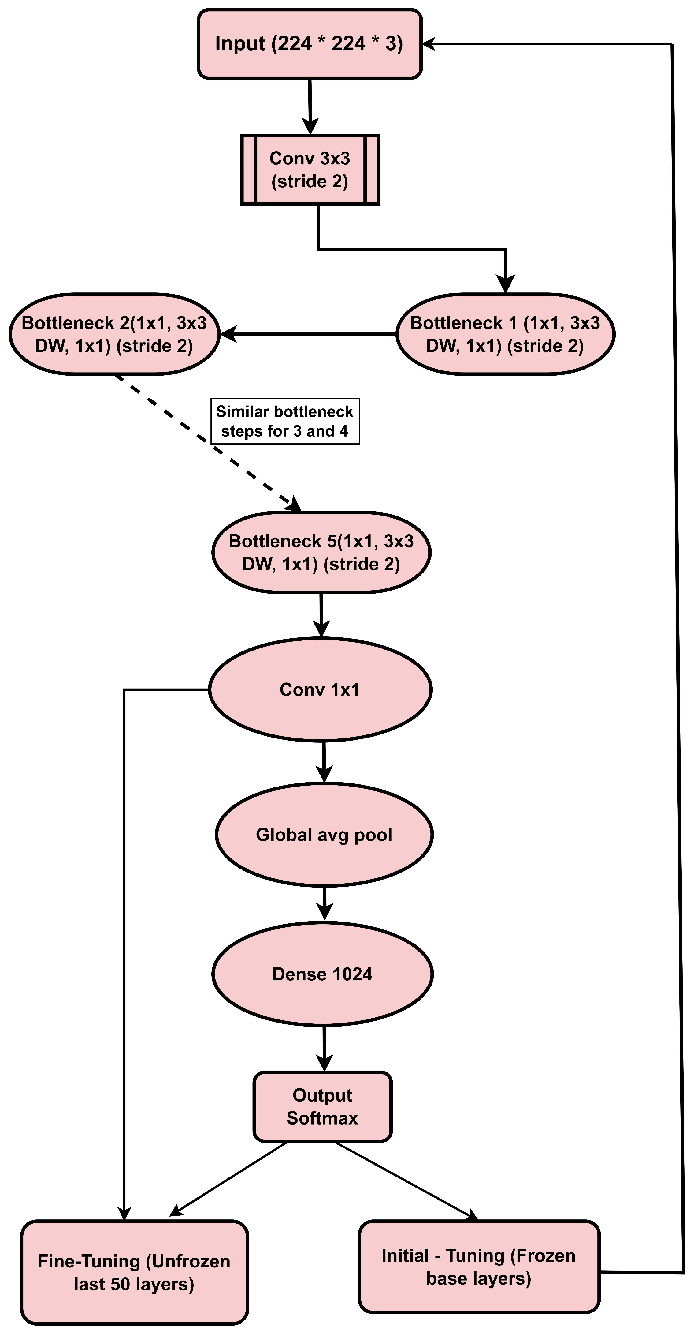
3.4. MobileNetV2 Architecture

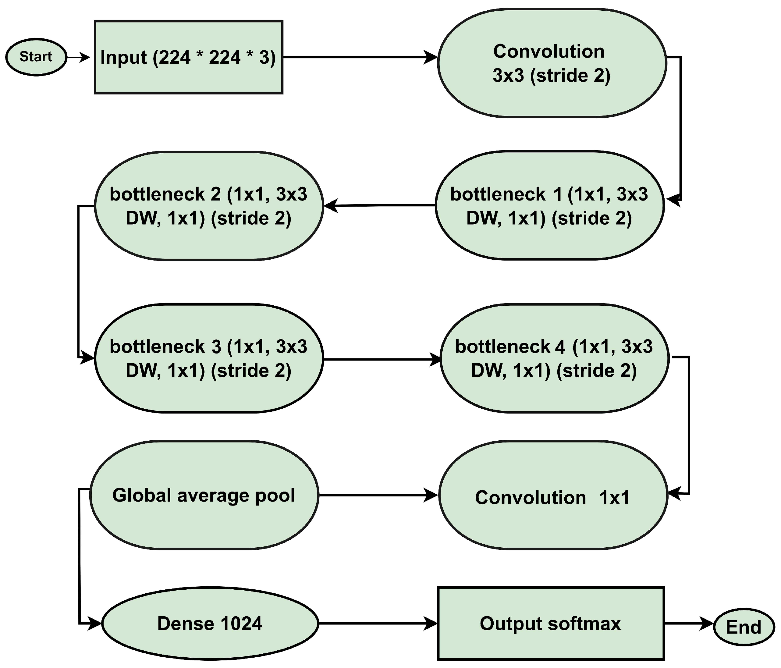
MobileNetV2 is a Machine Learning model class for Mobile Networks that makes extensive use of depth-wise separable convolutions to build very small deep networks. It uses depthwise separable convolutions to decrease parameter count and consequently has an order of magnitude less cost of computation. This research utilized an architecture (MobileNetV2) pre-trained on ImageNet, which was then fine-tuned using the dataset for brain tumor classification. MobileNetV2 was chosen due to its lightweight architecture, which allows for reduced computational cost while delivering high accuracy. This is particularly advantageous for medical imaging tasks like brain tumor classification, where intricate patterns in MRI images need to be captured effectively. The use of depthwise separable convolutions ensures efficient feature extraction with significantly fewer parameters compared to models like VGG16 or ResNet50. Furthermore, the pre-trained ImageNet weights help accelerate convergence while allowing the architecture to adapt effectively during fine-tuning. In comparison to heavier models like InceptionV3 or EfficientNet, MobileNetV2 achieves an optimal balance between accuracy and computational efficiency, making it ideal for resource-constrained environments such as real-time diagnostic imaging. The basic layers in the MobileNetV2 architecture are shown in Figure 4, are explained in detail in the following subsequent sections.

3.4.1. Input Layer

The input layer marks the start of the neural network. It takes as input images that have been processed in previous data preprocessing steps. Following the requirements of the neural network, each image is resized to standardized dimensions of 224 × 224 pixels. Moreover, the input layer accepts images with 3 channels corresponding to the RGB color model, which guarantees compatibility with color image datasets. This layer ensures that the model receives inputs that are formatted consistently to enable effortless feature learning from visual data, which is pivotal for model training and evaluation.

3.4.2. Convolutional Layer (Conv 3 × 3, Stride 2)

The previous layer is also responsible for passing down images to the subsequent layers. The image is extracted together with its bounding box as a component of the initial data collection stage. Following this, the convolutional layer carries out convolution using a 3 × 3 kernel (filter) on the image obtained from the previous layer. The stride of 2 allows the convolution step to perform a reduction of the image spatial dimensions. The width and height are reduced by half over consecutive operations. This reduction not only saves computational power but also significantly enhances powerful localized features through hierarchical feature extraction.

$$(I\ast K)(i\ast j)=\sum _m\sum _{n}I(i+m,j+n)·K(m,n)$$

(1)

where I represents the input image matrix, K represents the convolution kernel (filter) matrix, i, j are the coordinates in the output feature map, m, n are the indices for iterating over the kernel elements.

3.4.3. Depthwise Separable Convolutions

The depthwise separable convolution layer is an operation in lightweight neural networks such as MobileNetV2 that aims to extract features with minimal computational resources. This layer can be divided into two sub-layers: Depthwise Convolution and Pointwise Convolution.

The Depthwise Convolution filters the input using one convolutional filter per channel, which reduces the complexity of calculations. After the depthwise convolution, pointwise convolution or adding 1-by-1 convolutions with channels of 3-by-3 is done, which enhances cross-channel communication while maintaining spatial resolution. These result in more efficient feature extraction with less computational cost compared to traditional convolution methods.

3.4.4. Bottleneck Layers

The bottleneck layers employ a set of 1 × 1 convolutions, depthwise convolution, and expand the dimension using another set of 1 × 1 kernels. These layers are designed to capture the spatial features at various filter data granules and effectively balance the network structure to optimize the computational load and feature extraction.

3.4.5. ReLU6 Activation

The ReLU6 activation, which restricts its output to 6, especially for mobile devices, adds critical non-linearity to the network and enhances numerical stability. This can be expressed as follows: f(x) = max(0,x). ReLU variants are widely known for their stability. However, the straightforward version is suboptimal for mobile and embedded systems, which makes this variant preferable.

3.4.6. Batch Normalization

Batch normalization (Batch Norm) is a technique that recovers the speed of the previous layers through the normalization of the output of the previous layers and improves the convergence of the model. It can be represented mathematically as:

$$x^k={\displaystyle \frac{x^k-{\mu }_b}{\sqrt{{{\sigma }_B}^2+ϵ}}}$$

(2)

where $x^k$ represents the normalized output, ${\mu }_b$ is the mini-batch mean, ${\sigma }_b^2$ is the mini-batch variance, and $ϵ$ is a small constant for numerical stability (typically ${10}^{-5}$).

3.4.7. Global Average Pooling (GAP)

Global Average Pooling (GAP) is a technique used for dimensionality reduction. The procedure works as follows: it takes the average of the feature map over all of its spatial dimensions instead of forming many dense layers with a big number of parameters to find the right low-dimensional configurations for projecting spatial features. In other words, GAP directly collapses the width and height of the feature maps to one, for each channel, instead of feeding the network with fully connected layers with a high number of weights. Thus, consequently, the layer’s output is shaped as a vector with a length equal to the number of feature map channels. The GAP can be presented as

$${\mathbf{y}}_{\mathbf{c}}={\displaystyle \frac{1}{H\ast W}}\sum _{i=1}^H\sum _{j=1}^W{x}_{ijc}$$

(3)

where $y_c$ represents the output for channel c, W is the width of the feature map, H is the height of the feature map, $x_{ijc}$ represents the pixel value at position $(i,j)$ in channel c, and ${\sum }_{i=1}^H{\sum }_{j=1}^W$ indicates summation over both i and j dimensions from 1 to H and 1 to W respectively.

3.4.8. Fully Connected Layer (Dense Layer)

The fully connected (dense) layer acts as the last stage where the features that are extracted by the previous convolutional and pooling layers are aggregated to ensure that the necessary predictions are made. The layer in the given model consists of 1024 units, which makes it possible for it to be able to acquire complex and high-level patterns necessary for accurate classification. Every unit from the previous layer is connected to the one in this layer, which is the leading cause of the formation of the non-linear mappings and relations between the features. Incorporating the ReLU function in the dense layer prevents overfitting and accordingly improves model performance by allowing the introduction of non-linearity into the network. ReLU function guarantees that only the positive values are carried forward from the features, thus making the irrelevant or negative ones be discarded effectively if any.

3.4.9. Output Layer (Softmax)

The end layer shifts the entire set of descriptive features to the predicted probability of each class. The Softmax activation function is applied so that the predicted values are interpretable as probabilities and sum to 1. To be specific, the Softmax function sends out a vector of the same length as the number of classes existing, with each element signifying the model’s prediction that the input belongs to that class. The softmax function is the one that makes it possible to single out the right class by the highest probability. It so happens that it boosts the true class and drops the others, thus influencing the multi-class classification. This component of the network is the final deciding part, which provides outputs for the evaluation or the deployment. It can be defined mathematically as

$$\sigma {\left(z\right)}_i={\displaystyle \frac{e^{zi}}{{\sum }_{K=1}^K{e}^{zk}}}$$

(4)

where $\sigma {\left(z\right)}_i$ represents the softmax output probability for each class i, $z_i$ is the input for a class i, K represents the total number of classes, e is the exponential function, and ${\sum }_{k=1}^K$ indicates summation over all classes from 1 to K. The function normalizes the exponential values such that all outputs sum to 1, providing a probability distribution across all classes.

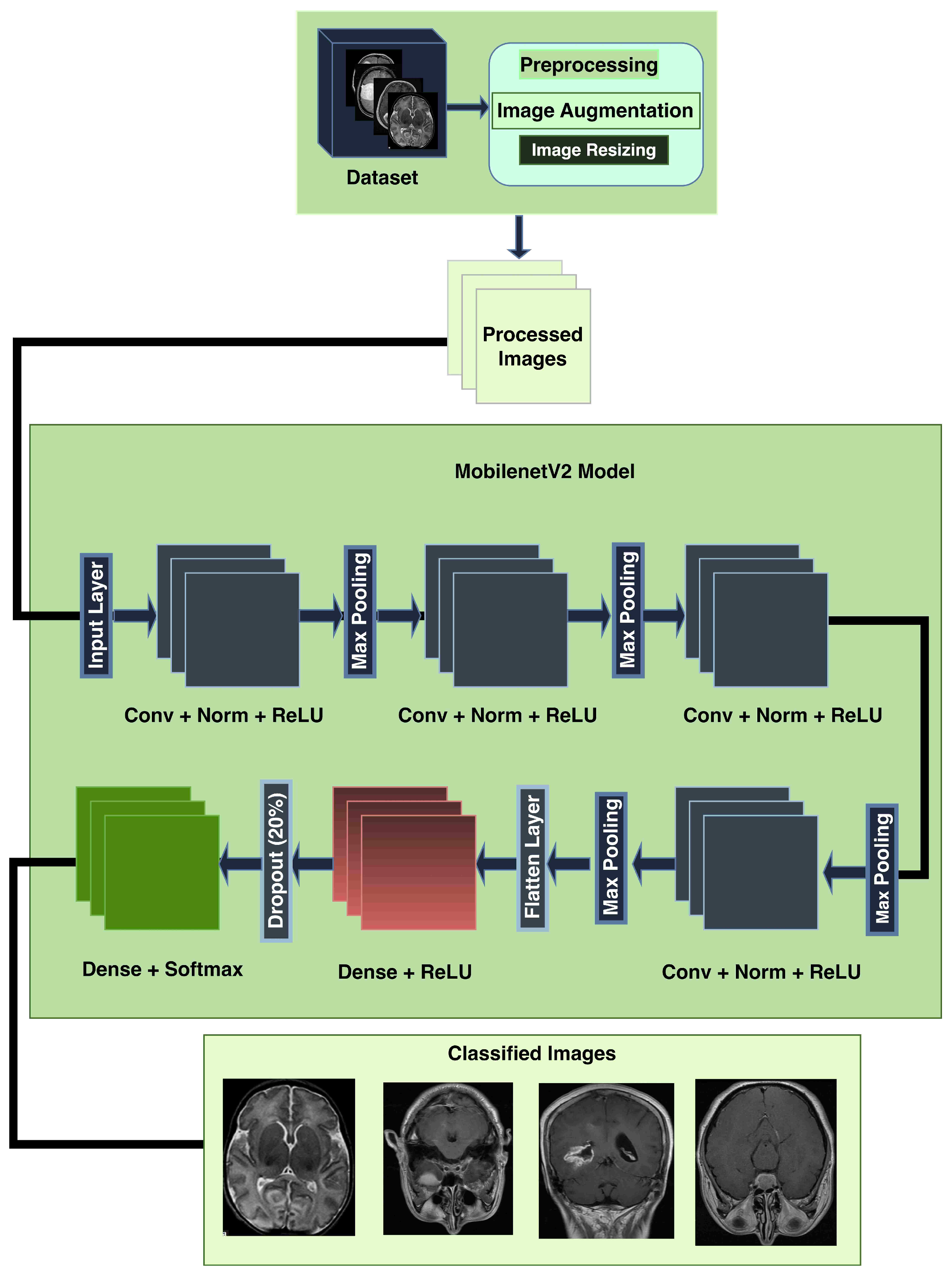
3.5. Operational Model

The overall architecture of the operational model for the MobileNetV2 that is utilized for the classification of brain tumors based on MRI images is presented in Figure 5. The procedure can be divided into three primary stages: data pre-processing, MobileNetV2 architecture, and final classification identification.

During the first stage of the process, the raw MRI images are subjected to preprocessing, which includes performing the following steps:

• Image Augmentation: Data augmentation was applied in the training dataset to improve the generalization of the model by expanding the dataset artificially. The applied techniques included horizontal flips, vertical flips, random rotations within the range of $\pm {90}^{\circ }$ to simulate variations in imaging position, and slight translations (up to $\pm 10\%$ of the image dimensions). Care was taken to ensure anatomically relevant image preservation by avoiding excessive rotations or distortions that could affect key characteristics of the brain tumor regions. These transformations were implemented in TensorFlow’s ImageDataGenerator, which automatically manages consistent application across the dataset to prevent misaligned augmentation effects. Data augmentation is very effective in boosting performance for minority classes. Despite the data imbalances, the model maintains robust performance across all classes.
• Image Resizing: All of the images are resized so that they conform to the specifications that MobileNetV2 requires for input (for example, 224 by 224 pixels).
• Normalisation: Images are normalised to ensure that the intensities of each pixel are consistent for effective learning. As input, the images that have been preprocessed are introduced into the MobileNetV2 model.

In the second stage of the process, the MobileNetV2 architecture is made up of several convolutional layers that are interspersed with batch normalisation, ReLU6 activations, and max pooling layers. One of the most well-known characteristics of the MobileNetV2 model is its effectiveness in feature extraction through the utilisation of depthwise separable convolutions:

• Feature Extraction: Extracting features at multiple levels is what convolutional layers are all about.
• Batch Normalization: Batch Normalization is a process that normalizes the outputs of layers to guarantee stable and effective training.
• ReLU6 activation: The ReLU6 activation increases the amount of non-linearity while preserving the numerical predictability.
• Max Pooling: Max Pooling Layers can reduce the spatial dimensions while still preserving the essential characteristics.
• Dense layers: To pass on the features that were extracted from these layers to the dense layers, they are first flattened.

In the third stage of the process, the flattened features are processed by the dense layers, which then use the softmax activation function to predict the type of tumour class using probabilistic outputs:

• Extraction of high-level representations from the feature space is accomplished by the Dense Layer with ReLU Activation system.
• Using a random deactivation of neurons, the Dropout Layer prevents overfitting from occurring.
• The output of the Dense Layer with Softmax Activation is a probability distribution that accounts for all of the tumour classes.

Finally, the images classified are placed into one of the following four categories of tumors: glioma, meningioma, pituitary tumor, or no tumor.

3.6. Proposed Model

The architecture for the custom prejudicing model is similar, except that it is only trained on new preprocessed images produced by our custom preprocessing function. In this way, the shape of the model better represents only the upgraded and limited tumor regions, possibly allowing the model to achieve higher classification accuracies. Our proposed overall architecture is presented in Figure 6.

In Figure 6, there are two main steps to the training process: (1) initial parameter training with freezing base layers and recycling through batch normalization scaling factors (the model is claimed to be deterministic after that), (2) fine-tuning by fully unfreezing the last n = 50 conv4 torch virsion models accompanied by another tweak in the learning policy schedule for distributed spec care settlement.

The detailed as well as technical architecture of the proposed model is illustrated in Figure 7. This modular system is divided into three key components: frozen layers, fine-tuned bottleneck layers, and the custom fully tuned classification head. These components work together to efficiently extract features, adapt the network to domain-specific MRI data, and produce precise tumor classifications. A critical step in this architecture is the fine-tuning process, which strategically adjusts portions of the network for optimal performance. The details explanation is discussed in the following subsequent sections.

3.6.1. Initial Training (Feature Extraction Stage)

In this stage, the base layers of the pre-trained MobileNetV2 model (trained on ImageNet) were frozen to retain general feature representations. Only the custom dense head layers were trained during this step to adapt the general features to the task-specific dataset. Empirical testing showed that freezing base layers while training only the dense layers achieved stable convergence. The batch normalization scaling factors of the frozen layers were fine-tuned to ensure compatibility with the task-specific data, ensuring robust performance.

• Training Base Layers: Initially, the base layers of the pre-trained model (MobileNetV2) are frozen so that they retain features learned from the large ImageNet dataset. Train only the new dense layers.
• Data Augmentation: It uses techniques like horizontal flip, longitudinal flip, and random rotations to perform Data augmentation on images used in training the model by adding variations.
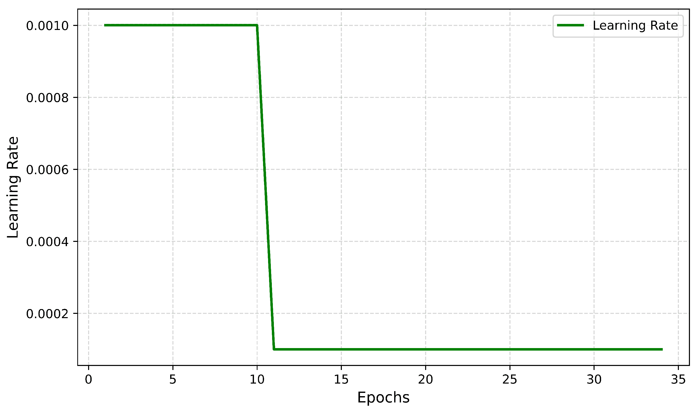
• Training: The model trains a fixed number of epochs with the optimizer set as Adam, learning rate = 0.001.

To determine the optimal configuration, a lightweight hyperparameter search was conducted with adjustments to the learning rate (0.01, 0.001, 0.0001), number of unfrozen layers (25, 50, 75), and optimizers (Adam, SGD). The final configuration of 50 unfrozen layers, 0.0001 learning rate, and the Adam optimizer provided the best performance metrics, balancing validation accuracy (99.16%) and computational efficiency.

3.6.2. Fine-Tuning/Learning Weight Adjustment

After the initial training, the last 50 layers of the MobileNetV2 model were unfrozen for fine-tuning. To determine the number of layers to unfreeze (n = 50), lightweight experimentation was conducted with different values, and the best results were observed when fine-tuning the last 50 layers.

• Frozen Based Last 50 Layers: Training from scratch, then unfreezing the last 50 layers of the MobilenetV2 base model for fine-tuning.
• Lower Learning Rate: The learning rate is decreased to 0.0001 to adjust the model more accurately.
• Early Stopping: This research used early stopping to avoid overfitting and maintain stable performance on new data.

Additionally, the learning policy schedule was adjusted, and a grid search was performed to optimize the learning rate (0.01, 0.001, 0.0001), with the best results observed for 0.0001. The Adam optimizer was chosen after empirical comparison with SGD, which showed slightly lower validation accuracy and longer convergence times.

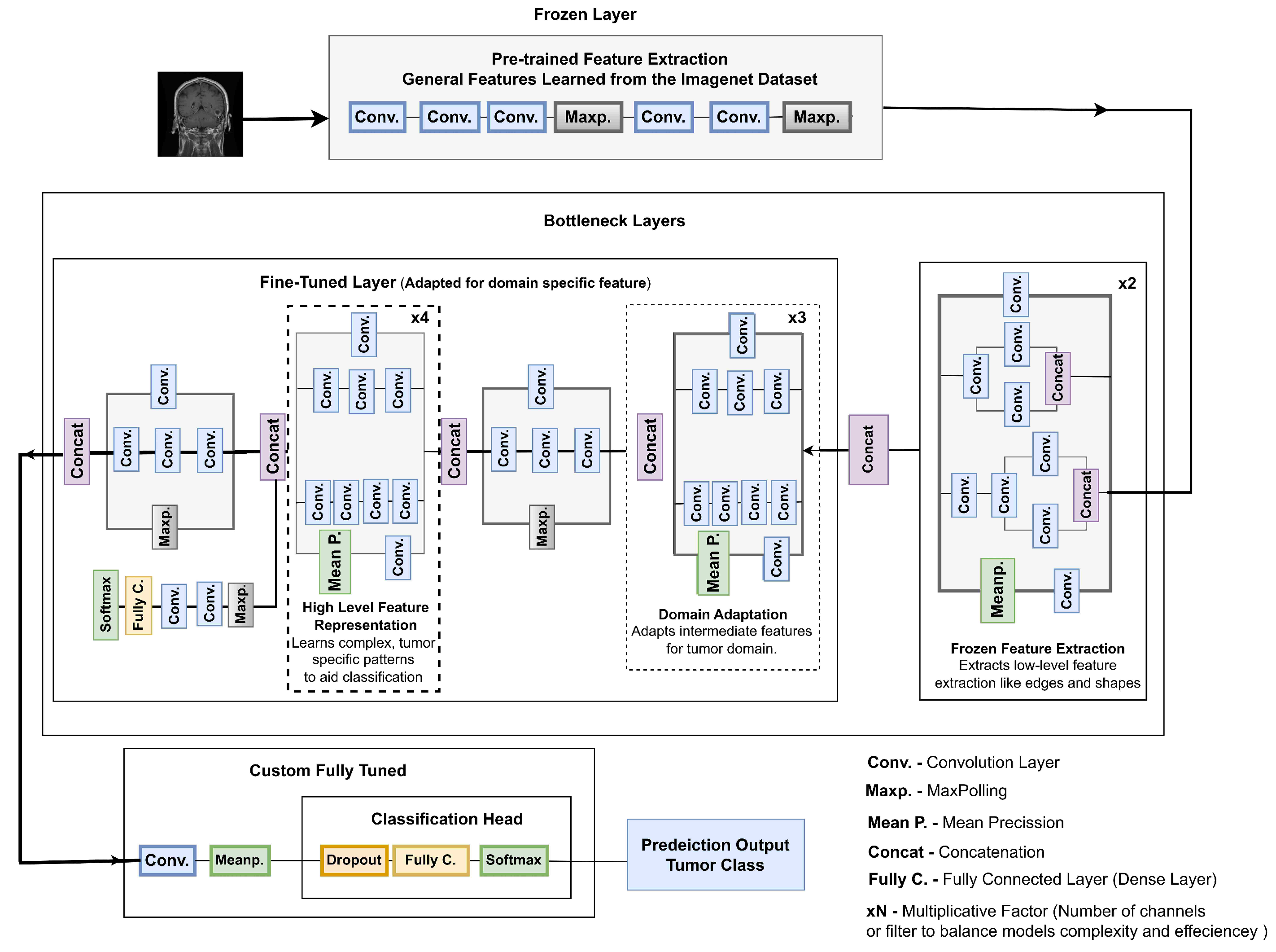
3.6.3. Frozen Layers

The Frozen Layers utilize pre-trained MobileNetV2 weights trained on the ImageNet dataset, which are kept fixed to retain their ability to extract generic low-level features, such as shapes, edges, and textures. These features are integral across most image classification tasks. Since these layers capture universal patterns, they remain unchanged during training and provide a solid foundation for further domain-specific adaptations. The outputs from this stage are forwarded to the bottleneck layers.

3.6.4. Fine-Tuned Bottleneck Layers

The Fine-Tuned Bottleneck Layers are central to the proposed architecture, enabling the model to adapt pre-trained features for brain tumor classification with efficient computational costs. These layers, structured as ×2, ×3, and ×4 bottlenecks, operate independently to extract task-relevant features with parameter counts and FLOPs (Millions) detailed below the

Table 2. Computational Details of Bottleneck Layer.

Bottleneck Layer	Parameter Count	FLOPs (Millions)
×2	0.5	5.0
×3	1.0	10.0
×4	1.9	15.0

. After the initial training, the last 50 layers of the MobileNetV2 model were unfrozen for fine-tuning. Lightweight experimentation was conducted with different values, and the best results were observed when fine-tuning the last 50 layers. This depth allowed the model to adapt domain-specific patterns such as subtle tumor structures, while preserving the general features extracted by the frozen base layers. Selective unfreezing prioritizes higher-level feature representations specific to glioma, meningioma, and other brain tumor types, enhancing the model’s classification performance.

• ×2 Bottleneck: This initial layer utilizes pre-trained ImageNet weights and extracts low-level features such as lines, edges, and textures. By keeping this layer frozen, fundamental knowledge is preserved while avoiding overfitting to noise. As shown in Figure 6, it lays the foundation for domain-specific refinement with a minimal computational cost of 0.5 M parameters and 5.0 M FLOPs.
• ×3 Bottleneck: The intermediate ×3 bottleneck transitions from low-level to medium-level feature extraction, capturing region-level details and textural differences in MRI images. This layer bridges general features with domain-specific attributes for tumor classification. As depicted in Figure 7, it enables the model to focus on relevant sections without disrupting previously learned weights. This stage has a computational cost of 1.0 M parameters and 10.0 M FLOPs.
• ×4 Bottleneck: The ×4 bottleneck focuses on extracting high-level tumor-specific features, crucial for distinguishing between tumor classes such as gliomas, meningiomas, and pituitary tumors. Fine-tuning this layer enhances the model’s ability to identify complex patterns, ensuring accurate segmentation and classification, achieved with 1.9 M parameters and 15.0 M FLOPs.

Both ×3 and ×4 bottlenecks play a critical role in domain adaptation by extracting specific and intricate tumor-related features from MRI scans. Figure 7 illustrates the architecture’s complexity and the interaction of specialized layers, contributing to the final classification output. Freezing early layers preserves general features, while fine-tuning later layers adapts the model to tumor-specific features in MRI images. This combination ensures efficient learning without overfitting, leading to improved tumor identification, particularly in overlapping classes such as meningioma and pituitary tumors.

3.6.5. Depthwise Separable Convolutions

Within all bottleneck layers, the use of depthwise separable convolutions ensures that the model efficiently processes features while minimizing computational costs. This architecture supports a lightweight structure while simultaneously allowing for rich, informative feature extraction necessary for effective classification.

3.6.6. Integration of Fully Tuned Layers

The Custom Fully Tuned Classification Head is fully retrained specifically for the brain tumor dataset. This stage ensures the network can classify tumors with optimal accuracy while integrating the generalized and fine-tuned features from earlier stages. The classification head performs the following tasks:

• Processes the features passed from the fine-tuned bottlenecks through:

  -

  A dropout layer to prevent overfitting, where the dropout rate was set to 20% in the dense layers after the ReLU activation and before the softmax layer during both initial and fine-tuning training phases.

  -

  Fully connected dense layers to aggregate and refine features into class-specific representations.

• Classifies the output into one of four classes: pituitary tumor, glioma, meningioma, and no tumor. It uses the softmax activation function to output probabilities for each class.

3.6.7. Why Fine-Tuning Is Crucial

Figure 7 demonstrates how fine-tuning selectively specializes the model for the brain tumor classification task while maintaining the computational efficiencies of the pre-trained MobileNetV2 architecture. By retraining only the later layers (×3 and ×4 bottlenecks), the model effectively learns tumor-specific patterns without compromising general feature extraction. This process highlights the importance of balancing transfer learning (reusing frozen features) with task-specific adaptations.

The integration of the fully tuned classification head completes the architecture, combining domain-specific feature extraction with class prediction, leading to a robust and efficient model for brain tumor classification.

3.7. Evaluation Metrics

In this study, the performance of the proposed brain tumor classification model is analyzed using multiple evaluation metrics. These metrics are defined and explained further in this document. They not only determine how well the model performs but also provide insights into how balanced it is across all types of tumors, while ensuring consistent results even in the presence of class imbalance.

Moreover, achieving high classification accuracy is crucial for the well-being of patients and their treatment management. For these reasons, a combination of metrics, such as accuracy, precision, recall, F1-score, Cohen’s Kappa Score, and the Matthews Correlation Coefficient (MCC)—is used to evaluate the effectiveness of the brain tumor classification model.

For each metric, its definition, significance, and relevance to this study are provided. In the subsequent sections, these measures are discussed in relation to the classification problem, ensuring not only the effectiveness of the model but also its reliability and balance across all tumor types, regardless of the presence of class imbalance.

3.7.1. Accuracy

The accuracy metric quantifies the number of accurate predictions relative to the total number of predictions made. The accuracy can be defined as:

$$\mathrm{Accuracy}={\displaystyle \frac{\mathrm{TP}+\mathrm{TN}}{\mathrm{TP}+\mathrm{TN}+\mathrm{FP}+\mathrm{FN}}}$$

(5)

where TP is the number of correctly predicted positive cases and TN represents the number of correctly predicted negative cases. FP presents the number of negative cases incorrectly classified as positive, and FN presents the number of positive cases incorrectly classified as negative [49,50].

3.7.2. Precision

To avoid false positives, precision measures a model’s positive predictive accuracy by assessing the fraction of true positive samples predicted. It can be expressed mathematically as:

$$\mathrm{Precision}={\displaystyle \frac{\mathrm{TP}}{\mathrm{TP}+\mathrm{FP}}}$$

(6)

For tumor classification, precision is important in reducing false-positive diagnoses. For example, identifying a tumor on an ordinary brain scan can result in superfluous interventions and distress among patients. A model with high precision is more likely to be accurate with predicting a tumor. In the positive class of cases, the precision indicates the reliability of the model in clinical settings.

3.7.3. Recall/Sensitivity

Recall, often known as sensitivity, gauges how well the model accurately classifies positive samples. It can be defined as:

$$\mathrm{Recall}={\displaystyle \frac{\mathrm{TP}}{\mathrm{TP}+\mathrm{FN}}}$$

(7)

In medical imaging, recall is arguably the most important aspect to consider, as failing to identify a tumor (false negatives) may prove fatal to a patient. Having a high recall guarantees that the model captures all true tumor cases, making it very important alongside precision. This analysis pays a lot of attention to recall since its inherent cost–missing a tumor–is far greater, and more severe, than a false positive.

3.7.4. F1-Score

The F1-score calculates the weighted average of precision and recall through their harmonic mean, combining both values in a singular score [50]. This can be expressed as follows:

$$F1=2\ast {\displaystyle \frac{\mathrm{Precision}\ast \mathrm{Recall}}{\mathrm{Precision}+\mathrm{Recall}}}$$

(8)

When classifying problems such as brain tumor detection, where datasets often have class imbalance, the F1 score provides a more accurate measure of value. This number is most useful in cases when there is a trade-off between precision and recall, as it gives them equal weight. A high score on this metric indicates that the model correctly identifies true positives, such as tumors, while also avoiding a large number of false positives.

3.7.5. Specificity

Specificity is a critical evaluation metric in medical diagnostic systems. It measures the proportion of correctly identified negative cases (true negatives) out of all actual negative cases. Specificity is formally defined as:

$$\mathrm{Specificity}={\displaystyle \frac{\mathrm{TN}}{\mathrm{TN}+\mathrm{FP}}}$$

(9)

High specificity is particularly critical for medical image classification to avoid false positives, which can result in unnecessary clinical interventions, patient stress, and increased healthcare costs. This study reports specificity globally and on a per-class basis to showcase the model’s reliability in identifying negative cases.

3.7.6. Confidence Intervals and Standard Deviations

Confidence intervals (CI) and standard deviations (SD) are calculated for each metric to enhance the statistical validity of the results and mitigate performance variability across multiple runs. The Confidence intervals can be defined mathematically as:

$$CI=\overline{x}\pm t·{\displaystyle \frac{SD}{\sqrt{n}}}$$

(10)

where: $CI$: Confidence Interval for the metric. $\overline{x}$: Mean of the metric values across all folds. t: Critical value from the t-distribution for the desired confidence level (e.g., $t=1.96$ for 95% CI $n\to \infty$). $SD$: Standard Deviation of the metric values. n: Total number of folds in cross-validation.

The Standard Deviations can also be defined using the equation [51] presented below:

$$SD=\sqrt{{\displaystyle \frac{{\sum }_{i=1}^n{(x_i-\overline{x})}^2}{n-1}}}$$

(11)

where: $SD$: Standard Deviation of the metric (e.g., Precision, Recall, or F1-Score). $x_i$: Value of the metric from fold i. $\overline{x}$: Mean of the metric values across all folds. n: Total number of folds in cross-validation.

3.7.7. Matthews Correlation Coefficient (MCC)

The MCC provides a robust evaluation metric, especially for imbalanced datasets, by considering all four elements of the confusion matrix ($TP$, $TN$, $FP$, and $FN$). It can be defined by the following equation [52]:

$$\mathrm{MCC}={\displaystyle \frac{(TP\ast TN)-(FP\ast FN)}{\sqrt{(TP+FP)(TP+FN)(TN+FP)(TN+FN)}}}$$

(12)

The MCC is especially advantageous for issues with an imbalanced category distribution, like the classification of brain tumors, where one type of tumor may vastly exceed the others in the training data. Unlike accuracy, MCC takes into account all the elements of the confusion matrix, which provides a balanced and dependable measure of classification performance across all classes.

3.7.8. Cohen’s Kappa Score

The Kappa score ($\kappa$) presents of a system’s agreement on two classifications about how much two classifications ‘agree’ with one another beyond chance. The formula for calculating Cohen’s Kappa is written by the following equation [53]:

$$\kappa ={\displaystyle \frac{P_o-P_e}{1-P_e}}$$

(13)

where $P_o$ agreement is observed, which calculates the proportion of samples with the predicted match in the actual labels. Here $P_e$ is the expected agreement that quantifies the change in the agreement for multi-class classification problems. The $\kappa$ is a normalized agreement score which varies from 0 to 1 fractionally. The Kappa score is critical in brain tumor classification because it evaluates the problem in a more reliable manner than accuracy. A high value $\kappa$ adds confidence to the robustness of the model across different tumor classes.

4. Results

The performance of the proposed system was evaluated on the Google Colab platform based on the factor of the evaluation matrix and the model performance.

4.1. Evaluation Metrics

The performance of the proposed model is assessed using various evaluation metrics, including accuracy, precision, recall, F1-score, Matthews Correlation Coefficient, and Cohen’s Kappa Score. Our proposed model is compared with model 1 [43], model 2 [44], and model 3 [41]. The comparison of our proposed model with existing models across various evaluation metrics is presented in Figure 8.

Additionally, there is a comparison table of the evaluation matrices of the different models (Proposed Model, Akter et al. 2024. [43] that includes our dataset and also some more additional datasets like [45,47,54,55], Gómez-Guzmán et al. [41], Patil and Kirange, 2023 [31], Younis et al., 2022 [33] who used a small dataset [56]) is depicted in

Table 3. Comparative analysis of the proposed model with state-of-the-art methods.

Model	Accuracy (%)	Precision	Recall	F1-Score	MCC	Cohen’s Kappa	Dataset	Reference
Proposed Model (MobileNetV2)	99.16	0.991	0.991	0.991	0.9886	0.980	Kaggle (Msoud)	This Work
Ensemble Deep Learning (EDCNN)	97.77	0.9666	0.9830	0.9747	-	0.9830	Figshare	[46]
InceptionV3	97.12	0.9797	0.9659	0.9659	-	-	Kaggle (Msoud)	[45]
VGG-16-Based Ensemble + CNN	98.41	0.944	0.914	0.928	-	-	Kaggle (Navoneel)	[56]
Robust CNN + U-Net (No Segmentation)	98.70	0.988	0.987	0.988	-	-	Kaggle (Msoud + Add. Datasets)	[45,47,54,55]
Robust CNN + U-Net (With Segmentation)	98.80	0.990	0.988	0.989	-	-	Kaggle (Msoud + Add. Datasets)	[45,47,54,55]
Generic CNN (Binary Classification)	81.05	0.8527	0.7677	0.810	-	-	Kaggle (Msoud)	[45]

. The Table 3 and Figure 8 shows a very slight improvement (1–2%) than the existing models. But this slight improvement is very crutial for the real time madical implemenation.

The accuracy is estimated using Equation (5). Our proposed model obtained an accuracy of 99.16%, which aligns with the conclusion that the model accurately classifies most tumor samples. The precision is calculated using Equation (6). Our model yielded a precision of 0.991, which means the false discovery rate was very low and provides confidence in the predictions made regarding tumor cases. The recall is evaluated using Equation (7). Moderate to severe discrepancies in detecting positive tumor allegations would result in a recall of 0.991, which indicates the model accurately flags nearly all true positive cases. The F1-score is calculated using Equation (8). For reliable tumor detection classification, maintaining a balance between precision and recall is crucial.

In this study, the model achieved an F1-score consistently above 0.991, ensuring robust performance. The Matthews Correlation Coefficient (MCC), calculated using Equation (9), yielded a value of 0.9886. This result demonstrates the model’s high accuracy across all tumor classes, even in the presence of slight class imbalance. Finally, the Cohen’s Kappa Score ($\kappa$) is determined using Equation (10). The value was computed at 0.980, giving a near-perfect mark of agreement with the intended results.

Precision, Recall, F1-Score, and Support Table

The analyzed metrics are provided in

Table 4. The performance analysis metrics for precision, recall, f1-score, support, specificity and CI/SD for F1-Score.

Dimension	Precision	Recall	F1-Score	Support	Specificity	CI/SD for F1-Score
Glioma	0.99	0.99	0.99	300	99.70	±0.012 (CI)
Meningioma	0.98	0.99	0.99	306	99.60	±0.014 (CI)
No tumor	1.00	1.00	1.00	405	99.89	±0.010 (SD)
Pituitary	0.99	0.98	0.99	300	99.80	±0.011 (SD)
Accuracy	0.99			1311
Macro avg	0.99	0.99	0.99	1311
Weighted avg	0.99	0.99	0.99	1311

based on the dataset [45], which includes precision, recall, F1-Score, support values, and specificity (with global specificity 99.74) for each class depending on the equations. These results confirm the effectiveness of the implemented MobileNetV2 model concerning different tumor types, exhibiting performance at both granularity-per-class proficiency and cumulative averages. In addition to reporting accuracy, precision, recall, and F1-scores, confidence intervals and standard deviations were computed to statistically validate the model’s consistency across multiple runs. These metrics ensure robustness by accounting for variability in performance caused by differences in fold splits and stochasticity during training.

In the table above, a framework for the classification of brain tumors is given using the MobilenetV2 model and custom pre-processing techniques. Every step in this process, from dataset preparation to model evaluation, will carefully maximize the accuracy as well as its immunity towards variability and other challenges, denoted by the robustness of classification. The diagram depicts the entire system, beginning with training and ending in testing, from preprocessing to evaluation, over phases of initial training and fine-tuning. This will assist the reader in grasping the approach to culture and designing flow. In this section, the results of brain tumor classification using a MobilenetV2 model with custom preprocessing are shown. The model’s performance is checked against different metrics (graphs) like accuracy, confusion matrix, etc. The final results provide the effectiveness of the method for correctly classifying brain tumor images.

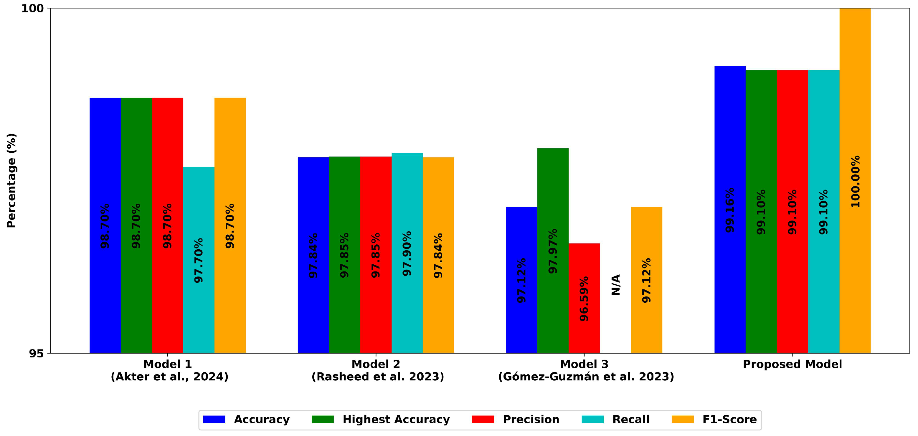
4.2. Model Performance

The model was trained with 57,712 MRI images of four classes: glioma, meningioma, pituitary tumor, and no-tumor. The training process consists of an initial training state and a subsequent fine-tuning stage to enhance the model’s performance. MobilenetV2 with custom preprocessing performs good and has a test accuracy of 99.16%. The high accuracy suggests that the model effectively distinguished its original target, differentiating between four classes of brain tumors.

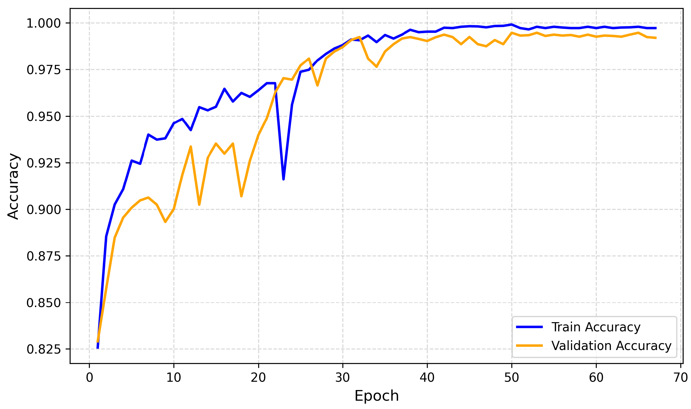
4.2.1. Training and Validation Accuracy

The progression of the training and validation accuracy across all epochs is shown in Figure 9, demonstrating consistent improvement in the model’s ability to classify brain tumor images accurately.

From Figure 9, initially the training accuracy grew sharply, starting at 82.6% in epoch 1 and reaching over 99% accuracy by epoch 40. Similarly, validation accuracy followed a similar upward trend, starting at 83% and peaking at 99% by epoch 46. This consistent improvement indicates that the model successfully generalized its learning to unseen data without overfitting. During the second stage of training, after loosening the frozen layers of the MobileNet base model, the fine-tuned model exhibited rapid performance improvements due to domain-specific adaptation. Validation accuracy during the fine-tuning phase reached its highest value, achieving 98.86%, demonstrating the effectiveness of transfer learning combined with fine-tuning on the MRI dataset.

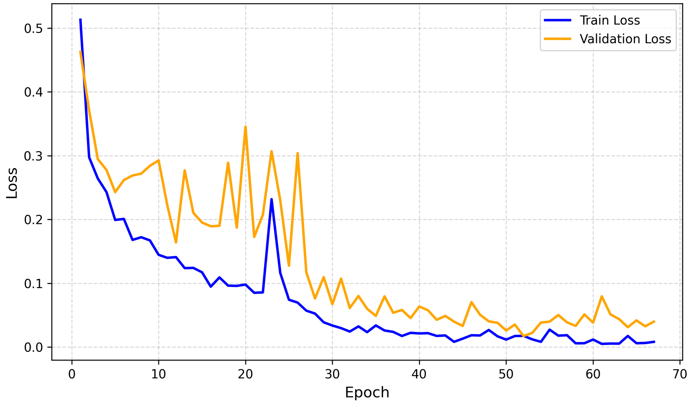
4.2.2. Training and Validation Loss

The model training and validation loss over all epochs is shown in Figure 10, which provides insights into the epochs’ training and validation loss.

From Figure 10, initially, the loss for both training and validation sets decreased significantly. At epoch 1, the training loss was 0.5130, which reduced to less than 0.01 by epoch 40, reflecting optimal convergence of the model. Validation loss also exhibited a declining trend, fluctuating slightly in early epochs, likely due to the variability in the MRI dataset, but stabilizing as epochs progressed. By epoch 46, the validation loss reached 0.0398, confirming that the model achieved strong generalization with minimal overfitting.

The model training consisted of two stages—initial feature extraction followed by fine-tuning. After completing the initial training of 22 epochs with frozen layers, the model began a new training phase, starting from epoch 1, where the last 50 layers of the MobileNet base model were unfrozen for fine-tuning. This technique allowed the model to hone task-specific features while preserving previously learned patterns, resulting in significant performance improvements, particularly on the validation dataset.

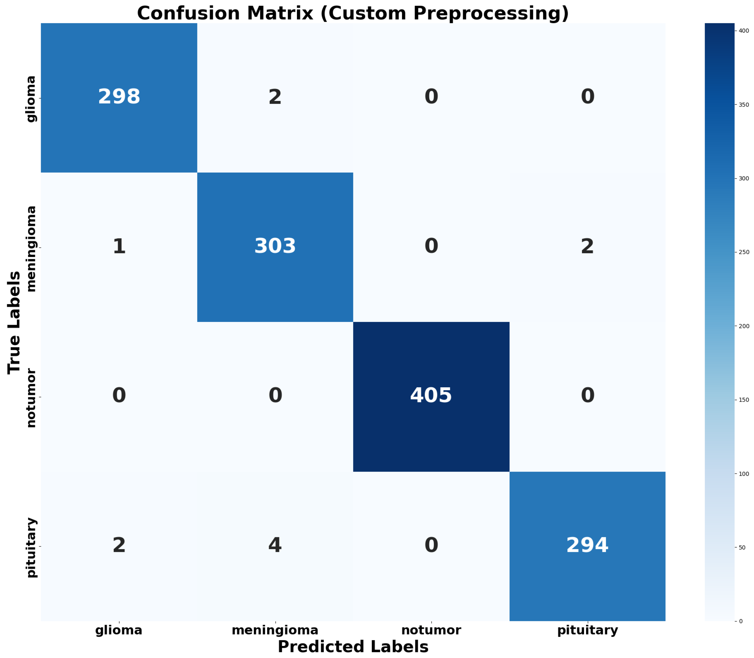
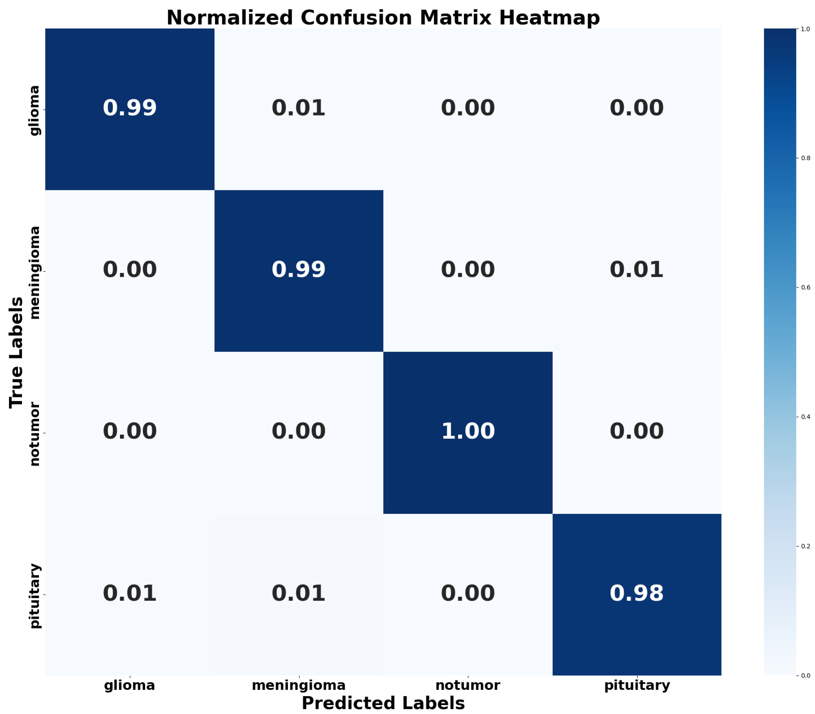
4.2.3. Confusion Matrix and Normalized Confusion Matrix Heatmap

To assess the performance of the proposed brain model, a confusion matrix was computed, the results of which are summarized in Figure 11 and Figure 12. These figures provide a detailed overview of the model’s efficiency in classifying tumors into four categories: Glioma, Meningioma, No Tumor, and Pituitary Tumor.

Figure 11 shows the confusion matrix with actual vs predicted labels for all tumor classes in the test set. The test set comprised 1311 samples, and the model demonstrated strong classification performance with high proportions of correctly classified samples. Notable results as 298 correctly classified samples for Glioma, 303 correctly classified samples for Meningioma, 405 correctly classified samples for No Tumor, and 294 correctly classified samples for Pituitary Tumor. The average performance of the model was strong and demonstrated minimal misclassification while efficiently distinguishing between the four types of tumors.

To aid further analysis, the confusion matrix was normalized, as shown in Figure 12. The normalized confusion matrix measures classification performance as a percentage, enabling improved cross-class comparison. The diagonal values, representing correct classifications, were notably high an Accuracy of 99% for Glioma, Accuracy of 99% for Meningioma, Accuracy of 100% for No Tumor, and Accuracy of 98% for Pituitary Tumor. The off-diagonal values, representing misclassifications, remain exceptionally low, with the largest value being just 1%. This indicates the robustness of the model across all tumor classes, even for tumors with some degree of resemblance. The model demonstrated strong classification performance with a high proportion of correctly classified samples across all tumor types. Notable results included 298 correctly classified samples for Glioma, 303 for Meningioma, 405 for No Tumor, and 294 for Pituitary Tumor. The No Tumor class, despite being a minority class in the dataset, achieved a 100% recall (as seen in the normalized confusion matrix in Figure 12), indicating the absence of false negatives. However, its precision was slightly lower due to 6 misclassified cases distributed across Meningioma and Pituitary Tumor.

Overall, the confusion matrix and its normalized counterpart demonstrate the high precision, recall, and F1 scores achieved by the proposed model. These findings confirm the model’s reliability in classifying brain tumors with minimal error and excellent efficiency in addressing a multi-class classification problem, highlighting its adaptability and robustness.

4.2.4. Learning Rate Curve

The learning rate is an important hyperparameter that directly affects the performance and convergence of neural networks. The learning rate curve, as presented in Figure 13, illustrates how the learning rate is adjusted throughout training for the proposed brain tumor classification model.

From Figure 13, in the initial phases of training, a higher learning rate is preferred; therefore, an initial value of 0.001 was set. This allows the model to make significant weight updates in the initial stages and move closer to the optimal solution. However, as training progresses, higher learning rates can lead to oscillations around the minima or, in some cases, divergence. To address this, a learning rate reduction policy was applied. Specifically, after 10 epochs, the learning rate was reduced to a smaller value, 0.0001, and held constant for the remainder of the training process.

This strategy balances the exploration trade-off: at the beginning of training, the learner explores broader regions of the loss surface, and later it fine-tunes the parameters to converge toward an optimal solution. The flat region of the curve after epoch 10 indicates that the learning process stabilizes, minimizing the risk of overfitting caused by excessive weight adjustments. The learning rate schedule achieves the desired speed of convergence and generalization, as depicted in Figure 13. This step-based reduction technique prevents suboptimal convergence, improves the model’s robustness, and contributes to the high accuracy and reliable performance observed during tumor classification.

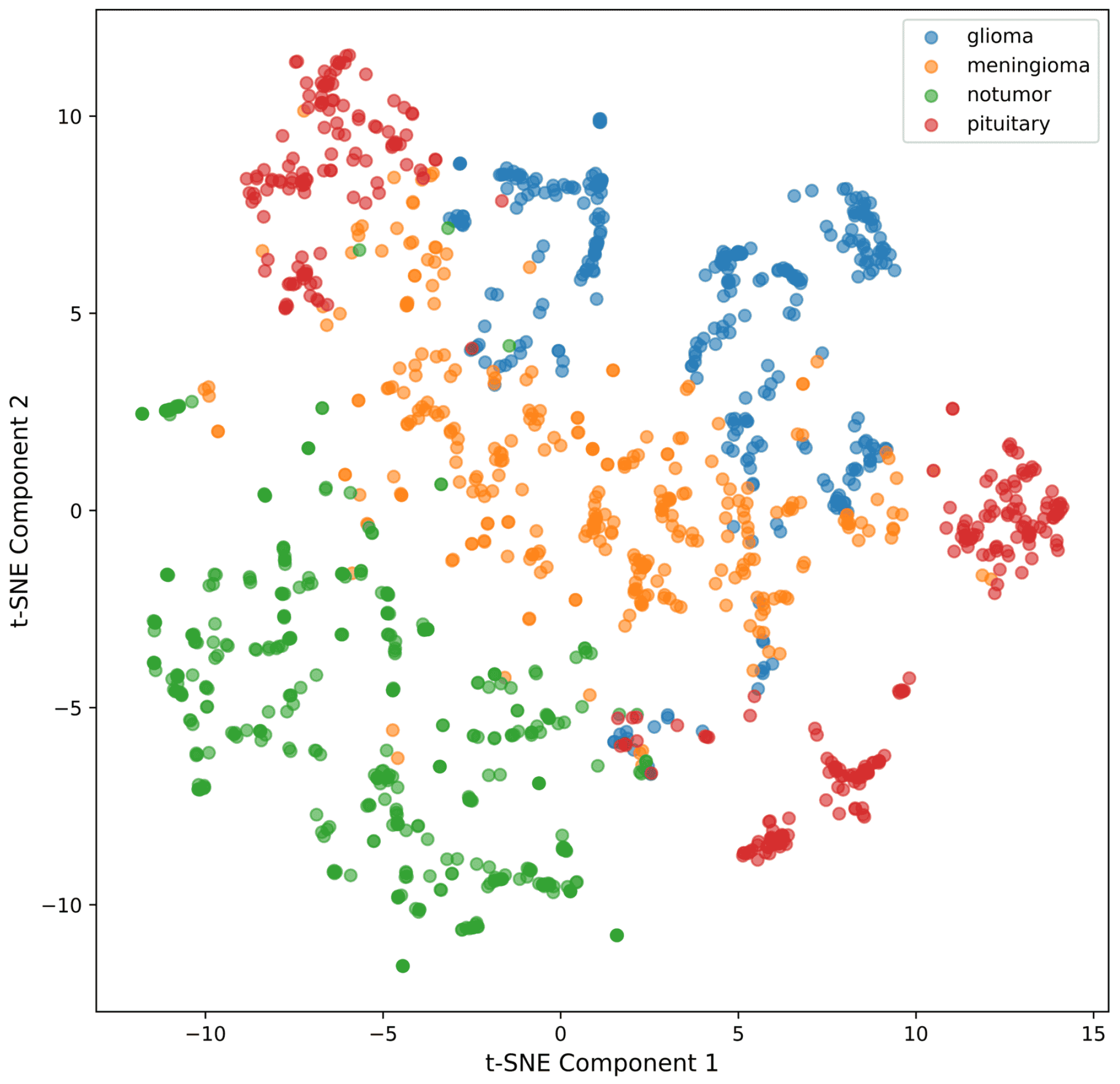
4.2.5. t-SNE for Feature Visualization

To validate the learned feature separations visually, t-SNE was applied to feature embeddings extracted from the final dense layer of the model. This layer captures high-level feature representations before classification, making it a suitable choice for dimensionality reduction and visualization. The t-SNE algorithm was configured with a perplexity of 30, a learning rate of 200, and 1000 iterations to project the high-dimensional feature embeddings into a two-dimensional space. These hyperparameters were chosen to balance the trade-off between local and global feature relationships.

While t-SNE is primarily a visualization tool and may introduce artifacts depending on its configuration, the resulting clusters were consistent with the learned separations for the four tumor classes (glioma, meningioma, pituitary tumor, and no-tumor). This supports the model’s ability to extract meaningful and distinct feature representations. However, we note that t-SNE may distort certain relationships at larger scales, which could be explored further in future work. Figure 14 demonstrates how the model separates the four classes of tumors: Glioma, Meningioma, No Tumor, and Pituitary Tumor.

In the plot, distinct clusters for each class are evident, indicating that the model effectively separates the features. The blue, orange, green, and red clusters correspond respectively to Glioma, Meningioma, No Tumor, and Pituitary Tumor. This demonstrates the model’s ability to discriminate feature representations and achieve optimal classification performance. However, some overlapping clusters at the decision boundaries suggest that the model may face challenges with certain samples due to subtle differences in their feature spaces. The t-SNE visualization further validates that the feature extractor in the proposed model performs as intended. It illustrates how the input data is mapped into a feature space that is not only cohesive but also easily distinguishable, enabling the high classification accuracy achieved in this study. Additionally, this visualization has diagnostic potential by pinpointing spatial areas where misalignments are likely, offering insights for further refinement of the model. Certain areas show potential for further learning and improvement, which could lead to even better results in future iterations.

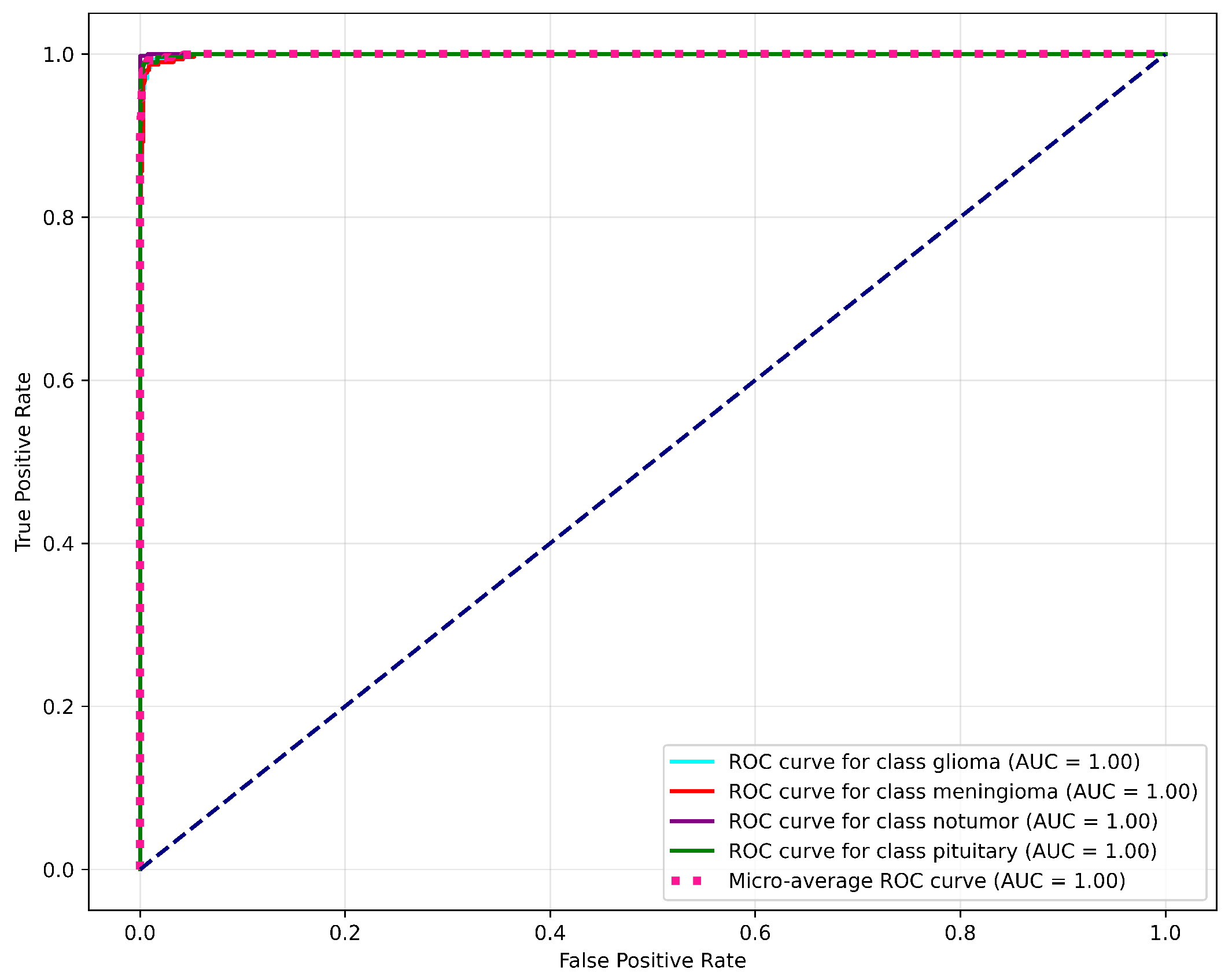
4.2.6. ROC and AUC Curve

The ROC and AUC curves for the different classes of the brain tumor classification model are illustrated in Figure 15, along with the micro-average ROC curve.

From Figure 15, the plot simultaneously shows the Receiver Operating Characteristic (ROC) curve, highlighting the relationship between the True Positive Rate (TPR), Area Under the Curve (AUC), and the False Positive Rate (FPR) across varying thresholds. Additionally, the plot includes:

• Specific ROC Classes: A separate sub-plot for each class, containing the ROC curve for glioma, meningioma, pituitary tumor, and no tumor, along with their respective AUC values. The model achieves an AUC of 1.00 for each tumor class, which indicates its superior performance.
• Micro-Average ROC Curve: A single curve that aggregates the performance of the model across all classes to yield a micro-average AUC of 1.00.
• Random Guessing Line: A dashed diagonal line with an AUC of 0.50, representing random guessing. The position of this line helps in understanding the model’s ability to distinguish between the different classes.

The AUC scores for all tumor classes (glioma, meningioma, pituitary tumor, and no tumor) demonstrate the model’s robustness and discriminatory power in the multi-class setup. This visualization, combined with the data, confirms that the pre-trained MobileNetV2 architecture, paired with fine-tuning strategies and custom pre-processing methods, significantly improves classification outcomes.

4.2.7. Model Execution Time Analysis

The time utilized by the proposed model for classifying brain tumors was analyzed to determine its efficiency during both training and inference. The computations, as summarized below, highlight that the model was able to maintain high performance metrics while achieving a balanced computation time. The model underwent training for ten epochs, with each epoch taking between 97 to 115 s, depending on the complexity of gradient updates and the data processing involved. In total, the complete training process lasted for 1019.75 s (or approximately 17 min), with an average duration of 102 s per epoch. The accuracy and loss metrics from both training and validation indicate rapid convergence, showcasing that the computational demands were met effectively.

During testing, the model achieved an evaluation time of 8.57 s across 41 batches, averaging 199 ms per step. Such a swift inference time demonstrates the model’s capability for real-time or near-real-time applications, such as medical imaging diagnostics, where quick predictions are crucial. The overall execution times for training and inference emphasize the computational efficiency of the proposed model. Additionally, its ability to deliver high accuracy and robustness highlights its practical applicability for real-world clinical scenarios, making it a reliable tool for brain tumor classification.

4.3. Error Analysis

As observed in the confusion matrix, there are very few misclassifications of classes, which highlights the robustness of the proposed model. However, the following errors can still be noted:

• Glioma Misclassifications: 2 Meningioma instances were misclassified as Glioma.
• Meningioma Misclassifications: 2 samples of Pituitary Tumor were predicted to be Meningioma.
• Other Misclassifications: 1 sample of Glioma, 4 Meningioma, and 2 Pituitary Tumor samples were classified as the remaining classes.
• Class Distribution and Imbalance Analysis: The pre-partitioned distribution of the dataset reveals that the No Tumor class is a majority class, comprising 27.9% of the training data and 30.9% of the testing data. On the other hand, the Glioma and Pituitary Tumor classes have lower representation in both subsets, each contributing fewer overall images in comparison. This discrepancy created a slight class imbalance that could potentially bias the training process. 2 misclassifications as Meningioma, 4 misclassifications as Pituitary Tumor.

These errors appear to have been caused by overlapping characteristics between certain tumor types or subtle details within the dataset. Despite such a small number of errors, the classification accuracy remains highly reliable, as the high diagonal values in the confusion matrix offset the impact of the few off-diagonal metrics. Further improvement in feature extraction techniques or the inclusion of additional data could help mitigate these minor identification errors.

Result Analysis and Comparative Evaluation The accuracy results obtained from this study show that the application of a preprocessing filter in combination with the MobileNetV2 architecture improves accuracy in classifying brain tumors. The model proposed in this paper has an accuracy of 99.16%, which is remarkable, considering the traditional and even modern advanced methods. Estimates obtained from the confusion matrix indicate strong precision, recall, and F1-scores for all classes with very low rates of misclassification. The symmetry in sensitivity (true positive rates) and specificity (the rate of correctly identified non-cases) further strengthens the balance offered by the proposed model. Assessments and observations made during training and validation cycles show that loss values were low without overfitting, and the convergence exhibited smooth gradients, indicating optimization techniques were proficient.

With fine-tuning of MobileNetV2, the model was able to adjust successfully to new datasets, which shows its usefulness in real-life applications. The use of more advanced data augmentation methods, along with better preprocessing, ensured that the model maintained accuracy and flexibility when applied to unseen data. This adaptability and accuracy emphasize the great promise of MobileNetV2 in assisting radiologists during real-time diagnosis and treatment of brain tumor patients. The ability to identify four tumor types, which include Glioma, Meningioma, No-tumor, and Pituitary tumor, makes it invaluable for specific medical practices that are sensitive to misclassification errors.

When measured against other methods, the results of the MobileNetV2 approach were the best. For example, U-Net-based segmentation had a lower accuracy, which was 98.8%, while our technique exceeded it by 0.36%. This demonstrates how fine-tuning MobileNetV2 benefits the task. This proves that MobileNetV2 with proper training and fine-tuning is a good option for brain tumor classification. Likewise, this research also surpassed the accuracy of a previous CNN-based automated tumor image categorization method reported in [43]. Another comparison was made with reference [44] who implemented modern CNN methods and reported 97.84% accuracy. The results of our method were a 1.32% enhancement from this while also keeping the cost in terms of computation low due to MobileNetV2’s light weight.

Moreover, MobileNetV2 architecture is superior when placed alongside other models such as InceptionV3, which only achieved 97.12% [41], and that is MobileNetV2’s strongest feature—its 2.04% increase in accuracy yields awesome results in classifying various tumor images, which ensures correct predictions and reduces errors. With this accuracy and reliability, the MobileNetV2 model becomes not only an alternative but a dependable model for early diagnosis and clinical decision making. The study also shows that simplistic neural networks integrated with sophisticated preprocessing techniques can outperform their more powerful counterparts, which gives a more elegant and scalable answer for medical practitioners.

Overall, the optical flow results proved the efficiency of the suggested methods that were based on the MobileNetV2 architecture. The integration of reliable preprocessing steps with a deep learning model has made it possible for the proposed method to predominantly excel in brain tumor classification tasks, beating the load of other models that are already well known because of their accuracy and efficiency.

5. Conclusions

This study highlights the effectiveness of a MobileNetV2-based framework for brain tumor classification using MRI images, achieving state-of-the-art accuracy while maintaining computational efficiency. Through the integration of advanced preprocessing techniques, transfer learning, and fine-tuned configurations, the model successfully classified glioma, meningioma, pituitary tumor, and no tumor with remarkable precision. These results validate the method’s potential to serve as a reliable decision-support tool in medical applications. Though the results vary from the previous research not much than 1% to 2%, but this slight improvement will have a great impact in real life implimentation. The proposed preprocessing pipeline enhances the model’s ability to generalize across varied MRI images, even under noise or variability, ensuring reliable performance in clinical scenarios.

The research, however, has certain limitations that warrant further investigation. The use of a predefined dataset split limits the evaluation of model generalizability, as no cross-validation or independent validation sets were employed with different dataset. Additionally, the dataset’s limited scope and diversity, primarily originating from a single source, may not fully reflect the variability seen in real-world clinical imaging conditions. Clinical integration concerns, such as interpretability, scalability, and workflow compatibility, remain unaddressed and require future attention. Furthermore, the near-perfect performance metrics signal a potential susceptibility to overfitting, highlighting the need for validation on larger, more diverse datasets to confirm reliability.

To address these limitations, future work will prioritize incorporating cross-validation techniques to comprehensively assess performance variability. Expanding the dataset to include images from various institutions, imaging protocols, and patient demographics will enhance the model’s generalizability. Systematic optimization of transfer learning strategies, including exploring alternative architectures such as EfficientNet or ensemble-based methods, will further improve classification accuracy and computational efficiency. Real-world testing in clinical environments is essential to evaluate the model’s utility in practice while addressing critical factors such as interpretability, privacy concerns, and seamless integration with existing workflows.

In summary, the proposed approach represents a significant step forward in using deep learning for brain tumor classification. By addressing its limitations and expanding its scope through future enhancements, this research can contribute meaningfully to improving diagnostic accuracy, reducing the workload for healthcare professionals, and ultimately enhancing outcomes in clinical care. We believe the findings of this study lay a strong foundation for further advancements in the field and demonstrate potential for impactful applications in medical practice.

References

1. Sriharikrishnaa, S.; Suresh, P.S.; Prasada, K.S. An introduction to fundamentals of cancer biology. In Optical Polarimetric Modalities for Biomedical Research; Springer: Berlin/Heidelberg, Germany, 2023; pp. 307–330. [Google Scholar]
2. Razzak, M.I.; Imran, M.; Xu, G. Efficient brain tumor segmentation with multiscale two-pathway-group conventional neural networks. IEEE J. Biomed. Health Inform. 2018, 23, 1911–1919. [Google Scholar] [CrossRef] [PubMed]
3. Lei, B.; Yang, P.; Zhuo, Y.; Zhou, F.; Ni, D.; Chen, S.; Xiao, X.; Wang, T. Neuroimaging retrieval via adaptive ensemble manifold learning for brain disease diagnosis. IEEE J. Biomed. Health Inform. 2018, 23, 1661–1673. [Google Scholar] [CrossRef] [PubMed]
4. Mikhno, A.; Zanderigo, F.; Ogden, R.T.; Mann, J.J.; Angelini, E.D.; Laine, A.F.; Parsey, R.V. Toward noninvasive quantification of brain radioligand binding by combining electronic health records and dynamic PET imaging data. IEEE J. Biomed. Health Inform. 2015, 19, 1271–1282. [Google Scholar] [CrossRef]
5. Abiwinanda, N.; Hanif, M.; Hesaputra, S.T.; Handayani, A.; Mengko, T.R. Brain tumor classification using convolutional neural network. In Proceedings of the World Congress on Medical Physics and Biomedical Engineering 2018, Prague, Czech Republic, 3–8 June 2018; Springer: Berlin/Heidelberg, Germany, 2019; Volume 1, pp. 183–189. [Google Scholar]
6. Ghasemi, N.; Razavi, S.; Nikzad, E. Multiple sclerosis: Pathogenesis, symptoms, diagnoses and cell-based therapy. Cell J. 2017, 19, 1. [Google Scholar] [PubMed]
7. ZainEldin, H.; Gamel, S.A.; El-Kenawy, E.S.M.; Alharbi, A.H.; Khafaga, D.S.; Ibrahim, A.; Talaat, F.M. Brain tumor detection and classification using deep learning and sine-cosine fitness grey wolf optimization. Bioengineering 2022, 10, 18. [Google Scholar] [CrossRef]
8. Del Dosso, A.; Urenda, J.P.; Nguyen, T.; Quadrato, G. Upgrading the physiological relevance of human brain organoids. Neuron 2020, 107, 1014–1028. [Google Scholar] [CrossRef]
9. Amin, J.; Sharif, M.; Haldorai, A.; Yasmin, M.; Nayak, R.S. Brain tumor detection and classification using machine learning: A comprehensive survey. Complex Intell. Syst. 2022, 8, 3161–3183. [Google Scholar] [CrossRef]
10. Gritsch, S.; Batchelor, T.T.; Gonzalez Castro, L.N. Diagnostic, therapeutic, and prognostic implications of the 2021 World Health Organization classification of tumors of the central nervous system. Cancer 2022, 128, 47–58. [Google Scholar] [CrossRef]
11. Louis, D.N.; Perry, A.; Wesseling, P.; Brat, D.J.; Cree, I.A.; Figarella-Branger, D.; Hawkins, C.; Ng, H.; Pfister, S.M.; Reifenberger, G.; et al. The 2021 WHO classification of tumors of the central nervous system: A summary. Neuro-oncology 2021, 23, 1231–1251. [Google Scholar] [CrossRef]
12. Fountain, D.M.; Soon, W.C.; Matys, T.; Guilfoyle, M.R.; Kirollos, R.; Santarius, T. Volumetric growth rates of meningioma and its correlation with histological diagnosis and clinical outcome: A systematic review. Acta Neurochir. 2017, 159, 435–445. [Google Scholar] [CrossRef]
13. Miah, M.B.A.; Kana, K.A.; Akter, A. Detection of brain cancer from MRI images using neural network. Int. J. Appl. Inf. Syst. 2016, 10, 6–11. [Google Scholar]
14. Kleihues, P.; Soylemezoglu, F.; Schäuble, B.; Scheithauer, B.W.; Burger, P.C. Histopathology, classification, and grading of gliomas. Glia 1995, 15, 211–221. [Google Scholar] [CrossRef] [PubMed]
15. Ohgaki, H.; Kleihues, P. Epidemiology and etiology of gliomas. Acta Neuropathol. 2005, 109, 93–108. [Google Scholar] [CrossRef] [PubMed]
16. Alruwaili, A.A.; De Jesus, O. Meningioma, updated 2023 aug 23 ed.; StatPearls Publishing: Treasure Island, FL, USA, 2024. [Google Scholar]
17. Melmed, S. Pathogenesis of pituitary tumors. Nat. Rev. Endocrinol. 2011, 7, 257–266. [Google Scholar] [CrossRef] [PubMed]
18. Zakareya, M.; Alam, M.B.; Ullah, M.A. Classification of cancerous skin using artificial neural network classifier. Int. J. Comput. Appl. 2018, 975, 8887. [Google Scholar] [CrossRef]
19. Miah, M.B.A.; Yousuf, M.A. Detection of lung cancer from CT image using image processing and neural network. In Proceedings of the 2015 International Conference on Electrical Engineering and Information Communication Technology (ICEEICT), Savar, Dhaka, Bangladesh, 21–23 May 2015; pp. 1–6. [Google Scholar]
20. Raghuvanshi, S.; Dhariwal, S. The VGG16 Method Is a Powerful Tool for Detecting Brain Tumors Using Deep Learning Techniques. Eng. Proc. 2023, 59, 46. [Google Scholar]
21. Mahmud, M.I.; Mamun, M.; Abdelgawad, A. A deep analysis of brain tumor detection from mr images using deep learning networks. Algorithms 2023, 16, 176. [Google Scholar] [CrossRef]
22. Chan, H.P.; Samala, R.K.; Hadjiiski, L.M.; Zhou, C. Deep learning in medical image analysis. In Deep Learning in Medical Image Analysis: Challenges and Applications; Springer Nature: Cham, Switzerland, 2020; pp. 3–21. [Google Scholar]
23. Elaissaoui, K.; Ridouani, M. Application of Deep Learning in Healthcare: A Survey on Brain Tumor Detection. ITM Web Conf. 2023, 52, 02005. [Google Scholar] [CrossRef]
24. Methil, A.S. Brain tumor detection using deep learning and image processing. In Proceedings of the 2021 International Conference on Artificial Intelligence and Smart Systems (ICAIS), Coimbatore, India, 25–27 March 2021; pp. 100–108. [Google Scholar]
25. Kumar, P.R.; Bonthu, K.; Meghana, B.; Vani, K.S.; Chakrabarti, P. Multi-class Brain Tumor Classification and Segmentation using Hybrid Deep Learning Network Model. Scalable Comput. Pract. Exp. 2023, 24, 69–80. [Google Scholar] [CrossRef]
26. Wadhwa, A.; Bhardwaj, A.; Verma, V.S. A review on brain tumor segmentation of MRI images. Magn. Reson. Imaging 2019, 61, 247–259. [Google Scholar] [CrossRef]
27. Jesmin, T.; Ahmed, K.; Rahman, M.; Miah, M. Brain cancer risk prediction tool using data mining. Int. J. Comput. Appl. 2013, 61, 12. [Google Scholar] [CrossRef]
28. Tan, M.; Le, Q. Efficientnet: Rethinking model scaling for convolutional neural networks. In Proceedings of the International Conference on Machine Learning, PMLR, Long Beach, CA, USA, 9–15 June 2019; pp. 6105–6114. [Google Scholar]
29. Ma, N.; Zhang, X.; Zheng, H.T.; Sun, J. Shufflenet v2: Practical guidelines for efficient cnn architecture design. In Proceedings of the European Conference on Computer Vision (ECCV), Munich, Germany, 8–14 September 2018; pp. 116–131. [Google Scholar]
30. Ghadi, N.M.; Salman, N.H. Deep learning-based segmentation and classification techniques for brain tumor MRI: A review. J. Eng. 2022, 28, 93–112. [Google Scholar] [CrossRef]
31. Patil, S.; Kirange, D. Ensemble of deep learning models for brain tumor detection. Procedia Comput. Sci. 2023, 218, 2468–2479. [Google Scholar] [CrossRef]
32. Akkus, Z.; Galimzianova, A.; Hoogi, A.; Rubin, D.L.; Erickson, B.J. Deep learning for brain MRI segmentation: State of the art and future directions. J. Digit. Imaging 2017, 30, 449–459. [Google Scholar] [CrossRef]
33. Younis, A.; Qiang, L.; Nyatega, C.O.; Adamu, M.J.; Kawuwa, H.B. Brain tumor analysis using deep learning and VGG-16 ensembling learning approaches. Appl. Sci. 2022, 12, 7282. [Google Scholar] [CrossRef]
34. Jiang, Z.; Ding, C.; Liu, M.; Tao, D. Two-stage cascaded u-net: 1st place solution to brats challenge 2019 segmentation task. In Brainlesion: Glioma, Multiple Sclerosis, Stroke and Traumatic Brain Injuries, Proceedings of the 5th International Workshop, BrainLes 2019, Held in Conjunction with MICCAI 2019, Shenzhen, China, 17 October 2019; Revised Selected Papers, Part I 5; Springer: Berlin/Heidelberg, Germany, 2020; pp. 231–241. [Google Scholar]
35. Aboelenein, N.M.; Songhao, P.; Koubaa, A.; Noor, A.; Afifi, A. HTTU-Net: Hybrid Two Track U-Net for automatic brain tumor segmentation. IEEE Access 2020, 8, 101406–101415. [Google Scholar] [CrossRef]
36. Kang, J.; Ullah, Z.; Gwak, J. MRI-based brain tumor classification using ensemble of deep features and machine learning classifiers. Sensors 2021, 21, 2222. [Google Scholar] [CrossRef] [PubMed]
37. Sleem; Metwaly, A.A. A deep learning-based model for evaluating academic performance using student behavior patterns. Sustain. Mach. Intell. J. 2023, 3, 1–10. [Google Scholar]
38. Tolba; Fathy. Chaotic metaheuristic optimization for improving text classification performance. Sustain. Mach. Intell. J. 2023, 3, 1–10. [Google Scholar]
39. Celik, M.; Inik, O. Development of hybrid models based on deep learning and optimized machine learning algorithms for brain tumor Multi-Classification. Expert Syst. Appl. 2024, 238, 122159. [Google Scholar] [CrossRef]
40. Srinivas, C.; KS, N.P.; Zakariah, M.; Alothaibi, Y.A.; Shaukat, K.; Partibane, B.; Awal, H. Deep transfer learning approaches in performance analysis of brain tumor classification using MRI images. J. Healthc. Eng. 2022, 2022, 3264367. [Google Scholar] [CrossRef] [PubMed]
41. Gómez-Guzmán, M.A.; Jiménez-Beristaín, L.; García-Guerrero, E.E.; López-Bonilla, O.R.; Tamayo-Perez, U.J.; Esqueda-Elizondo, J.J.; Palomino-Vizcaino, K.; Inzunza-González, E. Classifying brain tumors on magnetic resonance imaging by using convolutional neural networks. Electronics 2023, 12, 955. [Google Scholar] [CrossRef]
42. Kazemi, A.; Shiri, M.E.; Sheikhahmadi, A. Classifying tumor brain images using parallel deep learning algorithms. Comput. Biol. Med. 2022, 148, 105775. [Google Scholar] [CrossRef] [PubMed]
43. Akter, A.; Nosheen, N.; Ahmed, S.; Hossain, M.; Yousuf, M.A.; Almoyad, M.A.A.; Hasan, K.F.; Moni, M.A. Robust clinical applicable CNN and U-Net based algorithm for MRI classification and segmentation for brain tumor. Expert Syst. Appl. 2024, 238, 122347. [Google Scholar] [CrossRef]
44. Rasheed, Z.; Ma, Y.K.; Ullah, I.; Ghadi, Y.Y.; Khan, M.Z.; Khan, M.A.; Abdusalomov, A.; Alqahtani, F.; Shehata, A.M. Brain tumor classification from MRI using image enhancement and convolutional neural network techniques. Brain Sci. 2023, 13, 1320. [Google Scholar] [CrossRef]
45. Nickparvar, M. Brain Tumor MRI Dataset. 2021. Available online: https://www.kaggle.com/datasets/masoudnickparvar/brain-tumor-mri-dataset (accessed on 22 May 2025).
46. Cheng, J. Brain Tumor Dataset. 2017. Available online: https://figshare.com/articles/dataset/brain_tumor_dataset/1512427/5 (accessed on 22 May 2025).
47. Hamada, A. Brain Tumor Detection. 2022. Available online: https://www.kaggle.com/datasets/ahmedhamada0/brain-tumor-detection (accessed on 22 May 2025).
48. Setiawan, A.W.; Mengko, T.R.; Santoso, O.S.; Suksmono, A.B. Color retinal image enhancement using CLAHE. In Proceedings of the International Conference on ICT for Smart Society, Jakarta, Indonesia, 13–14 June 2013; pp. 1–3. [Google Scholar]
49. Miah, M.B.A.; Awang, S.; Azad, M.S.; Rahman, M.M. Keyphrases concentrated area identification from academic articles as feature of keyphrase extraction: A new unsupervised approach. Int. J. Adv. Comput. Sci. Appl. 2022, 13, 789–796. [Google Scholar] [CrossRef]
50. Miah, M.B.A.; Awang, S.; Rahman, M.M.; Hosen, A.S.; Ra, I.H. Keyphrases frequency analysis from research articles: A region-based unsupervised novel approach. IEEE Access 2022, 10, 120838–120849. [Google Scholar] [CrossRef]
51. Xie, J.; Wu, J.; Xiao, Z. Spatio-Temporal Patterns and Sentiment Analysis of Ting, Tai, Lou, and Ge Ancient Chinese Architecture Buildings. Buildings 2025, 15, 1652. [Google Scholar] [CrossRef]
52. Chicco, D.; Tötsch, N.; Jurman, G. The Matthews correlation coefficient (MCC) is more reliable than balanced accuracy, bookmaker informedness, and markedness in two-class confusion matrix evaluation. BioData Min. 2021, 14, 19. [Google Scholar] [CrossRef]
53. Chicco, D.; Warrens, M.J.; Jurman, G. The Matthews correlation coefficient (MCC) is more informative than Cohen’s Kappa and Brier score in binary classification assessment. IEEE Access 2021, 9, 78368–78381. [Google Scholar] [CrossRef]
54. Sherif, M.M. Brain Tumor Dataset. 2022. Available online: https://www.kaggle.com/datasets/mohamedmetwalysherif/braintumordataset (accessed on 22 May 2025).
55. Kumar, P. Brain MRI. 2021. Available online: https://www.kaggle.com/datasets/pradeep2665/brain-mri (accessed on 22 May 2025).
56. Chakrabarty, N. Brain MRI Images for Brain Tumor Detection. Dataset Used in the Study “Brain Tumor Analysis Using Deep Learning and VGG-16 Ensembling Learning Approaches.”. 2022. Available online: https://www.kaggle.com/datasets/navoneel/brain-mri-images-for-brain-tumor-detection (accessed on 25 June 2024).
Figure 1. Four(4) types of MRI images of brain tumor.
Biomedinformatics 05 00030 g001
Figure 2. Several steps of image prepossessing techniques.
Biomedinformatics 05 00030 g002
Figure 3. Original MRI images and preprocessed final images for each tumor class.
Biomedinformatics 05 00030 g003
Figure 4. Functional details of the basic MobileNetv2 architecture.
Biomedinformatics 05 00030 g004
Figure 5. Detailed overview of the MobilenetV2 architecture.
Biomedinformatics 05 00030 g005
Figure 6. Overview of fine-tuning MobilenetV2 (proposed model).
Biomedinformatics 05 00030 g006
Figure 7. Technical architecture of fine-tuning MobilenetV2 (proposed model).
Biomedinformatics 05 00030 g007
Figure 8. Comparison of brain tumor classification models with different evaluation matrix [41,43,44].
Biomedinformatics 05 00030 g008
Figure 9. Training and validation accuracy over all epochs.
Biomedinformatics 05 00030 g009
Figure 10. Training and validation loss over all epochs.
Biomedinformatics 05 00030 g010
Figure 11. Confusion matrix of the model.
Biomedinformatics 05 00030 g011
Figure 12. Normalized confusion matrix heatmap of the model.
Biomedinformatics 05 00030 g012
Figure 13. The learning rate curve for training the proposed model.
Biomedinformatics 05 00030 g013
Figure 14. t-SNE features for dimensionality reduction and visualization.
Biomedinformatics 05 00030 g014
Figure 15. ROC and AUC curve for each class.
Biomedinformatics 05 00030 g015