Abstract
Background: This work presents an artificial intelligence-based algorithm for detecting Parkinson’s disease (PD) from voice signals. The detection of PD at pre-symptomatic stages is imperative to slow disease progression. Speech signal processing-based PD detection can play a crucial role here, as it has been reported in the literature that PD affects the voice quality of patients at an early stage. Hence, speech samples can be used as biomarkers of PD, provided that suitable voice features and artificial intelligence algorithms are employed. Methods: Advanced signal-processing techniques are used to extract audio features from the sustained vowel ‘/a/’ sound. The extracted audio features include baseline features, intensities, formant frequencies, bandwidths, vocal fold parameters, and Mel-frequency cepstral coefficients (MFCCs) to form a feature vector. Then, this feature vector is further enriched by including wavelet-based features to form the second feature vector. For classification purposes, two popular machine learning models, namely, support vector machine (SVM) and k-nearest neighbors (kNNs), are trained to distinguish patients with PD. Results: The results demonstrate that the inclusion of wavelet-based voice features enhances the performance of both the SVM and kNN models for PD detection. However, kNN provides better accuracy, detection speed, training time, and misclassification cost than SVM. Conclusions: This work concludes that wavelet-based voice features are important for detecting neurodegenerative diseases like PD. These wavelet features can enhance the classification performance of machine learning models. This work also concludes that kNN is recommendable over SVM for the investigated voice features, despite the inclusion and exclusion of the wavelet features.
1. Introduction
The number of patients with Parkinson’s disease (PD) has increased at an unprecedented rate with the increase in life expectancy of humans. The American Association of Neurosurgeons (AAN) reports sixty thousand new PD cases each year in the USA alone. Currently, 1.5 million Americans suffer from this disease [1]. Global statistics are even more alarming; a recent publication by the World Health Organization (WHO) shows that the number of patients with PD has doubled over the past 25 years [2].
Parkinson first reported this disease in his investigative work [3]. PD is caused by the degeneration of nerve cells in the substantia nigra of the brain. These brain nerve cells do not produce the required ‘dopamine’. Studies have confirmed that symptoms of PD develop in patients after 80% or greater loss of dopamine-producing cells in the substantia nigra [1]. Dopamine, with the help of neurotransmitters, coordinates millions of nerve and muscle cells involved in the movement of body parts. Insufficient dopamine production results in impaired movement and other symptoms [4]. The causes of the variant PD remain an enigma and are currently under investigation. Many theories are still evolving to determine the real causes of PD [2].
Six neuropathologic stages of PD have been reported during the evolution of this disease [5]. Olfactory and vocal disorders appear in the first two stages of the disease. During the third and fourth stages, motor symptoms become more apparent, facilitating the diagnosis of PD by expert physicians. Large brain areas are severely affected in the fifth and sixth stages. Patients lose their self-dependency in movement and other day-to-day activities in these last two stages.
Voice disorders in early-stage PD patients occur due to impairments in the patients’ voice generation system (Figure 1). The results of these impairments may include defective utterance of voice [6], reduced volume, reduced pitch range, and difficulty in articulating sounds [7]. Patients with PD slur and pause while speaking. In addition, the speech of patients with PD becomes monotonic. Generally, a combination of several of the symptoms mentioned above can raise suspicion of early-stage PD. It has been reported that patients with PD suffer from voice disorders [8]. Researchers have also reported similar findings in another survey [9].
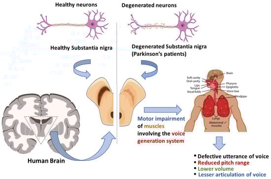
Figure 1.
The progression of voice impairment in patients with Parkinson’s disease.
Detecting PD at pre-symptomatic stages (i.e., stage 1 or 2) is imperative, as the required treatment at the early stage of PD can prevent subsequent neural loss in the substantia nigra and, hence, can slow down disease progression. Speech sample-based PD detection can play a crucial role in this context. Voice sample-based PD detection has several advantages: (a) it is a non-invasive method of PD detection; (b) the voice of PD patients can be easily recorded and analyzed; (c) advanced signal-processing techniques can be applied to extract useful voice features; (d) existing healthcare systems can be easily integrated to detect PD from a remote location despite the visit to healthcare centers; (e) the classification of voice features can be performed using cutting-edge artificial intelligence algorithms; and (f) early detection of PD and the required medical care might improve the quality of the patient’s life.
2. Related Works
Vowel sounds, speech samples, and running speeches have been used to detect certain diseases [10,11], including PD. In [12], the authors collected voice samples from 31 patients (with and without PD). They extracted 22 features from voice samples to form feature vectors. Three machine learning algorithms were modeled to perform detection tasks. The authors achieved the highest accuracy (i.e., 93.82%) using the kNN algorithm.
Pitch period entropy (PPE) was introduced in [13] to detect PD. The authors claimed that PPE is robust against uncontrollable noise and is particularly suitable for telemonitoring applications of PD patients with PD. Sustained phonation from 31 patients, including 23 patients with PD, was adopted for the investigation. The authors concluded that non-standard methods, combined with the traditional harmonics-to-noise ratio (HNR), can best discriminate PD samples from healthy subjects.
To detect PD, the authors employed an artificial neural network (ANN) and voice features [14]. They extracted 44 audio features from the vowel ‘/a/’ sounds. They modeled a feed-forward neural network (FFNN) for classification. They claimed that the proposed two-layered approach can avoid an overwhelming computational burden compared with other deep learning-based systems. The proposed algorithm achieved a high accuracy of 85%.
A remote PD patient monitoring system was proposed in [15]. The system uses a scale called UPDRS (Unified Parkinson’s Disease Rating Scale) to monitor disease progression in patients with PD. The main advantage of their proposed system is that patients do not need to visit a healthcare facility; hence, it is convenient for patients and medical staff. The authors also presented a robust feature-selection algorithm in their work.
Voice features and four classifiers were used in [16] to detect PD. The authors used SVM, kNN, multilayer perceptron, and random forest (RF) as classifiers. They considered gender-based, balanced, and unbalanced datasets in their investigation. The authors investigated four groups of voice features: baseline features, Mel-frequency cepstral coefficients (MFCC), wavelet transform (WT)-based features, and tunable Q-factor wavelet transform (TQWT)-based features. They achieved a detection accuracy of 95.9%, sensitivity of 98.35%, specificity of 91.06%, and precision of 95.6% in female samples. In contrast, they also achieved an accuracy of 94.36%, sensitivity of 100%, specificity of 97.1%, and precision of 96.83% in male samples. The authors also concluded that the high-frequency components of the voice samples provide the most significant functional information to assist in PD detection in female samples. In contrast, low-frequency content assists in PD detection in male samples.
The TQWT was also investigated in [17]. The authors claimed that the TQWT is more effective than the classical discrete-time wavelet transform (DTWT) because it provides a higher frequency resolution of voice signals. The authors used voice recordings from 252 subjects in their investigation. The results show that TQWT performs better than other state-of-the-art speech signal-processing techniques in PD classification. The results also show that the combination of MFCC and TQWT provides the highest accuracy.
In [18], the authors claimed that the misdiagnosis rate of PD detection systems reported in the literature is remarkably high (i.e., 25%), and machine learning-based algorithms can reduce this misdiagnosis rate. The authors proposed AI-based PD detection techniques employing four different classifiers: neural networks (NNs), DMNeural, regression, and decision trees. According to their results, NNs yielded the best results. The authors achieved an overall classification accuracy of 92.9%.
A genetic algorithm-based PD detection model was presented in [19]. The authors claimed that 90% of people with PD suffer from speech and voice disorders and that speech samples can be used to detect PD. The authors extracted various features from the voice signals and detected the optimized features by applying a genetic algorithm. The optimized features were then applied to kNN to classify the samples. The author achieved classification accuracies of 93.7%, 94.8%, and 98.2% using four, seven, and nine optimized features.
Another significant work was presented in [20] to detect PD. The proposed diagnosis method consists of two main steps: feature selection and classification process. The authors employed feature importance and recursive feature elimination methods to select optimized features. They employed three machine learning algorithms, namely, classification and regression trees, ANN, and SVM, for classification. The authors achieved the highest accuracy of 93.84% using SVM with the recursive feature elimination method. A decision support system was presented in [21] to aid specialists in diagnosing PD. The authors used ANN and SVM to detect PD. The authors tested their algorithms on 31 patients and achieved a high accuracy of 90%.
Principal component analysis (PCA) and linear discriminant analysis (LDA) were used in [22] to detect PD. The authors used a speech feature dataset extracted from 252 subjects. PCA and LDA integrate highly correlated features. The authors employed ensemble classifiers in their works. The experimental results show that PCA performs better than LDA. The prediction results indicated that these boosting classifiers provide higher accuracy than the bagging classifiers.
In a similar work [23], various machine-learning models were employed for PD detection. The authors used two feature-selection techniques, namely, mRMR (minimum-redundancy and maximum-relevance) and RFE (recursive feature elimination). The results showed that XGBoost outperforms the other classifiers. The authors achieved an accuracy of 92.76% by adopting the RFE feature-selection technique. Conversely, they achieved an accuracy of 95.39% by employing the mRMR feature-selection technique.
A novel multiple-feature evaluation approach (MFEA) for a multi-agent system was presented in [24] to detect PD. The authors implemented five independent classifiers, namely decision tree, Naïve Bayes, neural network, random forests, and SVM, for diagnosing Parkinson’s disease. They investigated the performance of these machine learning algorithms with and without MFEA. The test results show that the MFEA of the multi-agent system improved the performance of the decision tree, Naïve Bayes, neural network, random forest, and SVM by 10.51%, 15.22%, 9.19%, 12.75%, and 9.13%, respectively.
This work investigates multidimensional voice features and machine learning algorithms to identify patients with PD. In contrast to other related works, this work investigates the importance of wavelet-based features to enhance the classification performance of machine learning algorithms. First, a feature vector was formed by including the baseline features, intensities, formant frequencies, bandwidths, vocal fold parameters, and MFCCs. Then, a new feature vector is formed by including wavelet-based features to demonstrate the effectiveness of these features in detecting patients with PD. The main contributions of the proposed algorithm are as follows.
- (a)
- Employing advanced signal-processing techniques to extract acoustic features from the speech samples of patients with PD.
- (b)
- Forming feature vectors by including baseline features, intensities, formant frequencies, bandwidths, vocal fold parameters, and MFCCs.
- (c)
- Investigating the performance of two popular machine learning algorithms, SVM and kNN.
- (d)
- Improving the performance of the investigated machine learning algorithms by including wavelet-based voice features
- (e)
- A detailed performance analysis of the proposed algorithm is provided.
3. Database Description
The voice features used in this work were collected from the database provided by the University of California-Irvine (UCI) Machine Learning Data Repository [25]. The features were collected from voice samples of 188 patients with PD (107 males and 81 females) aged 33–87 years at the Department of Neurology, Faculty of Medicine, Istanbul University, Cerrahpasa. The control group comprised 64 healthy individuals (23 males and 41 females) aged 41–82 years. The sustained phonation of the vowel ‘/a/’ was recorded from each subject in three repetitions. This study included 192 healthy individuals and 564 patients with PD. During sample collection, significant changes in articulation were observed during the pronunciation of the vowel. Participants from diverse ethnic groups were included in the sample collection. The recording time was 220 s. Each voice sample was divided into frames of 25 milliseconds. Different signal-processing algorithms were applied to these frames to extract the voice features described in the next section. Finally, the voice features were listed in a spreadsheet.
4. Feature Analysis
In this study, two feature vectors were formed. Feature Vector I, as shown in Figure 2, includes the baseline, intensity, formant frequencies, bandwidth, vocal fold parameters, and MFCCs. Feature Vector II, as shown in Figure 3, is further enriched with additional wavelet and TQWT-based features. These two feature vectors were considered in this work to investigate the efficacy of wavelet features in PD detection.
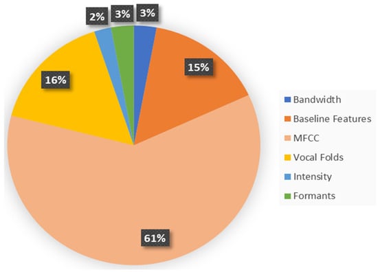
Figure 2.
The distribution of the voice features in Feature Vector I.
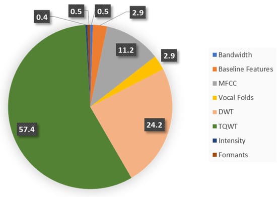
Figure 3.
The distribution of voice features in Feature Vector II.
4.1. Feature Vector I
The Jitters, Shimmers, harmonicity, recurrence period density entropy, detrended fluctuation analysis, and pitch period entropies belong to the group of baseline features. They are defined as follows:
4.1.1. Jitters
Jitters reflect the variation in successive periods of voice signals. These are determined based on the timing of the fundamental period of the glottal pulses. Following the detection of the onset time for the glottal pulses, the Jitters are determined using a set of formulas [26]. The formulated Jitters considered in this work are Jitter (local), Jitter (local absolute), Jitter (rap), Jitter (ppq5), and Jitter (ddp).
4.1.2. Shimmers
Unlike Jitters, Shimmers focuses on the peak values of a signal. They are formulated based on the onset time of the glottal pulses of a voice signal’s and the signal’s respective magnitude. The investigated Shimmer parameters are: Shimmer (local), Shimmer (local, dB), Shimmer (apq3), Shimmer (apq5), Shimmer (apq11), and Shimmer (ddp) [26].
4.1.3. Harmonicity
Harmonicity represents the degree of periodicity of an acoustic signal. This work considered three harmonicity parameters: mean autocorrelation, noise-to-harmonics ratio, and harmonics-to-noise ratio (HNR).
4.1.4. Recurrence Period Density Entropy (RPDE)
The RPDE is used to determine the periodicity level of a voice signal [27]. All pathological voice signals reside between two extremes: perfect periodicity and complete randomness. The RPDE is measured from the recurrence time probability density function and is used to discriminate voice disorders from healthy voices. The ranking is measured from the recurrence time probability density function using a sliding scale between a purely periodic and a random signal. One informative measure of any probability density function is entropy, which measures the average uncertainty of the discrete-valued density function. , i = 1, 2…M by
where is the number of samples.
For a purely periodic signal, the RPDE is defined as
where is the maximum recurrence time. On the other hand, for a purely stochastic signal, the RPDE is defined by
Hence, the RPDE of a disordered voice signal will be in the range between and .
4.1.5. Detrended Fluctuation Analysis (DFA)
In stochastic processes, detrended fluctuation analysis (DFA) is a method used to determine the statistical self-affinity of a signal [27]. It helps analyze time-series data that are considered long-memory processes. The DFA is computed using the following steps: First, the signal is integrated to produce another stochastic signal by
where is the time-series data, n = 1,2,3,….N (N is the number of samples in the dataset). Then, is divided into a window of samples. A least-squares straight-line local trend is calculated by analytically minimizing the squared error, over the slope and intercept parameters and by
Next, the root-mean-square deviation from the trend (i.e., the fluctuation) is calculated over every window at every time scale by
This process is repeated over the whole signal at various window sizes .
4.1.6. Pitch Period Entropy (PPE)
PPE is another essential voice feature. First, the pitch sequence is extracted from the voice samples and is converted to the logarithmic semitone scale, , where is the semitone pitch at a time . Then, linear temporal correlations in this semitone sequence are removed with a standard linear whitening filter to produce the relative semitone variation sequence . Subsequently, a discrete probability distribution of occurrence for relative semitone variations, is determined. Finally, the entropy is calculated [27].
4.1.7. Intensity Features
The minimum, maximum, and mean intensities of the voice signal were used in this investigation. These parameters are defined as follows:
- Minimum Intensity: This is the lowest sound pressure level (SPL) that a voice can produce. This is often close to the threshold of hearing for an individual.
- Maximum Intensity: This is the highest SPL that a voice can produce. The physical capabilities of the vocal folds and respiratory system limit it.
- Mean Intensity: This is the average SPL over a period or a sample of voice signals. This represents the typical loudness level of a person’s voice.
4.1.8. Formants
A formant usually refers to the entire spectral contribution of a resonance [28,29]. The peaks of the spectrum for the vocal tract response correspond to its formants (approximately). In this work, the first four formant frequencies () have been included to form the feature vector.
4.1.9. Vocal Fold Parameters
The vocal fold vibration pattern is an essential phenomenon in speech production [30,31,32]. This is the result of the interaction between the vocal folds and airflow. Vibration has been the subject of much research for the detection of voice disorders. This investigation includes the following vocal fold parameters: glottal quotient (GQ), glottal-to-noise excitation (GNE) ratios, vocal fold excitation ratios (VFERs), and intrinsic mode functions (IMFs).
4.1.10. The MFCC
The MFCCs are determined using the following procedure [33,34]. The voice sample is first segmented with an analysis window and the short-time Fourier transform (STFT), is computed by
where with being the discrete Fourier transform (DFT) length. The magnitude of is then weighted by a series of filter frequency responses whose center frequencies and bandwidths match with the auditory critical band filters called mel-scale filters. The next step is to compute the energy in the STFT weighted by each mel-scale filter frequency response. The energies for each speech frame at the time and for the l-th mel-scale filter are given by
where is the frequency response of the th mel-scale filter, and Ul are the lower and upper-frequency indices over which each filter is non-zero, while is defined as
Finally, the cepstrum, associated with, is computed for the speech frame at time n by
where is the number of filters. In this work, 13 MFCCs and their delta and delta-delta coefficients were measured by processing voice signals using a Mel filter bank. The delta coefficients were obtained by computing the difference between two MFCCs at two different windows. The delta-delta coefficients were computed by replacing the mel coefficients with delta coefficients.
4.2. Feature Vector II
The above-mentioned Feature Vector I is extended further by including wavelet-based features. In this investigation, two wavelet features were included: discrete wavelet transform (DWT)-based features and tunable Q wavelet transform (TQWT)-based features. DWT and TQWT are more suitable for measuring the local frequency content in non-stationary signals like voice signals, than the traditional Fourier transform. Another significant advantage of the wavelet over the conventional Fourier transform is that it can provide accurate information about the fast fluctuations of signals in the time domain. Hence, it is another useful and important feature that can help detect PD voice samples. We first discuss the continuous wavelet transform and then extend the discussion to the DWT and TQWT. The continuous wavelet transform (CWT) of a signal is defined as
where is the primary wavelet function, is the time shift, and is the scaling factor. Conceptually, is a measure of “similarity” between and at different scales and time shifts. Based on the definition of convolutional integration, can be expressed as
Considering computational efficiency, this work considers DWT instead of CWT. We begin by coding the signal using a wavelet expansion as follows:
By applying and continuing to apply (13), can be coded at any level we wish. In this work, was coded to 10 levels. By recursively applying (13) until , we can obtain signal expansion using all the mother wavelets plus one scaling function at scale , that is
All and all are called the wavelet coefficients. They are essentially the weights for the scaling and wavelet functions (mother wavelets). The DWT computes the wavelet coefficients. Based on wavelet theory, we can perform DWT using the following analysis equations:
where are the low-pass wavelet filter coefficient and are the high-pass filter coefficient that can be determined by
These low-pass and high-pass filters are called quadrature mirror filters (QMF). The expression presented in (14) can be simplified further to compute the and in a more efficient way [35,36].
In this investigation, the “Haar” wavelet function was used as the mother wavelet. Although several wavelet families are available, the Haar wavelet function was adopted in this investigation for the following reasons: (a) Haar wavelets are the simplest form of wavelets and are easy to compute compared to other wavelets; (b) they are beneficial in real-time processing scenarios where speed is a concern; and (c) these wavelets are particularly effective for detecting discontinuities in the voice samples of patients with Parkinson’s disease [37,38].
The expansion coefficients are computed using recursive filtering and downsampling (i.e., filter bank). The first stage of the filter bank divides the spectrum into low-pass and high-pass bands. The second stage divides the lower half into two quarters, and so on. Each filter maintains a “constant-Q”. That means , where is the filter bandwidth and is the center frequency. The wavelet expansion coefficients were extracted by applying a 10-level DWT to the voice samples. After decomposition, the energy, Shannon’s and log energy entropies, and Teager−Kaiser energy were computed based on the DWT.
In the basic DWT, the Q-factor is fixed. However, the Q-factor of the wavelet must be adaptable to input signals. Oscillatory signals, like speech, require a high Q-factor. In contrast, a signal with no or low oscillatory behavior requires a low Q-factor. To overcome this limitation, which is inherent to most wavelet transforms, the TQWT was introduced. Similar to the traditional wavelet transform, the TQWT is computed using iterative filtering. The lower-band signal is processed using a low-pass scaling filter, and the higher-band signal is processed using a high-pass scaling filter. Using a low-pass scaling filter, the low-frequency content of the speech signal is preserved and vice versa. For low-pass scaling, the scaling parameter is used. If the sampling frequency of the input signal is, , then the low-pass filtering changes this frequency to . When, , the Fourier transform of the output signal is given by
When, , the output is given by
For high-pass scaling, the scaling factor is used, and the output signal frequency is scaled by this factor . For the Fourier transform of the filtered output signal is defined by
For , the Fourier transform of the output signal is given by
By using the scaling parameters, and more parameters, including Q-factor (, oversampling rate (), center frequency (), and bandwidth ( are defined as follows.
where is the level of the wavelet transform. In this work, and have been used to generate the data. In addition to the TQWT coefficients, the energy and entropy measures of each level are also included to form a significant part of the feature matrix used in this work.
5. Methods
The design of the machine learning algorithms, namely kNN and SVM, is conducted using MATLAB 2020. The system model is shown in Figure 4. The proposed algorithm applies different signal-processing techniques to extract clinically useful features from voice recordings of patients with PD and healthy participants. Then, a feature vector is formed. This is a data reduction technique. PCA is applied to minimize data redundancy. Finally, SVM and kNN are applied to classify the samples as PD or healthy.
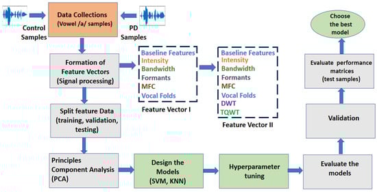
Figure 4.
The system model employs data reduction techniques (PCA) and classification algorithms (SVM and kNN) to identify patients with PD from healthy individuals with predominant voiced (‘/a/’) features.
5.1. PCA
High-dimensional data are difficult to generalize and may lead to overfitting of the classification performance of machine learning models. PCA linearly transforms feature vectors to remove redundancy in dimensions, thus generating a new set of principal components. PCA is performed in several steps, as mentioned in [39]. To reduce the dimension of the feature matrix, PCA with 0.95 variances is used in this work.
5.2. SVM
SVM is one of the most popular machine learning algorithms. SVM applies a statistical concept (i.e., support vector) to classify data. Objects in a classification problem are represented by vectors from some vector space . Although SVMs can be used in arbitrary vector spaces supplied with the inner product or kernel function, in most practical applications, vector space is simply the -dimensional real coordinate space defined by . In this space, vector is a set of real numbers being the components of the vector (i.e., ). A sample of objects with known class labels is called a training set and is written as where ∈ {−1, 1} is the class label of the vector , and is the size of the training set. A classification algorithm (or simply classifier) is represented by a decision function such that if the classifier assigns to the first class and if the classifier assigns to the second class. In the coordinate space , the equations and define a dimensional set of vectors called a hyperplane. That is for a given non-zero vector and a scaler , the set of all vectors satisfying form a hyperplane. Let us denote the hyperplane by . Vector is called the normal vector of the hyperplane, and number is called the intercept of the hyperplane. We can say that a hyperplane separates two classes (sets) of vectors and to satisfy the conditions , and , . Two classes are called linearly separable if at least one hyperplane separates them. If hyperplane separates classes and according to the above-mentioned conditions, then the decision function will be defined as , where the signum function is defined as when and when . The parameters and of the SVM hyperplane can be found as a solution to the following optimization problems. subject to the conditions , and , . However, it is difficult to identify a linear separation plane in the dimensional feature space formed by the investigated feature matrix mentioned above. To solve this problem, this work applies linear, quadratic, cubic, and Gaussian kernels for the classification tasks performed by the SVM.
5.3. kNN
kNN achieves consistently high performance without a priori assumptions regarding the distribution of the training data. Similar to the SVM, the data consists of a training set and a test set for the kNN classification. The training set is a set of feature vectors and their class labels; and a learning algorithm is used to train the kNN classifier using the training set. An intuitive way to decide how to classify an unlabeled test item is to look at the training data points nearby and classify them according to the classes of those nearby labeled data points. This intuition is formalized in a classification approach called the k-nearest neighbor (kNN) classification. The kNN approach looks at the points in the training set that is closest to the test point; the test point is then classified according to the class to which the majority of the -nearest neighbors belong. A new sample is classified by calculating the distance to the nearest training case. If the Euclidean distance is used as the distance metric, this distance can be defined by
Finally, the data is assigned to a class with the largest probability defined by
where feature matrix, class label, set of k-nearest observations, evaluates if an observation in is a member of the class and otherwise.
The kNN algorithm determines the class of an unspecified point by counting the majority class votes from the kNN training points. The value of is an important factor for the regularization of the kNN. It is common to select small (i.e., 1) and odd to break ties (typically 3, 5, 7, etc.). Larger values help reduce the effects of noisy points within the training data set, and the choice of is often determined through cross-validation [40].
6. Results
The statistical performance of the proposed models was evaluated using the following parameters: (a) true positive (TP), (b) true negative (TN), (c) false negative (FN), and (d) false positive (FP).
Five-fold cross-validation schemes were adopted to train the classifiers. Since the main goal of this investigation is to consider the effects of the wavelet features in PD detection, two cases were considered in the simulations: (a) voice features excluding wavelet transform-based features (i.e., Feature Vector I) and (b) voice features including wavelet transform-based features (i.e., Feature Vector II).
6.1. Results with Feature Vector I
The results provided by the SVM and kNN are presented in Table 1. The SVM provided the best results when the Gaussian kernel function was used with a scale of 10.1402. In contrast, kNN provided the best results with fine kNN (k = 1) and Euclidean distance metric. The TP, TN, FP, and FN values were 537, 113, 79, and 27 for the SVM, respectively, whereas these values were 534, 141, 51, and 30 for the kNN.

Table 1.
The Simulation Results of the SVM and kNN Algorithms with Feature Vector 1.
The performances of these two machine learning algorithms were investigated and compared in terms of accuracy, precision, sensitivity, F1-score, NPV, specificity, FNR, FDR, G-mean, Matthews correlation coefficient (MCC), and AUC, as listed in Table 2. An accuracy of 89.29% was achieved with the fine kNN, as listed. The data presented in Table 2 also shows that the precision, sensitivity, F1-score, NPV, specificity, FNR, FDR, G-mean, MCC, and AUC for the kNN are 91.28%, 94.68%, 92.95%, 82.46%, 73.44%, 8.72%, 17.54%, 83.39%, 70.87%, and 0.84. In contrast, an accuracy of 85.98% was achieved with the SVM. The precision, sensitivity, F1-score, NPV, specificity, FNR, FDR, G-mean, MCC, and AUC for the SVM were 87.18%, 95.21%, 91.02%, 80.71%, 58.85%, 12.82%, 19.29%, 74.86%, 60.59% and 0.91, respectively. The comparison parameters of the two machine learning algorithms are presented in Figure 5. This figure shows that there were no significant differences in the performance parameters of these two algorithms, except for specificity and MCC. The higher specificity of kNN indicates that it correctly identified most of the healthy samples compared to SVM, as listed in Table 2. The higher MCC for kNN also indicates that it provided a higher correlation between the predicted and actual binary outcomes than SVM. Additional performance parameters, including misclassification cost, prediction rate, and training time, are listed in Table 3. This table also demonstrates the superiority of kNN over SVM. For example, the training period of kNN (i.e., 44.01 s) was less than that of SVM (i.e., 201.21 s). Even the misclassification cost is 81 for the kNN, which is much lower than that of the SVM (i.e., 106).
Table 2.
The performance comparison of SVM and kNN (with Feature Vector I).
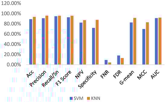
Figure 5.
The performance comparison of SVM and kNN (with Feature Vector I).
Table 3.
The comparison of the other performance indicators (with Feature Vector I).
6.2. The Results with Feature Vector II
Further simulations were conducted using the same set of PD and control voice samples. However, Feature Vector II includes the DWT and TQWT transform-based features, as mentioned above. The same machine learning algorithms (i.e., SVM and kNN) were considered classifiers. The performances of the SVM and kNN in terms of TP, TN, FP, and FN are listed in Table 4. These values were 534, 138, 54, and 30 for the SVM and 539, 168, 24, and 25 for the kNN, respectively. This table shows that kNN outperforms SVM in detecting both the PD and control subjects. The performances of these two machine learning algorithms in terms of accuracy, precision, sensitivity, F1-score, NPV, specificity, FNR, FDR, G-mean, MCC, and AUC are listed in Table 5. An accuracy of 93.52% was achieved with kNN, which is 4.63% higher than the accuracy achieved with SVM, as listed in Table 5. The precision, sensitivity, F1-score, NPV, specificity, FNR, FDR, G-mean, MCC, and AUC for kNN were 95.74%, 95.57%, 95.65%, 87.05%, 87.50%, 4.26%, 12.95%, 91.44%, 82.93%, and 0.92, respectively. In contrast, the precision, sensitivity, F1-score, NPV, specificity, FNR, FDR, G-mean, MCC, and AUC for the SVM are 90.82%, 94.68%, 92.71%, 82.14%, 71.88%, 9.18%, 17.86%, 82.49%, 69.68%, and 0.91, respectively.
Table 4.
The simulation results of the SVM and kNN algorithms with Feature Vector II.
Table 5.
The performance comparison of SVM and kNN with Feature Vector II.
A comparison of these performances is shown in Figure 6, which shows that the specificity, G-mean, and MCC for the kNN are significantly higher than those for the SVM. These improvements in the performance of the investigated machine learning algorithms are higher than those listed in Table 2. Other performance indicators, including the misclassification rate, training time, and prediction time, are listed in Table 6. This table also demonstrates that kNN needs less time to be trained than SVM. In addition, the misclassification rate was lower for kNN. However, the prediction speed is lower for kNN. Comparing the data presented in Table 6 and Table 3, we can conclude that the wavelet-based features help the investigated learning algorithms reduce the misclassification rates. However, the wavelet-based features reduce the prediction speed, as demonstrated in Table 3 and Table 6. These features also increase the training time required.
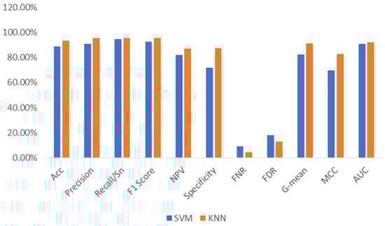
Figure 6.
The performance comparison of SVM and kNN (with Feature Vector II).
Table 6.
The comparison of other performance indicators.
Based on the simulation results presented in this section, we can conclude that wavelet-based features can play an important role in PD detection using voice features and machine learning algorithms. We can also conclude that the kNN algorithm is more suitable than SVM for PD detection. kNN requires less time to train than SVM. In addition, the kNN provides fewer misclassification errors. The confusion matrix, minimum classification error, and AUC for the kNN model are plotted in Figure 7, Figure 8, and Figure 9, respectively. The confusion matrix shown in Figure 7 demonstrates that kNN provides an unbiased classification. The kNN model successfully detected 539 PD patients out of 564 samples. It failed to detect pathology in only 25 instances. The kNN also performed equally well in detecting the control subjects. Of the 192 control samples, kNN successfully detected 168 samples and missed 24 samples. The minimum misclassification error curve presented in Figure 8 shows the excellent performance of the kNN model. The figure demonstrates that kNN provides the minimum misclassification error within a few iterations (around 22 iterations). The AUC curve is shown in Figure 9. This curve demonstrates that an AUC of 0.92 was achieved with kNN when the wavelet features were included in the feature vector.
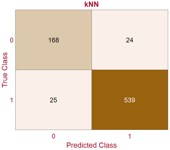
Figure 7.
The confusion matrix of the kNN with Feature Vector II (‘1’ indicates Parkinson’s disease and ‘0’ indicates control samples).
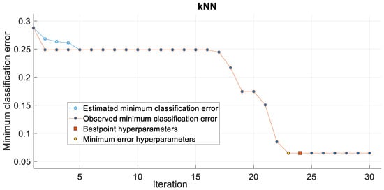
Figure 8.
The classification error with kNN.
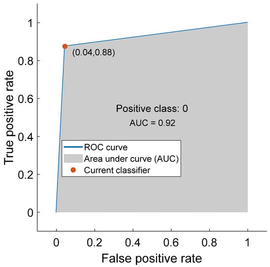
Figure 9.
The area under the curve (AUC) for kNN (with Feature Vector II).
The performance of the proposed model was compared with that of other existing related works mentioned in Section 2. The performance comparison is listed in Table 7. The proposed model outperforms the similar PD detection algorithms presented in [13,14,17,18,21], as listed in the table. The performance of the algorithms presented in [12,20,22] is almost similar to that of the proposed model. However, the algorithms presented in [16,19,23,24] outperform the proposed model, as demonstrated in Table 7.
Table 7.
The Comparative Analysis.
7. Conclusions
To date, Parkinson’s disease is considered a chronic disease, and there is no treatment to deter its progression. Early diagnosis can facilitate holistic Parkinson’s disease management through medications, physical therapy, and maintaining a supportive environment for the patient, healthcare professionals, and the patient’s relatives. As mentioned before, atypical brain activity caused by PD leads to impaired movement, tremors, slowed movement, rigid muscles, and unconscious motion. Notably, PD also causes changes in speech. Hence, speech signals can be a good biomarker for early PD symptoms, as demonstrated in this paper. We have shown that a judicious choice of voice features and machine learning models can facilitate the early detection of PD, which consequently leads to assistive living for patients with PD during the progression level of this disease.
This paper shows that the voice samples contain useful information that can detect PD at an early stage. A wide variety of multi-domain acoustic features were extracted from voice samples and applied to optimize two competing machine learning algorithms, the kNN and SVM algorithms, for classification. These two machine learning algorithms were employed because of ongoing debates regarding their performance in classification tasks. The results demonstrated that the investigated voice features and machine learning algorithms had high discriminative power for identifying PDs with excellent performance. Even the problem of imbalanced data samples for diseased and healthy classes (i.e., 92 healthy and 564 PDs) is overcome by selecting robust voice features and designing a proper machine learning algorithm.
The simulation results also concluded that wavelet features are important for detecting neurodegenerative diseases like PD. It was also shown that including the wavelet features can significantly improve the performance of the machine learning algorithms. This paper also concludes that the kNN outperforms the SVM algorithm for the investigated voice features despite the inclusion and exclusion of the wavelet features. However, wavelet features can further enhance the performance of these machine learning algorithms.
This paper focused only on the detection of PDs. The detection of the progression level of PDs needs to be considered in the future. The contribution of the feature matrix in different domains and gender considerations for classification performance is left as future work. This work employed only two popular machine learning models. Investigating other machine learning and deep learning algorithms has also been left as future work.
Author Contributions
Conceptualization, analysis, methodology, software, data curation, validation, reviews, manuscript writing, R.I.; review and editing, M.T. All authors have read and agreed to the published version of the manuscript.
Funding
This research received no external funding.
Institutional Review Board Statement
Not applicable.
Informed Consent Statement
Not applicable.
Data Availability Statement
Publicly available datasets were analyzed in this study. These data can be found here: https://archive.ics.uci.edu/dataset/470/parkinson+s+disease+classification accessed on 15 March 2025.
Conflicts of Interest
The authors declare no conflicts of interest.
References
- American Association of Neurosurgeons. Parkinson’s Disease. Available online: https://www.aans.org/patients/conditions-treatments/parkinsons-disease/ (accessed on 8 January 2025).
- World Health Organization. Parkinson’s Disease: Key Facts. Available online: https://www.who.int/news-room/fact-sheets/detail/parkinson-disease (accessed on 8 January 2025).
- Parkinson, J. An Essay on Shaking Palsy. J. Neuropsychiatry Clin. Neurosci. 2002, 14, 223–236. [Google Scholar] [CrossRef] [PubMed]
- John Hopkins Medicine. Parkinson’s Symptoms. Available online: https://www.hopkinsmedicine.org/health/conditions-and-diseases/parkinsons-disease (accessed on 8 January 2025).
- Braak, H.; Ghebremedhin, E.; Rüb, U.; Bratzke, H.; Tredici, K.D. Stages in the development of Parkinson’s disease-related pathology. Cell Tissue Res. 2004, 318, 121–134. [Google Scholar] [CrossRef] [PubMed]
- Islam, R.; Abdel-Raheem, E.; Tarique, M. Cochleagram to Recognize Dysphonia: Auditory Perceptual Analysis for Health Informatics. IEEE Access 2024, 12, 59198–59210. [Google Scholar] [CrossRef]
- Sakar, B.E.; Isenkul, M.E.; Sakar, C.O.; Sertbas, A.; Gurgen, F.; Delil, S.; Apaydin, H.; Kursun, O. Collection and analysis of a Parkinson speech dataset with multiple types of sound recordings. IEEE J. Biomed. Health Inform. 2013, 19, 828–834. [Google Scholar] [CrossRef]
- Logemann, J.A.; Fisher, H.B.; Boshes, B.; Blonsky, E.R. Frequency and Occurrence of Vocal Tract Dysfunction in the Speech of a large samples of Parkinson’s Patients. J. Speech Hear. Disord. 1978, 43, 47–57. [Google Scholar] [CrossRef]
- Ho, K.; Iansek, R.; Marigliani, C.; Bradshaw, J.L.; Gates, S. Speech impairment in a large sample of patients with Parkinson’s disease. Behav. Neurol. 1999, 11, 131–137. [Google Scholar] [CrossRef] [PubMed]
- Islam, R.; Tarique, M.; Abdel-Raheem, E. A survey on signal processing based pathological voice detection techniques. IEEE Access 2020, 8, 66749–66776. [Google Scholar] [CrossRef]
- Islam, R.; Abdel-Raheem, E.; Tarique, M. A study of using cough sounds and deep neural networks for the early detection of COVID-19. Biomed. Eng. Adv. 2022, 3, 100025. [Google Scholar] [CrossRef] [PubMed]
- Karimi-Rouzbahani, H.; Daliri, M. Diagnosis of Parkinson’s disease in Humans using Voice Signals. Basic Clin. Neurosci. 2011, 2, 12–20. [Google Scholar]
- Little, M.A.; McSharry, P.E.; Hunter, E.J.; Spielman, J.; Ramig, L.O. Suitability of Dysphonia Measurements for Telemonitoring of Parkinson’s Disease. IEEE Trans. Biomed. Eng. 2009, 56, 1015–1022. [Google Scholar] [CrossRef]
- Islam, R.; Abdel-Raheem, E.; Tarique, M. Voiced Features and Artificial Neural Network to Diagnose Parkinson’s Disease Patients. In Proceedings of the International Conference on Electrical and Computing Technologies and Applications, Ras Al Khaimah, United Arab Emirates, 23–25 November 2022; pp. 132–136. [Google Scholar] [CrossRef]
- Tsanas, A.; Little, M.A.; McSharry, P.E.; Ramig, L.O. Accurate Telemonitoring of Parkinson’s Disease Progression by Noninvasive Speech Tests. IEEE Trans. Biomed. Eng. 2010, 57, 884–893. [Google Scholar] [CrossRef]
- Solana-Lavalle, G.; Rosa-Romero, R. Analysis of voice as an assisting tool for detection of Parkinson’s disease and its subsequent clinical interpretation. Biomed. Signal Process. Control. 2021, 66, 102415. [Google Scholar] [CrossRef]
- Sakar, C.O.; Serbes, G.; Gunduz, A.; Tunc, H.C.; Nizam, H.; Sakar, B.E.; Tutuncu, M.; Aydin, T.; Isenkul, M.E.; Apaydin, H. A comparative analysis of speech signal processing algorithms for Parkinson’s disease classification and the use of tunable Q-factor wavelet transform. Appl. Soft Comput. 2019, 74, 255–263. [Google Scholar] [CrossRef]
- Das, R. A comparison of multiple classifications methods for diagnosis of Parkinson’s disease. Expert Syst. Appl. 2010, 37, 1568–1572. [Google Scholar] [CrossRef]
- Shirvan, R.A.; Tahami, E. Voice Analysis for Detecting Parkinson’s Disease using Genetic Algorithm and KNN Classification methods. In Proceedings of the 18th Conference on Biomedical Engineering, Tehran, Iran, 14–16 December 2011; pp. 278–284. [Google Scholar] [CrossRef]
- Senturk, Z.K. Early diagnosis of Parkinson’s disease using machine learning algorithms. Med. Hypothesis 2020, 138, 109603. [Google Scholar] [CrossRef]
- Gil, D.; Johnson, B.M. Diagnosing Parkinson’s by using Artificial Neural Networks and Support Vector Machine. Glob. J. Comput. Sci. Technol. 2009, 9, 63–71. [Google Scholar]
- Anisha, D.; Arulanand, N. Early Detection of Parkinson’s disease (PD) using Ensemble Classifiers. In Proceedings of the International Conference on Innovative Trends in Information Technology, Kottayam, India, 13–14 February 2020; pp. 1–6. [Google Scholar] [CrossRef]
- Nissar, D.R.; Rizvi, S.M.; Mir, A.N. Voice Based Detection of Parkinson’s Disease through Ensemble Machine Learning Approach: A Performance Study. EAI Endorsed Trans. Pervasive Health Technol. 2019, 5, e2. [Google Scholar] [CrossRef]
- Salama, A.; Mostafa, A.M.; Mazin, A.M.; Raed, I.H.; Arunkumar, N.; Ghani, M.K.A.; Jaber, M.M.; Khaleefah, S.H. Examining multiple feature evaluation and classification methods for improving the diagnosis of Parkinson’s Disease. Cogn. Syst. Res. 2019, 54, 90–99. [Google Scholar] [CrossRef]
- Parkinson’s Data. Available online: https://archive.ics.uci.edu/ml/datasets/Parkinsons (accessed on 8 January 2025).
- Islam, R.; Tarique, M. Classifier Based Early Detection of Pathological Voice. In Proceedings of the IEEE International Symposium on Signal Processing and Information Technology (ISSPIT), Ajman, United Arab Emirates, 10–12 December 2019; pp. 1–6. [Google Scholar] [CrossRef]
- Little, M.A.; McSharry, P.E.; Roberts, S.J.; Costello, D.A.E.; Moroz, I.M. Exploiting Nonlinear Recurrence and Fractal Scaling Properties for Voice Disorder Detection. BioMed. Eng. Online 2007, 6, 23. [Google Scholar] [CrossRef]
- Rabiner, L.; Schafer, R. Algorithms for Estimating Speech Parameter. In Theory and Application of Digital Speech Processing, 1st ed.; Pearson: London, UK, 2011; pp. 649–659. [Google Scholar]
- Taib, D.; Tarique, M.; Islam, R. Voice Feature Analysis for Early Detection of Voice Disability in Children. In Proceedings of the 2018 IEEE International Symposium on Signal Processing and Information Technology (ISSPIT), Louisville, KY, USA, 6–8 December 2018; pp. 12–17. [Google Scholar] [CrossRef]
- Yokota, K.; Ishikawa, S.; Takezaki, K.; Koba, Y.; Kijimoto, S. Numerical analysis and physical consideration of vocal fold vibration by modal analysis. J. Sound Vib. 2021, 514, 116442. [Google Scholar] [CrossRef]
- Islam, R.; Abdel-Raheem, E.; Tarique, M. Deep Learning Based Pathological Voice Detection Algorithm Using Speech and Electroglottographic (EGG) Signals. In Proceedings of the International Conference on Electrical and Computing Technologies and Applications, Ras Al Khaimah, United Arab Emirates, 23–25 November 2022. [Google Scholar] [CrossRef]
- Islam, R.; Abdel-Raheem, E.; Tarique, M. Voice pathology detection using convolutional neural networks with electroglottographic (EGG) and speech signals. Comput. Methods Programs Biomed. Update 2022, 2, 100074. [Google Scholar] [CrossRef]
- Quateri, T.E. Production and Classification of Speech Sounds. In Discrete-Time Speech Signal Processing: Principles and Practices; Prentice Hall: Upper Saddle River, NJ, USA, 2001; pp. 72–76. [Google Scholar]
- Islam, R.; Tarique, M. Phonation Attributes and Artificial Intelligence (AI) to Delineate the Progression of Amyotrophic Lateral Sclerosis (ALS): A Neurodegenerative Disorder. In Proceedings of the International Conference on Computer Engineering, Network, and Intelligent Multimedia (CENIM), Surabaya, Indonesia, 19 November 2024; pp. 1–6. [Google Scholar] [CrossRef]
- Cortes, C.; Vapnik, V. Support-Vector Networks. Mach. Learn. 1995, 20, 273–297. [Google Scholar] [CrossRef]
- Devnath, L.; Nath, S.K.D.; Das, A.K.; Islam, M.R. Selection of Wavelet and Thresholding Rule for Denoising the ECG Signals. Ann. Pure Appl. Math. 2015, 10, 65–73. [Google Scholar]
- Tan, L.; Jiang, J. Subband and Wavelet-Based Coding. In Digital Signal Processing, 2nd ed.; Academic Press: Cambridge, MA, USA, 2013; pp. 655–658. [Google Scholar]
- Mondal, M.K.; Devnath, L.; Mazumder, M.; Islam, M.R. Comparison of Wavelets for Medical Image Compression Using MATLAB. Int. J. Innov. Appl. Stud. 2016, 18, 1023–1031. [Google Scholar]
- Islam, R.; Tarique, M. Blind Source Separation of Fetal ECG Using Fast Independent Component Analysis and Principle Component Analysis. Int. J. Sci. Technol. Res. 2020, 9, 80–95. [Google Scholar]
- Islam, R.; Abdel-Raheem, E.; Tarique, M. Parkinson’s Disease Detection Using Voice Features and Machine Learning Algorithms. In Proceedings of the International Conference on Microelectronics (ICM), Abu Dhabi, United Arab Emirates, 17–20 December 2023; pp. 96–100. [Google Scholar] [CrossRef]
Disclaimer/Publisher’s Note: The statements, opinions and data contained in all publications are solely those of the individual author(s) and contributor(s) and not of MDPI and/or the editor(s). MDPI and/or the editor(s) disclaim responsibility for any injury to people or property resulting from any ideas, methods, instructions or products referred to in the content. |
© 2025 by the authors. Licensee MDPI, Basel, Switzerland. This article is an open access article distributed under the terms and conditions of the Creative Commons Attribution (CC BY) license (https://creativecommons.org/licenses/by/4.0/).