Article

Weighted Trajectory Analysis and Application to Clinical Outcome Assessment

1
Faculty of Medicine and Dentistry, University of Alberta, Edmonton, AB T6G 2R7, Canada
2
Department of Mathematics and Statistics, York University, Toronto, ON M3J 1P3, Canada
3
Division of Medical Oncology, Cross Cancer Institute, University of Alberta, 11560 University Ave NW, Edmonton, AB T6G 1Z2, Canada
*
Author to whom correspondence should be addressed.
BioMedInformatics 2023, 3(4), 829-852; https://doi.org/10.3390/biomedinformatics3040052
Submission received: 11 August 2023 / Revised: 1 September 2023 / Accepted: 25 September 2023 / Published: 7 October 2023
(This article belongs to the Special Issue Feature Papers in Medical Statistics and Data Science Section)

Abstract

:
The Kaplan–Meier (KM) estimator is widely used in medical research to estimate the survival function from lifetime data. KM estimation is a powerful tool to evaluate clinical trials due to simple computational requirements, its use of a logrank hypothesis test, and the ability to censor patients. However, KM estimation has several constraints and fails to generalize to ordinal variables of clinical interest, such as toxicity and ECOG performance. We devised weighted trajectory analysis (WTA) to combine the advantages of KM estimation with the ability to visualize and compare treatment groups for ordinal variables and fluctuating outcomes. To assess statistical significance, we developed a new hypothesis test analogous to the logrank test. We demonstrated the functionality of WTA through 1000-fold clinical trial simulations of unique stochastic models of chemotherapy toxicity and schizophrenia disease course. With increments in sample size and hazard ratio, we compared the performance of WTA to KM estimation and the generalized estimating equation (GEE). WTA generally required half the sample size to achieve comparable power to KM estimation; advantages over the GEE included its robust nonparametric approach and summary plot. We also applied WTA to real clinical data: the toxicity outcomes of melanoma patients receiving immunotherapy and the disease progression of patients with metastatic breast cancer receiving ramucirumab. The application of WTA demonstrated that using traditional methods such as KM estimation can lead to both type I and II errors by failing to model illness trajectory. This article outlines a novel method for clinical outcome assessment that extends the advantages of Kaplan–Meier estimates to ordinal outcome variables.

1. Introduction

The Kaplan–Meier (KM) estimator [1], also referred to as the product-limit estimator, is widely used in medical research to estimate the survival function from lifetime data. KM estimation is a nonparametric approach for time-to-event data, which are often not normally distributed. To generate the KM estimates, the time-to-event and the status of each subject at the last observed timepoint are needed [2]. The event of interest may be death from any cause when we are determining overall survival and death due to a specific cause for cause-specific survival. KM estimates are frequently used in oncology and other medical disciplines. KM estimation is used to compare two or more treatment arms in clinical trials using the logrank test [3]. Patients that exit the trial without having experienced the event of interest at the last follow up are censored and omitted from further estimates.
The relatively simple computational requirements for KM estimation provide a powerful method to estimate time-to-event data. However, the advantages of KM estimation in clinical research cannot be extended to important ordinal outcomes, such as toxicity grade and Eastern Cooperative Oncology Group (ECOG) performance status [4]. Ordinal outcome variables are ubiquitous in medicine in the measurement of patient health status over time, but no statistical methods exist that combine censoring, graphical comparison of trajectories, and hypothesis testing for these variables. Often, ordinal clinical outcomes are collapsed to binary definitions to facilitate the use of KM estimation; this causes information loss, introduces an arbitrary cutpoint, and may lead to inaccurate conclusions. New methods are required to map the trajectory of ordinal outcomes and compare treatment arms in clinical trials.
The KM method has three conditions that limit its generalizability to other variables of interest in clinical research:
  • Binary Condition
    The event must be binary in nature or coded into binary form (0 for non-occurrence, 1 for occurrence). It is not possible to capture grades or stages of severity. For example, death is naturally binary (0 for alive, 1 for dead), but an outcome variable such as toxicity (measured in grades from zero to four) must be coded into binary form by setting a threshold for event occurrence, such as arbitrarily defining an event as any toxicity exceeding grade two;
  • Descent Condition
    Event occurrence always produces a drop in the KM curve (a consequence of plotting probability). It is not possible to track the trajectory of conditions that can both improve and worsen over time. For example, patients experiencing rising toxicity due to chemotherapy require additional interventions to tolerate therapy. The interventions may initially improve symptoms and reduce toxicity grade but fail to sustain benefits in subsequent treatment cycles. For a KM estimate following the above example, this complex trajectory would be simplified to an event occurrence the first time toxicity increases beyond grade two;
  • Finality Condition
    Once a patient experiences the event of interest, they are omitted from any subsequent analysis.
Weighted trajectory analysis (WTA) is a method that combines the simplicity and practicality of KM estimation with the ability to compare treatment groups for ordinal variables and bidirectional outcomes. Trajectories are presented using plots that track health status for treatment arms over time. WTA permits the censoring of patients that exit the study. To determine statistical significance, we developed a “weighted” logrank test.
In Section 2, we describe the methodology and theory of KM estimation and WTA, along with their respective hypothesis tests, and provide a computational approach to WTA that is robust with smaller datasets. We also outline GEE longitudinal analysis prior to its use as an additional comparator against WTA in subsequent simulation studies. In Section 3 and Section 4, we describe unique simulation studies with chemotherapy toxicity grade and schizophrenia symptom stage as the variables of interest, respectively. In Section 5, we apply WTA to real clinical datasets: first, with the toxicity outcomes of melanoma patients receiving different immunotherapy protocols and, second, with tumor response outcomes of patients with metastatic breast cancer receiving an anti-angiogenic drug. Finally, we discuss the results and implications of both our simulations and real-world analyses in Section 6.

2. Methodology and Theory

2.1. Kaplan–Meier Estimator

The goal of the Kaplan–Meier (KM) estimator is to estimate a population survival curve from a sample with incomplete time-to-event observations [1]. “Survival” times need not relate to death but can refer to any event of interest, such as local recurrence or stroke. The event in this instance is a binary variable, meaning that samples have either experienced the event up to a given time point or not. The times to failure for each subject are thus characterized by two variables: (1) serial time and (2) outcome of event occurrence or censorship.
Suppose that t 0 < t 1 < t 2 < < t K are the K distinct failure times observed in the sample. We write n j and d j as the number of patients at risk and number of events at time t j , respectively, where j = 1 , 2 , K . Note that the patients who are lost to follow up or withdraw from the trial before experiencing the event of interest (i.e., censored samples) are taken out of the risk set at the subsequent time points.
The KM estimate at time t j , S ( t j ) ^ , is calculated as the cumulative survival probability up to and including time t j ,
S ( t k ) = j = 1 k 1 d j n j ,
where S ( t ) = 1 for t < t 1 . The Kaplan–Meier curve is plotted as a stepwise function representing the change in survival probability over time.
To compare treatment arms, multiple survival functions are plotted together, enabling the comparison of differences in survival experience between groups. Treatment options can be compared using metrics such as median survival and hazard ratios. The logrank test is used to assess if the differences are statistically significant: this test and its modification for WTA are discussed in Section 2.4 and Section 2.5, respectively.

2.2. Weighted Trajectory Analysis

Weighted trajectory analysis (WTA) is a modification of KM estimation that provides the following advantages:
  • Assesses outcomes defined by various ordinal grades (or stages) of clinical severity;
  • Permits continued analysis of participants following changes in the variable of interest;
  • Demonstrates the ability of an intervention to both prevent the exacerbation of outcomes and improve recovery, as well as the time course of these effects.
Several properties of KM curves crucial for clinical trial evaluation are incorporated within WTA. The test is nonparametric and provides the ability to censor patients that withdraw or are lost to follow up. Outcomes for various treatment arms can be assessed using a summary plot that depicts all patients in serial time. The test for significance is a modification of the logrank test described by Peto et al., which is the standard method for comparing KM survival curves [3]. The logrank test is described in Section 2.4 and the weighted logrank test follows in Section 2.5. As the analytical form of the test is a conservative estimate that operates under the normal approximation, a more computationally intensive simulated approach is outlined in Section 2.6.
In WTA, an event is a change in grade or stage or, more generally, a severity score. The severity score must be ordinal but can have an arbitrary range of severity that depends on the variable of interest (for example, I–IV for heart failure class [5]). Unlike KM estimation, an event does not omit the patient from subsequent analysis. Both increases and decreases in variables of interest are captured as events. Participants can enter trajectory analysis at any starting stage, though inferences on trial results are most powerful if treatment arms are randomized to the same median starting stage.
Redefining the event allows clinical assessment of the overall trajectory of a group of patients, mapping both deterioration and improvement in health status over time. Graphically, the staircase representing survival in the Kaplan–Meier estimator always descends. The WTA staircase can both descend and rise over time to capture the dynamics of a patient’s clinical status.
Variables of interest can include any ordinal outcome variables with a defined, finite range. Examples include ECOG performance [4] and Common Terminology Criteria for Adverse Events (CTCAE) toxicity scores [6], both with ordinal scoring that ranges from 0 to 5.
For this reason, a binary variable such as death (0, alive vs. 1, dead) is not an appropriate variable of interest. In this circumstance, the range of the ordinal variable is set to 1, and the modified significance test reduces to the standard logrank test. Conversely, ECOG performance is an appropriate variable of interest given that it is ordinal with a defined range and can both improve and worsen over time. In WTA, a higher score in the variable of interest generally represents poorer health status. Variables that follow the opposite trend can be adapted to WTA by simply reversing the polarity of the ordinal scale.
Censoring in WTA is similar to KM estimation. Patient loss to follow up and withdrawal requires censoring, but patients may experience several events prior to being censored. Censoring is represented on the plot using a Wye symbol (Biomedinformatics 03 00052 i001). The number of patients remaining within the study is tabulated below the plot at evenly spaced time intervals for each treatment arm.
Table 1 directly compares KM estimation and WTA based on core features.

2.3. Mathematical Overview of Weighted Trajectory Analysis

Weighted trajectory analysis plots the health status of treatment arms as a function of time. Time values must be discrete but can correspond to days, weeks, months, or any chosen interval. For each time value on the x-axis, there is a corresponding score on the y-axis: a weighted health status. The higher the weighted health status, the healthier the group is. This score is scaled by the initial size of the treatment arm to facilitate simple comparison of groups with unequal size.
Consider a group of n patients with toxicity grades ranging from grade zero (asymptomatic/mild toxicity) to grade five (death related to an adverse event). The weighted health status at time point j is denoted by U j , where j = 0, 1, …, z. For each treatment arm, U j has a maximum value of 1 and a minimum value of 0. Suppose we begin a trial with all patients having no disease burden at grade zero: U j = U 0 = 1. A trial with the highest possible morbidity requires all patients to experience grade five toxicity (death): at this point, U j will drop to 0.
We let g i , j represent the severity score for the ith patient at time j, i = 1, …, n. The severity score is identical to their ordinal score for the variable of interest. If the range of the ordinal variable of interest does not have 0 as one extreme end, all values must be shifted to set 0 as the starting score (the polarity may also be reversed so that 0 represents peak health status). All patients begin the trial at grade zero, which reflects g i , 0 = 0. If a patient labeled with index 50 has a grade-three injury at the seventh time point, their severity score g 50 , 7 = 3.
Scaling for the WTA curve is performed through normalizing to a minimum of 0 and a maximum of 1 by using the initial weight of the treatment arm. This weight, w 0 , is the product of the starting patient count n 0 and the range of the ordinal variable of interest r:
w 0 = n 0 r .
Suppose the initial size of the group, n 0 , is 100 patients. The range r for the ordinal variable (toxicity grade) is 5. Then, w 0 is 500. The value of the weight changes over time due to patient censoring reflected by a drop in n j . The general equation for w j is provided in Section 2.5 and is used in the weighted logrank test. However, for scaling and plotting U, only the initial weight of a given treatment arm, w 0 , is required.
The initial value U 0 is a perfect score of 1.
U 0 = 1
Subsequent values of U deviate based on observed event occurrences d j . We define event occurrence as a change in the variable of interest for a given patient i at time j:
d i , j = g i , j + 1 g i , j .
Therefore, the observed event score for a group of n patients is defined as
d j = i = 1 n d i , j = i = 1 n ( g i , j + 1 g i , j ) ,
with patients censored following time j not contributing to the sum. Events and resulting changes in treatment arm trajectory are always scaled by w 0 . Using this event definition, U j can be calculated iteratively from U 0 :
U j + 1 = U j d j w 0 , j = 0 , 1 , 2
Alternatively, U j for any given time point can be computed as follows:
U j = 1 j = 0 j 1 d j w 0 , j ϵ Z + .
Values for d j at a given time point can be negative, and these represent cases in which the treatment arm improved in overall health status. From Equations (6) and (7), it follows that a negative value of d j produces an increase in the weighted health status U j .

2.4. The Logrank Test

We present here the standard formula of the logrank test statistic.
  • Let t 1 < t 2 < < t K be K distinct failure times observed in the data;
  • n j A is the number of patients in group A at risk at t j , where j = 1 , 2 , , K ;
  • n j B is the number of patients in group B at risk at t j , where j = 1 , 2 , , K ;
  • n j = n j A + n j B is the total number of patients at risk at t j , where j = 1 , 2 , , K ;
  • d j A is the number of patients who experienced the (binary) event in group A at t j ;
  • d j B is the number of patients who experienced the (binary) event in group B at t j ;
  • d j = d j A + d j B is the total number of patients who experienced the (binary) event at t j ;
  • S A ( t ) and S B ( t ) are the survival functions for group A and B, respectively.
The information at t j can be summarized in a 2 × 2 table.
Observed to fail at t j At risk at t j
Group A d j A n j A d j A n j A
Group B d j B n j B d j B n j B
d j n j d j n j
Under the null hypothesis H 0 : S A ( t ) = S B ( t ) , d j A follows a hypergeometric distribution conditional on the margins ( n j A , n j B , d j , n j d j ) . The expectation and variance of d j A take the form
e j A = E d j A = n j A d j n j
V j = Var d j A = n j A n j B ( n j d j ) n j 2 ( n j 1 ) d j .
Define the observed aggregated number of failures in group A as
O A = j = 1 K d j A .
The expected aggregated number of failures in group A is thus
E O A = E A = j = 1 K e j A .
The contributions from each t j are independent and, thus, the variance of O A is
Var O A = V = j = 1 K V j .
Under the null hypothesis H 0 : S A t = S B t , the logrank test statistic shows
Z = O A E A V = j = 1 K ( d j A e j A ) j = 1 K V j N 0 , 1 .
This is an asymptotic result derived from the central limit theorem (CLT). Note that replacing O A and E A with O B and E B leads to the exact same p-value.
The extension to ordinal events in the following section is based on this Z test statistic.

2.5. The Weighted Logrank Test—Analytical Method

We define an event as a change in the severity score of a given condition. Let g i , j A be the severity score for the ith individual in group A at time t j , where i = 1 , 2 , , n j A and j = 1 , 2 , , K . Define d i , j A as the change in the severity score from time t j + 1 to t j .
d i , j A = g i , j + 1 A g i , j A , j = 1 , 2 , K 1 .
Without loss of generality, we consider a severity score ranging from stage zero to stage four. As a result, d i , j A has a total of nine possible values ( 4 , 3 , 2 , 1 , 0 , 1 , 2 , 3 , 4 ) if the observation of this person is uncensored at t j + 1 .
  • Let L be the total number of possible values taken by the change variable d i , j A . When a severity score takes values from 0 to 4, L = 9 ;
  • Let W be the ordered non-decreasing list of the L possible change values. When a severity score takes values from 0 to 4, W = ( 4 , 3 , 2 , 1 , 0 , 1 , 2 , 3 , 4 ) ;
  • Let w l be the lth element of W ;
  • Let d j A , l be the number of subjects in group A at t j whose change values equal w l :
    d j A , l = i = 1 n j A d i , j A I ( d i , j A = w l )
    where I d i , j A = w l = 1 when d i , j A = w l and 0 otherwise;
  • Let d j B , l be the number of subjects in group B at t j whose change values equal w l ;
  • d j l = d j A , l + d j B , l is the total number of patients whose change values equal w l at t j .
The information at t j , j = 1 , 2 , , K 1 can be summarized in a 2 × 10 table:
Observed values of d i , j ( w l )−4−3−2−101234 At risk at t j
Group A d j A , 1 d j A , 2 d j A , 3 d j A , 4 d j A , 5 d j A , 6 d j A , 7 d j A , 8 d j A , 9 n j A l = 1 L d j A , l n j A
Group B d j B , 1 d j B , 2 d j B , 3 d j B , 4 d j B , 5 d j B , 6 d j B , 7 d j B , 8 d j B , 9 n j B l = 1 L d j B , l n j B
d j ( 1 ) d j ( 2 ) d j ( 3 ) d j ( 4 ) d j ( 5 ) d j ( 6 ) d j ( 7 ) d j ( 8 ) d j ( 9 ) n j l = 1 L d j ( l ) n j
Under the null hypothesis H 0 : S A t = S B t , d j A , 1 , d j A , 2 , d j A , 3 , , d j A , L follows a multivariate hypergeometric distribution conditional on the margins n j A , n j B , d j l l = 1 L , n j l d j l .
We can show that the mean and variance of d j A , l , where l 1 , 2 , , L , are
e j A , l E d j A , l = n j A d j ( l ) n j
σ j , l l Var d j A , l = n j A n j B ( n j d j ( l ) ) n j 2 ( n j 1 ) d j ( l ) .
For distinct l , q 1 , 2 , , L , we can derive the covariance of d j A , l and d j A , q
σ j , l q Cov d j A , l , d j A , q = n j A n j B n j 2 ( n j 1 ) d j l d j q , l q .
These moment results are derived from the definition of multivariate hypergeometric distribution. To account for the direction and the magnitude of the change variable, we define the observed weighted changes as
O j w = l = 1 L w l d j A , l .
When a severity score is defined as a range from 0 to 4, the weight w l takes the values of ( 4 , 3 , 2 , 1 , 0 , 1 , 2 , 3 , 4 ) for l = 1 , 2 , , 9 . . The expected value of O j can be written as
E j w = l = 1 L w l e j A , l .
When the event is coded as a binary outcome, this weighted change O j w is reduced to the e j A defined above. Using the results in Equations (17) and (18), we can write the variance of the weighted score O j w as
V j w = Var O j w = l = 1 L q = 1 L w l w q σ j , lq ,
where σ j , lq is defined in Equation (18) when l q and in Equation (17) when l = q .
Similarly, we can aggregate the observed/expected weighted changes across all K time points and define a Z test statistic. The weighted logrank test statistic is defined as
Z = j = 1 K O j w E j w j = 1 K V j w ,
which follows the standard normal distribution N 0 , 1 , under the null hypothesis H 0 : S A t = S B t . Equivalently,
Z 2 = j = 1 K O j w E j w 2 j = 1 K V j w χ 1 2 ;
i.e., the square of the Z test statistic follows a chi-square distribution with one degree of freedom.
The asymptotic result in Equation (22) is based on the assumption that the total number of distinct failure times recorded in the pooled samples (i.e., K) is sufficiently large. For smaller trials with shorter follow-up periods, this analytical method can provide conservative conclusions and result in type II errors below the designated significance level, as demonstrated in Section 3.3. To complement the analytical method, we also propose a bootstrap-based approach for calculating p-values, which, despite requiring greater computational effort, remains accurate and sensitive independent of trial sizes.

2.6. The Weighted Logrank Test—Computational Method

A completed trial can be analyzed either instantly with the analytical approach or through rigorous simulations in a more sensitive computational approach. Compared to the design phase, the advantage of a completed trial is the wealth of collected data. Multistate Markov modeling (MSM), available in the msm package in R, provides a powerful method to compute transition intensities of an inputted dataset through maximum likelihood estimation. The steps to analyze a complete trial are as follows:
  • Determine transition probabilities using msm to load into n-fold simulations blind to treatment assignment;
  • Generate a distribution of the null hypothesis using the test statistic (Equation (23));
  • Calculate a test statistic from the clinical data and then determine a p-value by comparison to the distribution of the null hypothesis.
Software with built-in tools to facilitate analytical and computational methods to streamline the use of WTA for investigators is in production.

2.7. GEE Longitudinal Analysis

The generalized estimating equation (GEE) (Liang and Zegar 1986) is a widely used regression-based tool for analyzing longitudinal data [7]. We compare the performance of our weighted trajectory approach to the GEE method. In the GEE method, we model the severity scores as outcomes and the treatment group as the covariate. We specify the autoregressive correlation structure to account for the dependence among the severity measures from the same patient. We use an identity mean-variance link function and leave the scale parameter unspecified. The significance test for the association between patients’ severity score and treatment status is carried out using a Wald test statistic with the sandwich variance estimator.
A major advantage of the GEE over likelihood-based methods (e.g., multi-state models) is that the joint distribution of longitudinal outcomes does not have to be fully specified. Therefore, if the mean structure is accurately specified, the mean parameters (e.g., the treatment effect in our case) can be consistently estimated, regardless of whether or not the covariance structure is correctly characterized. Our weighted logrank test is more robust than the GEE because it is a nonparametric test and does not make any assumptions about the survival outcomes. In addition, a visual representation of the survival trajectory over time is naturally accompanied by our proposed test statistic, which tracks the number of changes in the severity score over time. On the other hand, the GEE enables simultaneous modeling of multiple covariates, while our approach focuses on comparison between two treatment groups. In the following simulation studies, we directly compared the performance of the GEE and WTA.

3. Simulation Study One—Toxicity

In our first clinical trial simulation study, we demonstrate the functionality of WTA and present its advantages over KM analysis. We establish the strength of our novel method through a rigorous power comparison between KM estimation, the GEE, and both analytical and simulated approaches to WTA.
The design was a phase III comparison of toxicity outcomes from chemotherapy between two treatment arms (control and treatment, 1:1 allocation). The variable of interest was CTCAE toxicity: grades range from one (mild/no toxicity) to five (death from toxicity) [6]. For example, the grades of oral mucositis are: (1) asymptomatic/mild, (2) moderate pain or ulcer that does not interfere with oral intake, (3) severe pain interfering with oral intake, (4) life threatening consequences indicating urgent intervention, and (5) death. For the purposes of WTA, the ordinal range of 1–5 was shifted to 0–4, with censoring thus taking place at grade four.
The simulation study was generated using Python 3.7 [8]. Study simulations are a stochastic process in which randomly generated numbers are programmed to mirror fluctuating toxicities experienced by groups of patients undergoing chemotherapy cycles with daily measurements of treatment toxicity. Each instance of the simulation requires a specified hazard ratio and sample size prior to the stochastic generation of toxicity. Table 2 provides a snapshot of the results for a single simulated clinical trial.
Each patient (represented by an ID number) has a risk of developing treatment toxicity over time. This risk is determined by their treatment group and the numbers of days they have spent in the study. The values within Table 2 were assigned as follows:
  • Treatment group: randomly assigned as zero or one with the constraint of having an equal number of patients allocated to each group;
  • Duration: the number of days a patient remains within the trial was programmed as a random value within a uniform distribution of 0 to 50 days;
  • Toxicity grade: computed for each patient on a daily basis for the extent of their assigned duration. To model the trajectory of toxicity grade over time, we made the following simplifying assumptions:
    (a)
    On any given day, patients can rise or fall by a single toxicity grade;
    (b)
    Transitions in toxicity grade are random, but a larger hazard ratio suggests a greater chance of exacerbation and lower chance of recovery;
    (c)
    A patient is censored once their pre-assigned duration within the trial has elapsed or they reach maximum toxicity, in this case representing death, whichever occurs first.
A hazard ratio for control:treatment was modeled for the control group to have a higher toxicity burden through time compared to the treatment group (the value was programmed as 1.0 or higher). For the control group, the probability of exacerbation was a base probability of 0.10 multiplied by the hazard ratio. If exacerbation did not occur and the current stage was above the minimum, the probability of recovery would be a base probability of 0.05 divided by the hazard ratio. Patients in the treatment group fluctuated based on base probabilities alone. Once a patient reached the maximum toxicity or their maximum assigned duration, they were censored.

3.1. Kaplan–Meier Estimator: Toxicity Trial

We performed Kaplan–Meier estimation using the Python 3.7 library “lifelines” [9]. This library was used to plot survival probabilities and conduct logrank tests. Results were validated by assessing the source code for accuracy and making a direct comparison to results from SPSS v26 (IBM Corp., Armonk, NY, USA) [10].
To permit comparison to KM estimation, all patients began the trial at stage zero, which represented grade-one toxicity. An “event” was considered exacerbation to the next stage. Following event occurrence, patients were removed from analysis. Censoring is represented by a Wye symbol (Biomedinformatics 03 00052 i001).
A single toxicity comparison trial was conducted with the following parameters: 200 patients (1:1 treatment allocation at 100 patients/arm) and a 1.25:1 hazard ratio for control:treatment. Figure 1 depicts the corresponding Kaplan–Meier plot.
The outcome for a logrank test conducted with this trial was p = 0.411; the result was not statistically significant. The Kaplan–Meier method was not sufficiently sensitive to distinguish between treatment arms for this simulated trial; high grades of toxicity may have differed between the groups, but standard time-to-event statistics failed to capture the complex trajectory of morbidity.
Next, we analyze and report an identical drug trial using weighted trajectory analysis.

3.2. Weighted Trajectory Analysis: Simulated Trial

The WTA was performed as described in Section 2.3 on an identical trial dataset of 200 patients. Censoring is represented by a Wye symbol (Biomedinformatics 03 00052 i001) and occurred for each patient once they were no longer followed for toxicity grade. This took places under two conditions: either the assigned duration for the patient had been reached or the patient had suffered fatal toxicity. Figure 2 provides the plot of the WTA.
Note the change in x-axis range, the number of patients at risk, and the trajectory of health status: patients were followed for the full course of toxicity and both declines and improvements were mapped. As compared to the KM plot, the treatment arms in this trial were visually distinct across all time points, demonstrating a reduced disease burden for the treatment group, a difference sustained across time. By approximately day 30, a minor proportion of the original patients within the trial remained, and the delta between groups plateaued. Much like KM plot interpretation, the clinical significance of each trajectory dropped after a substantial fraction of patients had been censored.
Using the “weighted” logrank test, p = 0.005. WTA is a more powerful and more clinically relevant statistic for this dataset due to its ability to track toxicity severity across all grades. As KM estimation failed to reject the null hypothesis despite clinically meaningful group differences, a type II error occurred. The improved sensitivity of WTA prevented such an error from taking place.

3.3. Thousandfold Power Comparison—KM Estimation vs. WTA

The trial analyzed in Section 3.2 and Section 3.3 was a single instance of randomly generated data; the improved performance of WTA compared to KM estimation may have occurred by chance. To accurately compare the ability of the tests to distinguish between treatment arms, we ran 1000-fold analyses across increments in sample size from 20 to 300 and hazard ratio from 1.0 to 1.5. For each trial, a p-value was computed using both KM estimation and WTA. The fraction of tests that were significant (at α < 0.05) represents the power of the test (correctly rejecting the null hypothesis that the two groups are the same).
Figure 3 demonstrates that WTA had a consistently higher power than KM estimation: it permitted comparable analyses with a smaller sample size. Given that trial data were randomly generated, the plots were not perfectly smooth but followed the expected logarithmic shape of power as a function of sample size.
For the simulated clinical trial at a 1.3 hazard ratio, WTA was able to reach 80% power at 180 patients while KM estimation required well over 300 patients. At a 1.4 hazard ratio, WTA required about 100 patients for 80% power while KM estimation required about 300. Across many hazard ratios, WTA required less than half the sample size to achieve a power equivalent to KM estimation. Note that the power of the KM method for these clinical trials at a 1.5 hazard ratio mirrored the power of WTA at a 1.3 hazard ratio.
In this simulated example, weighted trajectory analysis demonstrated greater sensitivity than Kaplan–Meier estimation to a dataset with ordinal severity scoring. With a greater likelihood of correctly rejecting the null hypothesis, the novel method reduced type II errors.

3.4. Thousandfold Power Comparison—KM Estimation, WTA (Analytic and Computational), GEE

To demonstrate the differences between the analytical and computational approach with WTA (and reference these against standard approaches with KM estimation and the GEE), we ran 1000-fold analyses under 9 unique conditions at sample sizes of 100, 200, and 300 across hazard ratios of 1.0, 1.2, and 1.4. For each trial, a p-value was generated for all four of the KM estimation, WTA (analytical approach), WTA (simulated approach), and GEE longitudinal analysis using their respective hypothesis tests. The fraction of tests that were significant (at α < 0.05) represented the power of the test (correctly rejecting the null hypothesis that the two groups were the same).
Figure 4 demonstrates that the analytical approach with WTA is less sensitive and less powerful than the computational approach. This is expected considering its computational effort and independence with regard to trial size. Importantly, the analytical approach provides conservative results: in this stochastic model, the type I error hovered at around half of the 0.05 standard met by KM estimation, the GEE, and the computational approach with WTA. In the second simulation study, the explanation for this discrepancy became evident; the analytical approach is based on a normal approximation that becomes more precise with a larger number of distinct failure times and longer follow up. As the second simulation study met these criteria, the simulated type I error correspondingly became closer to the 0.05 standard, the asymptotic limit.
GEE longitudinal analysis was found to be consistently weaker than both methods of WTA. This remained true in the second simulation study. The discrepancy was likely a trade-off related to the parametric nature of each test: WTA is nonparametric and does not require any assumptions about survival outcomes. The GEE is semi-parametric, which is less robust, but permits simultaneous modeling of multiple covariates as opposed to a sole comparison across treatment groups. As per this simulation study at a hazard ratio of 1.4, the analytical WTA met the 80% power standard for clinical trial design at 100 patients; the GEE required over 150 patients and KM estimation required 300. The most accurate method, the computational WTA, required fewer than 100 patients.

4. Simulation Study Two—Schizophrenia

The first simulation study highlighted the functionality of WTA under restrictive and common trial conditions to permit analysis with KM estimation. However, some trials or datasets outside of medicine optimally analyzed using WTA may involve more extreme input parameters. Longer durations of patient participation and larger fluctuations within the data would also grant sensitivity to the analytical approach in Section 2.5. Accordingly, we developed a second simulation study to demonstrate the flexibility of WTA—in this case, solely in analytic form—and compared its power to the versatile GEE longitudinal analysis.
The design was a phase III comparison of antipsychotic efficacy in the management of schizophrenia. Compared to most chronic medical illnesses, psychiatric illness often demonstrates a more tumultuous course, with periods that may be completely asymptomatic interspersed with episodes of debilitating disease burden. Schizophrenia combines this generalization with a progressive disease course and often incomplete recovery following acute decompensations of the primary disorder or substance-induced episodes of psychosis.
As before, there were two treatment arms (control and treatment, 1:1 allocation). The variable of interest was symptom severity stage: stages ranged from zero (absence of symptoms) to six (life-threatening illness due to severe disease burden and neurocognitive decline). Patients entered the trial at stage two, which represented a symptom burden below the full threshold for a psychotic episode; in our scenario, these patients were recruited for the trial due to a positive symptom screen as opposed to emergency psychiatric admission typical of greater symptom severity. Measurement intervals represented months as opposed to days, which permitted larger transitions between stages in a single time interval, though loaded probabilities favor smaller transitions near extreme ends of the severity scale. Patients were enrolled into the trial for a randomized duration chosen from a uniform distribution between 36 and 84 months; they were censored when they reached the assigned duration or sooner if they reached stage six. The mechanics of the study otherwise mirrored simulation study one.

Thousandfold Power Comparison—WTA vs. GEE

Once again, we ran 1000-fold analyses under 9 unique conditions at sample sizes of 100, 200, and 300 across hazard ratios of 1.0, 1.2, and 1.4. For each trial, a p-value was generated for both WTA (analytical approach) and GEE longitudinal analysis using their respective hypothesis tests. The fraction of tests that were significant (at α < 0.05) represented the power of the test (correctly rejecting the null hypothesis that the two groups were the same).
Figure 5 demonstrates that, under a vastly different stochastic model compared to the first simulation study, WTA once again outperformed the GEE. The type I error of WTA shifted to an average of 0.037, closer to 0.05 as the trial had increased follow up and failure times, which better satisfied the normal approximation underlying the method. This longer trial with more complex fluctuations in disease severity exhibited a higher power at identical hazard ratios and sample sizes compared to the previous study.

5. Illustrative Real-World Example

5.1. Immune Checkpoint Inhibitor Therapy for Melanoma

Immune checkpoint inhibitors (ICIs) have transformed the treatment landscape for melanoma [11]. Inhibitors targeting cytotoxic T lymphocyte antigen-4 (CTLA-4) and programmed death-1 (PD-1) produce a response in a large fraction of cancer patients. These responses are often durable and some are even curative. The use of anti-CTLA-4 and anti-PD-1 in combination has demonstrated the highest rate of durable responses among melanoma treatment protocols. In prescribing a treatment plan, the promising response rates must be balanced with concerns about toxicity outcomes. Toxic effects associated with ICIs are immune-related in nature, may impact any organ, and remain a major challenge in clinical care.
Published data comparing therapy protocols suggest that the use of combination CTLA-4/PD-1 therapy results in significantly higher immune-related toxicity when compared to monotherapy regimens [12]. These results may limit the use of combination therapy for patients with melanoma and remain a barrier to the development of new combinations.
However, when treatment outcomes are compared over a longer time horizon, the discrepancy in immune-related toxicities seen between patients treated with combination versus monotherapy disappears. Those patients treated with combination therapy do experience greater toxicity during active treatment but, because the large majority of toxicities are reversible, the health status of patients treated with combination therapy improves with time. Longitudinally, patients treated with combination immunotherapy receive fewer actual treatment infusions; however, the treatment response rate is higher and long-term survival comparable [13]. Put simply, the combination of CTLA-4- and PD-1-directed immunotherapy has greater efficacy despite a significantly shorter duration of therapy, and despite an initial increase in immune-related toxicities, the health status of patients who respond to therapy is excellent. The key limitation of existing statistical methods used to evaluate toxicity outcomes is the failure to capture improvement and accurately map changes through time.
The hypothesis that long-term health status is comparable between patients treated with combination versus monotherapy ICIs can be tested using weighted trajectory analysis. Rather than using percent incidence to inform treatment decisions (see Figure 6), WTA can enable clinicians to assess the time course of toxicity. The more detailed and sensitive mapping of toxicity outcomes can enable clinicians to more accurately translate patient data into standards for treatment.
In this example, retrospective toxicity data were used to compare monotherapy (anti-PD-1) with combination therapy (anti-PD-1 + anti-CTLA-4). Increases in alanine aminotransferase (ALT) levels indicate transient, immune-related hepatitis and were recorded for 195 melanoma patients on either protocol over 180 days. The increase in ALT from baseline was graded according to the National Cancer Institute Common Terminology Criteria for Adverse Events, version 5.0 [6]. The baseline ALT scores were assigned a toxicity of 0 by definition. This enabled comparison between KM estimation and WTA.

5.1.1. Kaplan–Meier Estimator: Anti-PD-1 vs. Combination Therapy

To perform KM estimation, the occurrence of any nonzero toxicity score was considered an event. The KM estimation results in Figure 7 demonstrated that patients on combination therapy had a greater risk of experiencing nonzero toxicity over 100 days compared to the monotherapy group. This difference between groups was statistically significant with a p-value < 0.001.

5.1.2. Weighted Trajectory Analysis: Anti-PD-1 vs. Combination Therapy

The WTA results are depicted in Figure 8. The anti-PD-1 group had a steady accumulation of toxicity-related events, while the combination group featured a faster decline that plateaued at approximately 60 days. However, the trajectory of the combination group recovered, and by 160 days, the two trajectories nearly converged. As immune-related toxicities are often reversible, the ability to model both exacerbation and recovery provides a more accurate picture of clinical outcomes.
The weighted logrank test had a p-value of 0.936, which was not statistically significant. The ability of recovery events to be captured within the weighted logrank hypothesis test demonstrates that differences in toxicity outcomes between these groups are misrepresented by prevalence data and the use of time-to-event curves, like in Kaplan–Meier estimation. The absence of significant differences in more robust analysis suggests incidence data provide an incomplete picture of toxicity outcomes, leading to a false rejection of the null hypothesis. In the simulated example examining the development of toxicity to chemotherapy, WTA avoided a type II error. In this real-world example, the use of WTA avoided a type I error.

5.2. Rose/Trio-012 Trial

Treatment using agents that disrupt tumor angiogenesis (the process of generating new blood vessels) have shown clinical benefits with colorectal cancer, renal cell carcinoma, and several gynecological cancers. The ROSE/TRIO-012 trial sought to evaluate ramucirumab, an anti-angiogenic drug, for the treatment of metastatic breast cancer [14]. Investigators compared ramucirumab to a placebo when added to standard docetaxel chemotherapy.
Many phase III trials within oncology are evaluated using Kaplan–Meier estimates and additional metrics based on the Response Evaluation Criteria in Solid Tumors (RECIST) [15]. In ROSE/TRIO-012, KM estimation was performed to determine progression-free survival, in which disease progression and death were considered events, and overall survival, where death alone was an event. The RECIST framework (Table 3) was used to determine overall response metrics. These metrics reflected patients whose cancer improved through the course of the trial (objective response rate (ORR)) and patients who did not experience progressive disease or death (disease control rate (DCR)).
The ORR and DCR are defined as follows:
O R R = C R + P R
D C R = C R + P R + S D
Table 3. RECIST 1.1 criteria definitions.
Treatment OutcomeDefinition
Complete response (CR)Disappearance of all target lesions. Any pathological lymph nodes (whether target or non-target)
must show reduction in short axis to <10 mm
Partial response (PR)At least a 30% decrease in the sum of diameters of target lesions, taking as reference the baseline
sum diameters
Progressive disease (PD)At least a 20% increase in the sum of diameters of target lesions, taking as reference the smallest
sum in the study (this includes the baseline sum that is the smallest in the study). In addition to the
relative increase of 20%, the sum must also demonstrate an absolute increase of at least 5 mm
(note: the appearance of one or more new lesions is also considered progression)
Stable disease (SD)Neither sufficient shrinkage to qualify as PR nor sufficient increase to qualify as PD, taking as
reference the smallest sum of diameters in the study
Response Evaluation Criteria in Solid Tumours (RECIST) version 1.1 offers a standardized definition for endpoints in clinical trials that evaluate changes in tumour burden secondary to cancer therapeutics [15].
Together, the several endpoints provide a detailed picture of patient outcomes following randomization. However, the individual metrics take time to interpret and can sometimes provide conflicting signals regarding trial success. ROSE/TRIO-012 provides an example: although investigator-assessed PFS (p = 0.077) was insignificant at p < 0.05, endpoints, including ORR and DCR, were significantly higher in the ramucirumab group. The final verdict on the trial was that it failed to meaningfully improve important clinical outcomes—a decision based solely on the absence of significance in investigator-assessed PFS, the trial’s primary endpoint. Had trial success been defined as a composite of several endpoints, the investigators may have concluded that ramucirumab conferred a significant benefit to the patients within the study. Currently, ramucirumab is not approved for use in the treatment of metastatic breast cancer.
The ability to combine the RECIST framework with mortality in a single plot would allow oncologists to rapidly interpret the totality of results of a clinical trial. A judgment on trial success can remain tied to the significance of a primary objective, but this objective should capture a wide array of important patient outcomes. In this example, ROSE/TRIO-012 trial results from Mackey et al.’s 2014 paper [14] were compared to weighted trajectory analysis with the original data.

5.2.1. Kaplan–Meier: Ramucirumab vs. Placebo + Docetaxel

Figure 2A,C from Mackey et al.’s 2014 paper are depicted in Figure 9. Respectively, they represent progression-free survival (the primary endpoint) and overall survival, both using standard Kaplan–Meier techniques. Upon inspection, progression-free survival appears slightly higher within the ramucirumab group. The logrank p-value of 0.077 did not indicate statistical significance. As PFS was the primary endpoint, the intervention was deemed unsuccessful. Overall survival outcomes were no different between groups (p = 0.915).

5.2.2. RECIST Endpoints: Ramucirumab vs. Placebo + Docetaxel

Conflicting signals about the efficacy of ramucirumab arise when analyzing secondary endpoints. ORR and DCR were significantly higher in the ramucirumab arm (44.7% vs. 37.9%, p = 0.027; 86.4% vs. 81.3%, p = 0.022).
ORR and DCR provide no time-to-event information. The goal of combining RECIST metrics with KM estimation is to generate a complete picture of patient outcomes. However, by omitting information on time and severity, respectively, the distinct methods may disagree on intervention efficacy. The whole is less than the sum of its parts.
The existing solution to this apparent conflict was a decision made by the investigators prior to the study to select a single metric as the primary objective to determine success. This both focuses and simplifies any conversation about study outcomes. Had this primary objective been ORR, the conclusion of the study would have supported the use of ramucirumab for these patients.

5.2.3. Weighted Trajectory Analysis: Ramucirumab vs. Placebo in Addition to Docetaxel

We used weighted trajectory analysis to combine the RECIST framework with mortality to depict comprehensive time-to-event outcomes. To perform the method, we employed the ordinal severity scoring framework in Table 4.
The starting point of each patient at the time of randomization was stable disease (SD), a score of 2. At the ends of the ordinal scale were complete response (CR, the best outcome) and death (the worst outcome). Patients were censored upon withdrawal or loss to follow up or directly following death.
Using the original ROSE/TRIO-012 dataset and the ordinal framework above, we generated Figure 10. Censoring is indicated using vertical tick marks.
This plot provides a comprehensive view of all patient outcomes for the full study duration. A few months into the trial, we see the peak in weighted health status for both groups. This occurred at 68 days for the placebo group and 76 days for the ramucirumab group. At this phase, some patients had experienced partial or complete response. Following this peak was a gradual descent that represented progressively increasing morbidity and death across both groups. The trajectories were strikingly similar, with the ramucirumab group experiencing slightly better outcomes throughout the study. The difference was not statistically significant (p = 0.587). This corroborates the current regulatory standard that ramucirumab should not be approved for the treatment of metastatic breast cancer.
With the WTA plot alone, investigators can easily interpret the time course of disease response. Patients likely to respond or recover generally do so following the first two chemotherapy cycles. After three months, the prognosis is poor: both treatment arms are characterized by progressive disease and death.

6. Discussion

WTA was created to (a) evaluate phase III clinical trials that assess outcomes defined by various ordinal grades (or stages) of severity; (b) permit continued analysis of participants following changes in the variable of interest; and (c) demonstrate the ability of an intervention to both prevent the exacerbation of outcomes and improve recovery and the time course of these effects. Its development was inspired by a pressure injury study—a disease process characterized by several stages of severity—for which Kaplan–Meier estimates would fail to capture the complete trajectory. Despite its limitations, KM estimation provides crucial advantages, such as patient censoring, rapid interpretation of survival plots, and a simple hypothesis test. To this end, we sought to create a statistical method that built on the foundations of Kaplan–Meier analysis but would overcome the inherent limitations of the technique.
We built the WTA toolkit based on expansion and extension of the Kaplan–Meier methodology. We adapted KM estimation to support analysis of ordinal variables by redefining events as changes in disease scores rather than assigning “1” and omitting the patient from further analysis. We adapted KM estimation to permit fluctuating outcomes (worsening and improvement of the ordinal outcome) by plotting a novel weighted health status as opposed to probability. We retained the ability to censor patients at the time of non-informative status. These changes warranted a novel significance test, for which we developed a modification of Peto et al.’s logrank test [3] This analytical approach is rather conservative in its type I error rates for smaller trials, but the rate approaches 0.05 within the limit of massive trials with many distinct failure times. Thus, we developed a computational approach that is more resource-intensive but remains precise and accurate independent of trial size.
In order to explore and demonstrate the utility of WTA, we applied WTA to two randomized clinical trial simulation studies. The first clinical setting was chemotherapy toxicity, a trial in which the variable of interest ranged from one to five (shifted to zero to four), stage transitions were singular and started at zero, and up to 50 discrete time points were measured for each patient. The second setting was schizophrenia disease course, a more complex trial in which the variable of interested ranged from zero to six, stage transitions were often multiple and started at two, and up to 84 discrete time points were measured for each patient. We performed sensitivity and power comparisons across both sample size and hazard ratio. Through 1000-fold validation, WTA showed greater sensitivity and power, often requiring fewer than half the patients for comparable power to KM estimation. WTA also showed increased power compared to the GEE, likely secondary to its more robust nonparametric methodology compared to the semi-parametric GEE, at the cost of the GEE’s ability to model covariate effects. This demonstrates that designing a phase III clinical trial using our novel method as the primary endpoint can substantially lower cost, duration, and the risk of type II errors.
We also applied WTA to real-world clinical trial data. The first application was the assessment of time-dependent toxicity grades in melanoma patients receiving one of two immunotherapy treatment regimens. Although toxicities are generally reported in oncology trials as the worst grade experienced by each individual patient, this fails to capture those toxicities that resolve with treatment modification or targeted intervention. As such, the published literature suggests the prohibitive toxicity of the most effective therapy, while practitioners’ experience is that high-grade toxicities are often transient and treatable. The WTA we conducted confirmed that treatment-related toxicities of combination therapy resolved to rates close to that seen with less effective monotherapy regimens. The second application was the re-evaluation of a published phase III registration trial of an anti-angiogenic drug for the treatment of metastatic breast cancer. Although this study failed to demonstrate statistically significant improvement in the pre-defined primary endpoint, a number of secondary endpoints suggested the possibility of meaningful clinical benefit from the antiangiogenic therapy. By using an ordinal scale to describe the spectrum of clinical outcomes after therapy, spanning complete disease response, partial response, disease stability, disease progression, and death, WTA demonstrated that, although patients derived a modest benefit from antiangiogenic therapy when compared to control therapy, the difference was neither clinically nor statistically significant. The resulting graph captured the full clinical course of patients in a single figure. This result underscores that WTA did not inappropriately provide an overly sensitive analytic tool and justifies the regulatory stance that the intervention did not warrant approval for the market. Overall, the novel method affords greater specificity and reduces the likelihood of type I errors.
In aggregate, we feel the strengths of the weighted trajectory analysis statistic are its ability to capture detailed trajectory outcomes in a simple summary plot, its greater power, and its ability to map exacerbation and improvement. These strengths are built upon key advantages that make KM estimation a favored tool for clinical trial evaluation: namely, the ability to censor patients and compare treatment arms using a simple hypothesis test. WTA-dependent trial design can substantially reduce sample size requirements, increasing the practicality and lowering the cost of phase III clinical trials. However, we acknowledge several limitations of this method. WTA does not facilitate Cox regression analysis or generate the equivalent of a hazard ratio. WTA is a new technique and does not yet have a clinical or regulatory track record. WTA relies on the assumption of non-informative censoring, and investigation into alternative approaches to censoring, such as inverse-probability-of-censoring weighting (IPCW), remains important future work [16]. Lastly, WTA requires an assumption that the change between adjacent ordinal severities is equally important independent of the levels transitioned by applying a direct numerical weight. This conversion is not always medically appropriate: taking the example of pressure injuries, a transition from stage zero to one may necessitate a topical ointment, whereas a transition from stage three to four may warrant surgical repair. Thus, the method relies on a simplifying assumption and future research will be conducted to evaluate nonlinear scoring systems. For multi-stage systems, this method remains more precise than collapsing scores to binary systems in order to use KM estimation. Alternative statistical methods, such as multi-state modeling, are recommended to elicit the transition intensities of each unique level as necessary. To encourage the evaluation and improvement of WTA, software is in development to permit biostatisticians to further test and apply WTA and potentially expand its utility.
In summary, we report the development and validation of a flexible new analytic tool for analysis of clinical datasets that permits high-sensitivity assessment of ordinal time-dependent outcomes. We see multiple clinical applications and have successfully applied the new tool in the analysis of both simulated and real-world studies with complex illness trajectories. Future directions with weighted trajectory analysis include the addition of confidence intervals to group trajectories, the addition of nonlinear weights to mirror disease burden, exploration of alternative censoring assumptions, and a regression method analogous to the Cox model.

Author Contributions

Conceptualization, U.C. and J.R.M.; methodology, U.C. and K.Z.; software, U.C.; validation, U.C. and K.Z.; formal analysis, U.C.; investigation, U.C.; resources, J.W. and J.R.M.; data curation, U.C.; writing—original draft preparation, U.C.; writing—review and editing, K.Z., J.W. and J.R.M.; visualization, U.C.; supervision, J.R.M. All authors have read and agreed to the published version of the manuscript.

Funding

This research received no external funding.

Data Availability Statement

The data that support the findings of this research are available on request from the corresponding author. The data are not publicly available due to privacy or ethical restrictions.

Acknowledgments

The authors thank Britsol Myers Squibb for access to their melanoma clinical trial dataset and the TRIO-012/ROSE study team, along with the TRIO Science Committee, for access to their database.

Conflicts of Interest

The authors declare no conflict of interest.

References

  1. Kaplan, E.L.; Meier, P. Nonparametric Estimation from Incomplete Observations. J. Am. Stat. Assoc. 1958, 5, 457–481. [Google Scholar] [CrossRef]
  2. Peto, R.; Pike, M.; Armitage, P.; Breslow, N.E.; Cox, D.R.; Howard, S.V.; Mantel, N.; McPherson, K.; Peto, J.; Smith, P.G. Design and analysis of randomized clinical trials requiring prolonged observation of each patient. I. Introduction and design. Br. J. Cancer 1976, 34, 585–612. [Google Scholar] [CrossRef] [PubMed]
  3. Peto, R.; Pike, M.; Armitage, P.; Breslow, N.E.; Cox, D.R.; Howard, S.V.; Mantel, N.; McPherson, K.; Peto, J.; Smith, P.G. Design and analysis of randomized clinical trials requiring prolonged observation of each patient. II. Analysis and examples. Br. J. Cancer 1977, 35, 1–39. [Google Scholar] [CrossRef] [PubMed]
  4. Oken, M.M.; Creech, R.H.; Tormey, D.C.; Horton, J.; Davis, T.E.; McFadden, E.T.; Carbone, P.P. Toxicity and response criteria of the Eastern Cooperative Oncology Group. Am. J. Clin. Oncol. 1982, 5, 649–655. [Google Scholar] [CrossRef] [PubMed]
  5. American Heart Association. Classes of Heart Failure. Published 2 June 2022. Available online: https://www.heart.org/en/health-topics/heart-failure/what-is-heart-failure/classes-of-heart-failure (accessed on 29 September 2022).
  6. U.S. Department of Health and Human Services. Common Terminology Criteria for Adverse Events (CTCAE) Version 5.0. Published 27 November 2017. Available online: https://ctep.cancer.gov/protocoldevelopment/electronic_applications/docs/ctcae_v5_quick_reference_5x7.pdf (accessed on 23 March 2020).
  7. Liang, K.; Zeger, S.L. Longitudinal data analysis using generalized linear models. Biometrika 1986, 73, 13–22. [Google Scholar] [CrossRef]
  8. Python Software Foundation. Python Language Reference, Version 3.7. Available online: http://www.python.org (accessed on 16 March 2020).
  9. Davidson-Pilon, C. Lifelines: Survival analysis in Python. J. Open Source Softw. 2019, 4, 1317. [Google Scholar] [CrossRef]
  10. IBM Corp. IBM SPSS Statistics for Windows; Version 26.0; IBM Corp.: Armonk, NY, USA, 2017. [Google Scholar]
  11. Wang, D.Y.; Salem, J.E.; Cohen, J.V.; Chandra, S.; Menzer, C.; Ye, F.; Zhao, S.; Das, S.; Beckermann, K.E.; Ha, L.; et al. Fatal toxic effects associated with immune checkpoint inhibitors: A systematic review and meta-analysis. JAMA Oncol. 2018, 4, 1721–1728. [Google Scholar] [CrossRef] [PubMed]
  12. Larkin, J.; Chiarion-Sileni, V.; Gonzalez, R.; Grob, J.J.; Cowey, C.L.; Lao, C.D.; Schadendorf, D.; Dummer, R.; Smylie, M.; Rutkowski, P.; et al. Combined nivolumab and ipilimumab or monotherapy in untreated melanoma. N. Engl. J. Med. 2015, 373, 23–34. [Google Scholar] [CrossRef] [PubMed]
  13. Larkin, J.; Chiarion-Sileni, V.; Gonzalez, R.; Grob, J.J.; Rutkowski, P.; Lao, C.D.; Cowey, L.; Schadendorf, D.; Wagstaff, J.; Dummer, R.; et al. Five-year survival with combined nivolumab and ipilimumab in advanced melanoma. N. Engl. J. Med. 2019, 381, 1535–1546. [Google Scholar] [CrossRef] [PubMed]
  14. Mackey, J.R.; Ramos-Vazquez, M.; Lipatov, O.; McCarthy, N.; Krasnozhon, D.; Semiglazov, V.; Manikhas, A.; Gelmon, K.; Konecny, G.; Webster, M.; et al. Primary results of ROSE/TRIO-12, a randomized placebo-controlled phase III trial evaluating the addition of ramucirumab to first-line docetaxel chemotherapy in metastatic breast cancer. J. Clin. Oncol. 2015, 33, 141–148. [Google Scholar] [CrossRef]
  15. Schwartz, L.H.; Litière, S.; De Vries, E.; Ford, R.; Gwyther, S.; Mandrekar, S.; Shankar, L.; Bogaerts, J.; Chen, A.; Dancey, J.; et al. RECIST 1.1-Update and clarification: From the RECIST committee. Eur. J. Cancer 2016, 62, 132–137. [Google Scholar] [CrossRef] [PubMed]
  16. Robins, J.M.; Rotnitzky, A.; Zhao, L.P. Analysis of Semiparametric Regression Models for Repeated Outcomes in the Presence of Missing Data. J. Am. Stat. Assoc. 1995, 90, 106–121. [Google Scholar] [CrossRef]
Figure 1. 
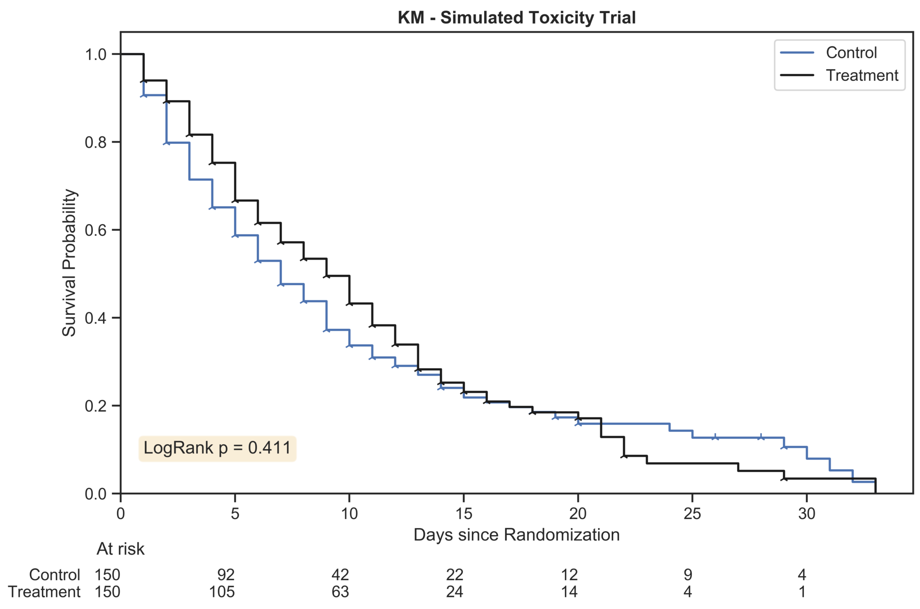
The Kaplan Meier estimator plot for a randomly generated chemotherapy toxicity trial of 300 patients with 1:1 allocation. An event was considered the onset of chemotherapy toxicity (beyond stage zero) and patients were censored once their assigned duration had been reached. The hazard ratio between treatment arms was 1.25:1.
Biomedinformatics 03 00052 g001
Figure 2. 
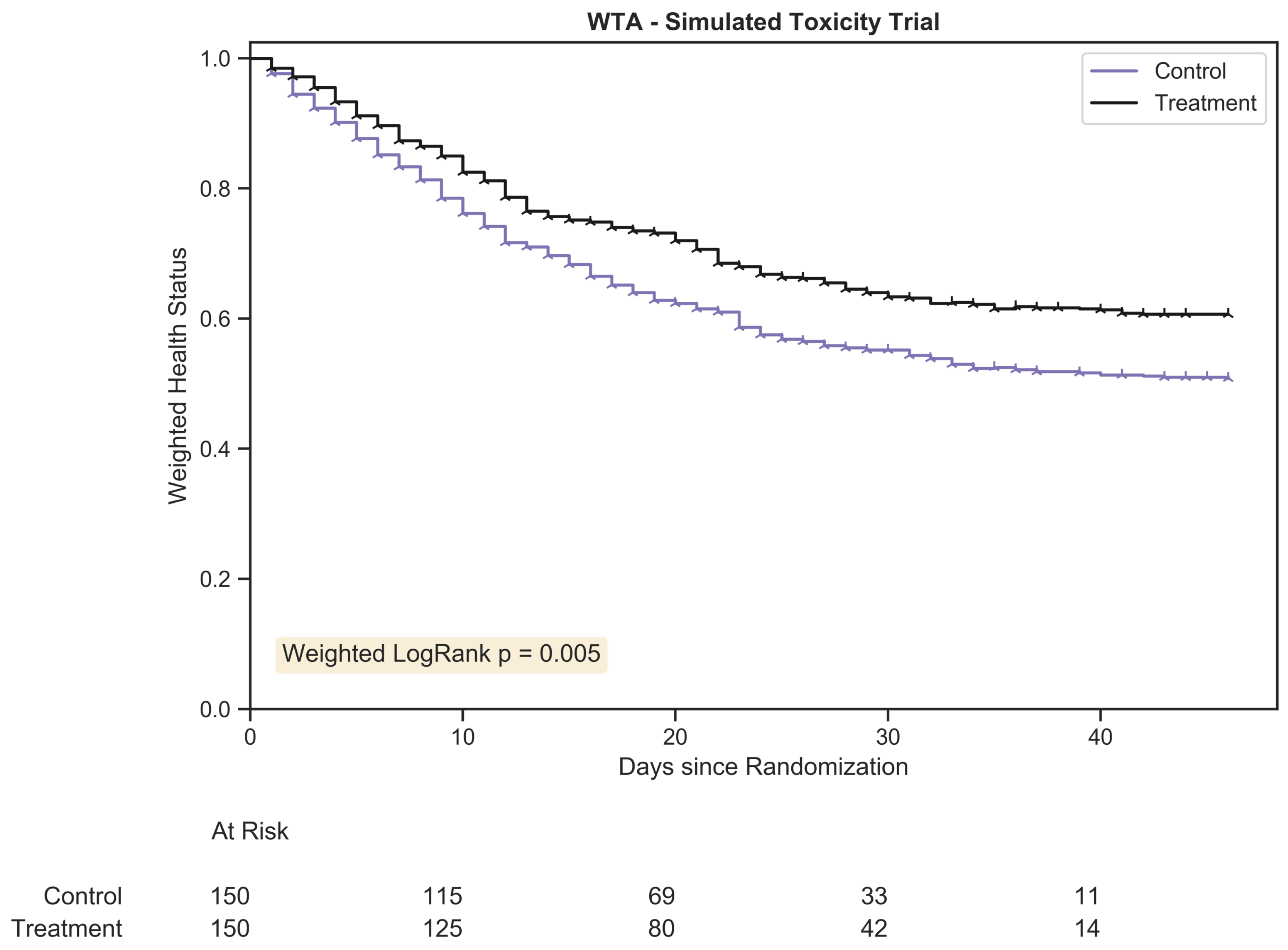
The weighted trajectory analysis plot for a randomly generated chemotherapy toxicity trial of 300 patients with 1:1 allocation. The weighted health status of both groups dropped due to increasing morbidity from chemotherapy toxicity following randomization. The hazard ratio between treatment arms was 1.25:1.
Biomedinformatics 03 00052 g002
Figure 3. 
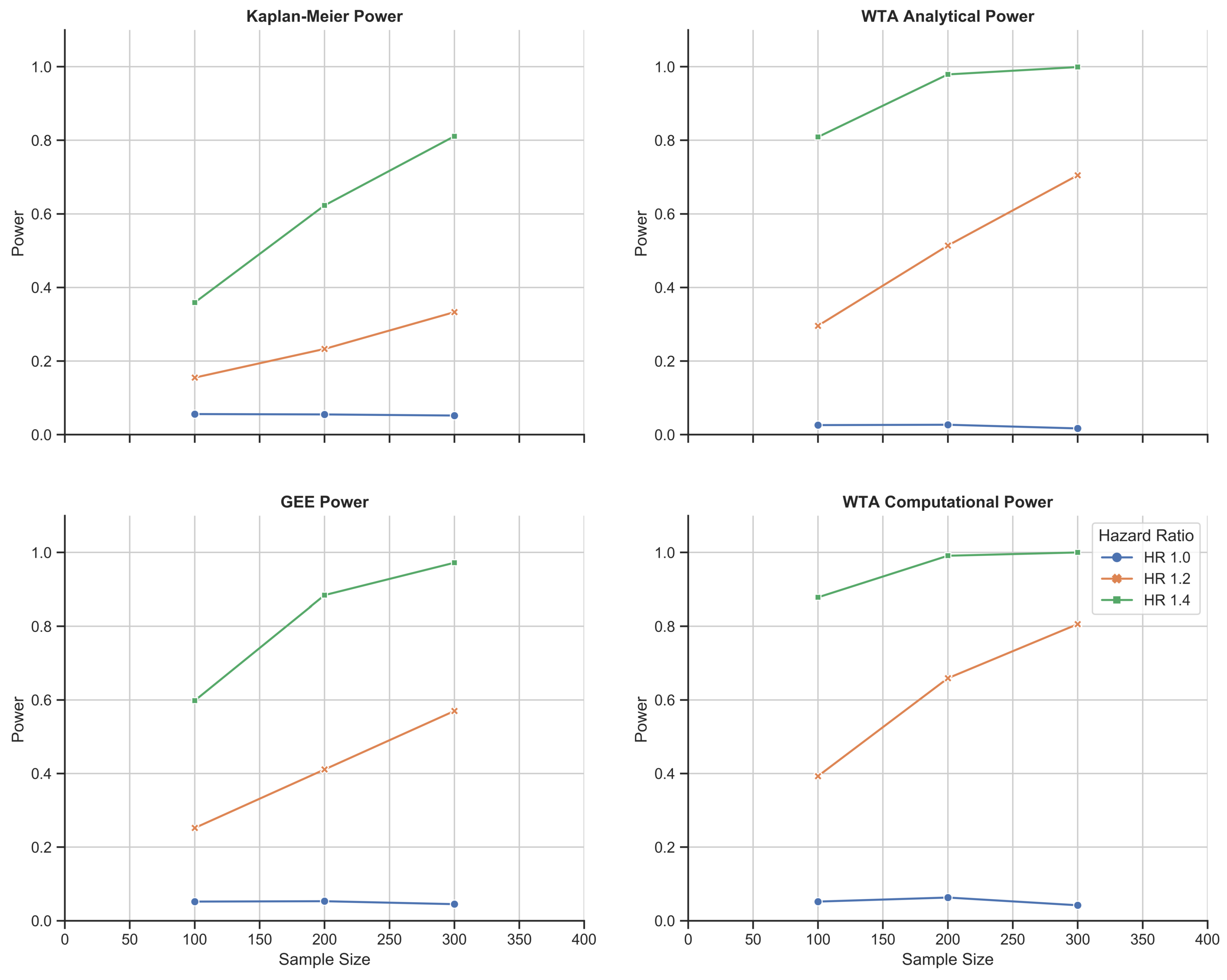
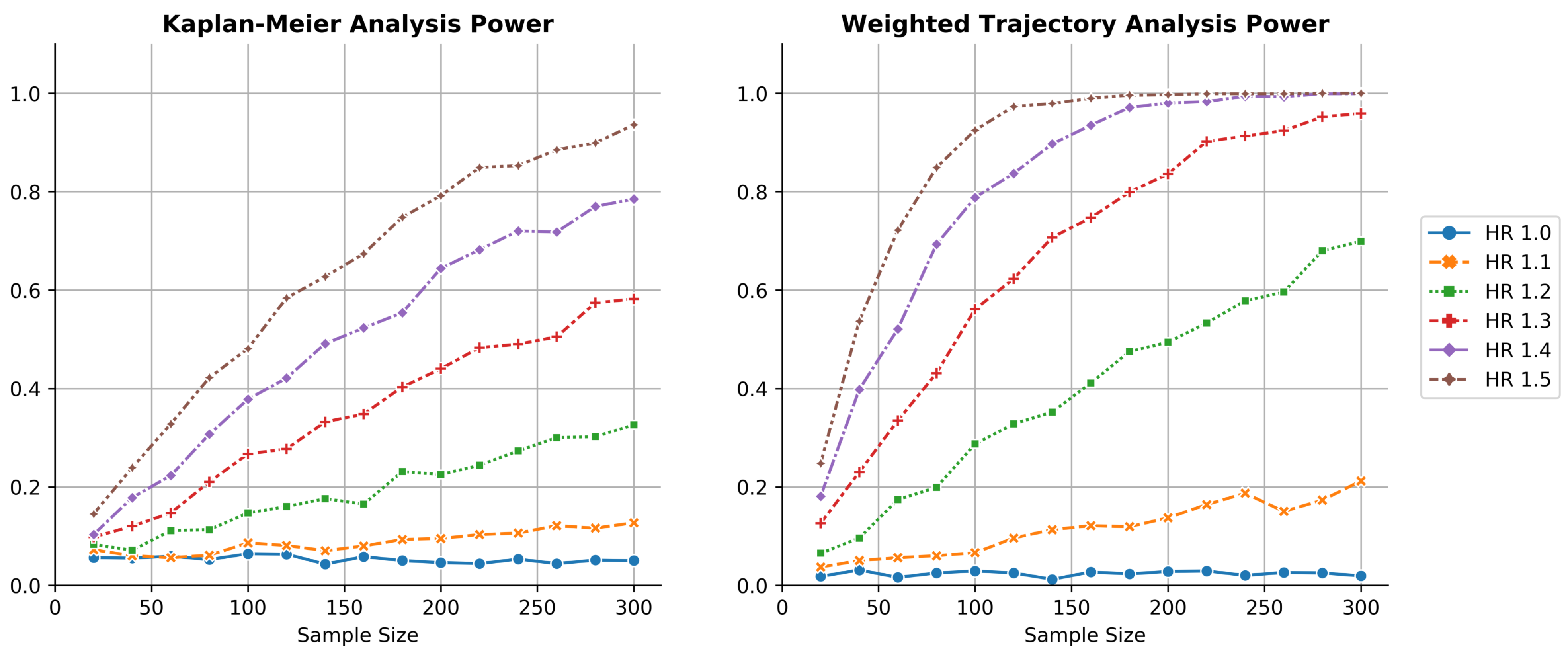
Thousandfold simulations of power as a function of sample size for both KM estimation and WTA across several hazard ratios. WTA demonstrated consistently higher power, reflecting a smaller sample size requirement during trial design. The type I error rate of WTA was approximately 0.025, indicating the method was conservative. The type I error approached 0.05 within the limit of larger trials with more distinct failure times.
Biomedinformatics 03 00052 g003
Figure 4. Chemotherapy toxicity simulation study: 1000-fold simulations of power as a function of sample size for KM estimation, the GEE, and WTA in both its analytical and computational forms. WTA outperformed KM estimation and the GEE with consistently higher power and, thus, a smaller sample size requirement. In addition, the computational approach with WTA outperformed the analytical approach in return for a more time- and resource-intensive methodology. The computational approach also met a standard type I error rate of 0.05 that was robust to changes in trial size.
Biomedinformatics 03 00052 g004
Figure 5. 
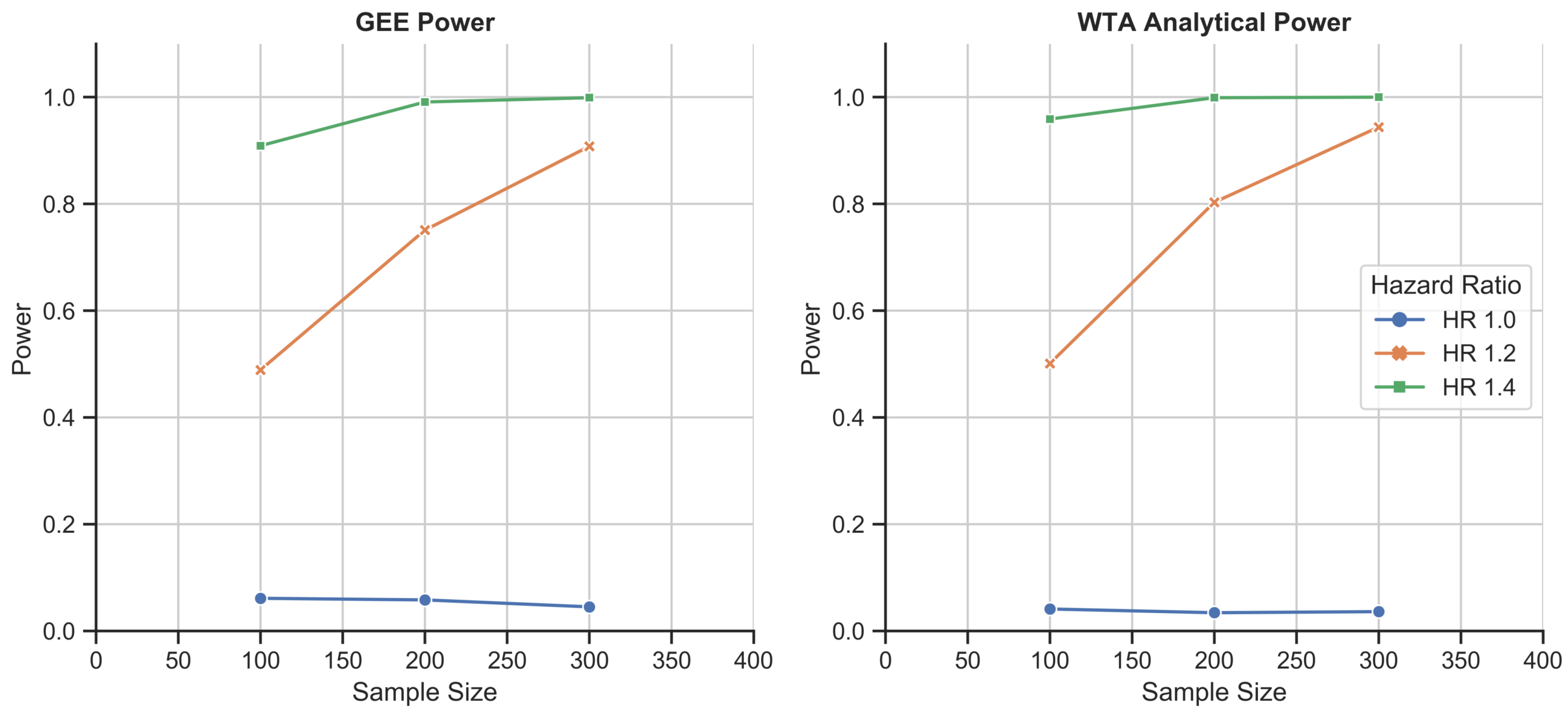
Schizophrenia disease course simulation study: 1000-fold simulations of power as a function of sample size for the GEE and WTA in its analytical form. WTA again outperformed the GEE and demonstrated a type I error rate of 0.037, closer to the 0.05 standard due to the larger size of each trial.
Biomedinformatics 03 00052 g005
Figure 6. 
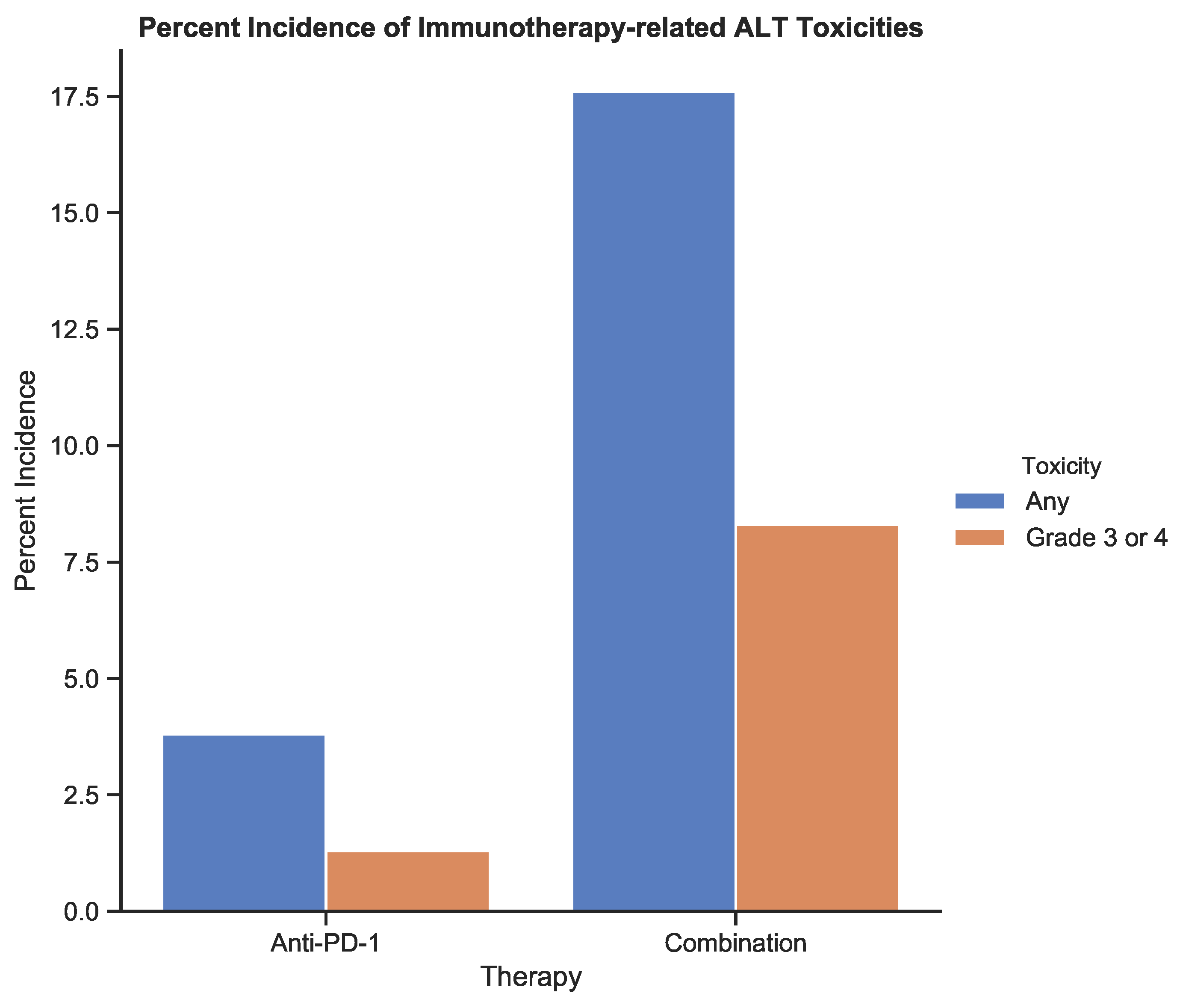
The incidence of treatment-related toxicities associated with an increase in alanine aminotransferase (ALT) for patients receiving anti-PD-1 therapy and combination therapy. Toxicities were graded using CTCAE v5.0 [6]. Data from Table 3 from the study by Larkin et al. (2015) [12].
Biomedinformatics 03 00052 g006
Figure 7. 
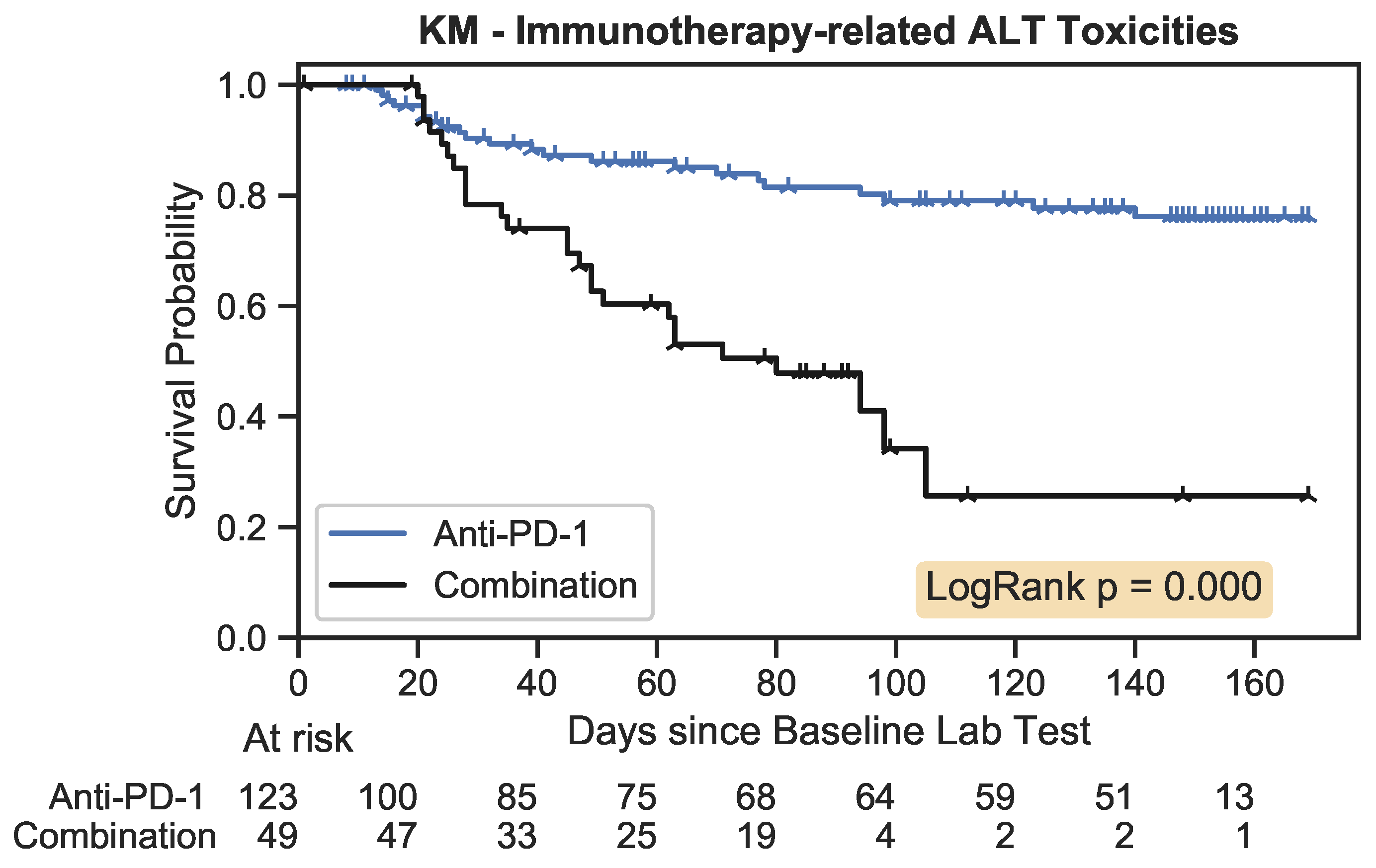
The Kaplan–Meier estimator plot for immunotherapy-related toxicities associated with an increase in ALT. An event was considered the onset of a nonzero toxicity grade.
Biomedinformatics 03 00052 g007
Figure 8. 
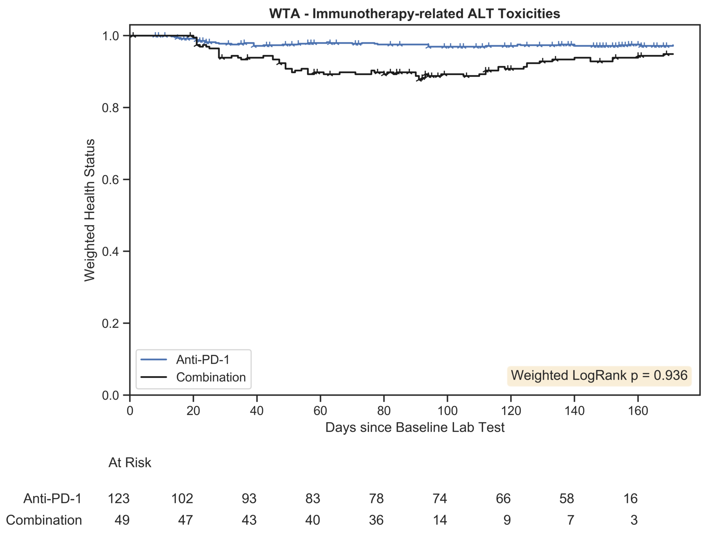
Weighted trajectory analysis plot for immunotherapy-related toxicities associated with an increase in ALT. The weighted health status of the combination group initially diverged from the anti-PD-1 group but subsequent recovery led to similar longitudinal outcomes.
Biomedinformatics 03 00052 g008
Figure 9. 
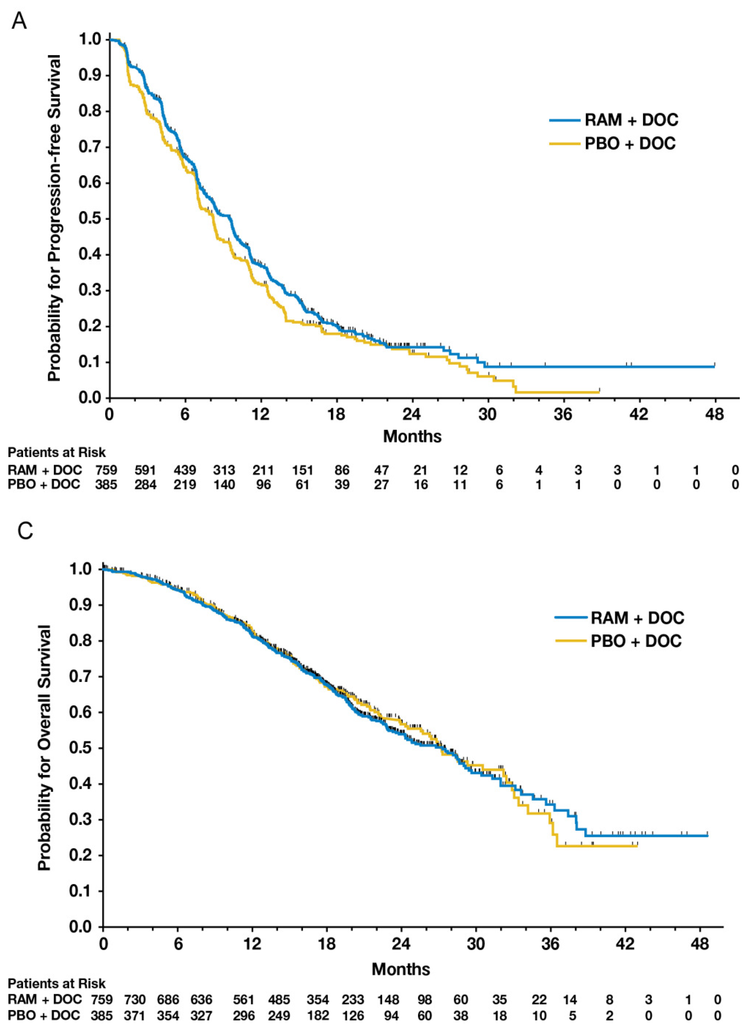
Figure 2A,C from Mackey et al.’s 2014 paper comparing ramucirumab to a placebo added to standard docetaxel chemotherapy [14]. The figures provide patient outcomes using KM estimates of progression-free survival (PFS) and overall survival (OS), respectively.
Biomedinformatics 03 00052 g009
Figure 10. 
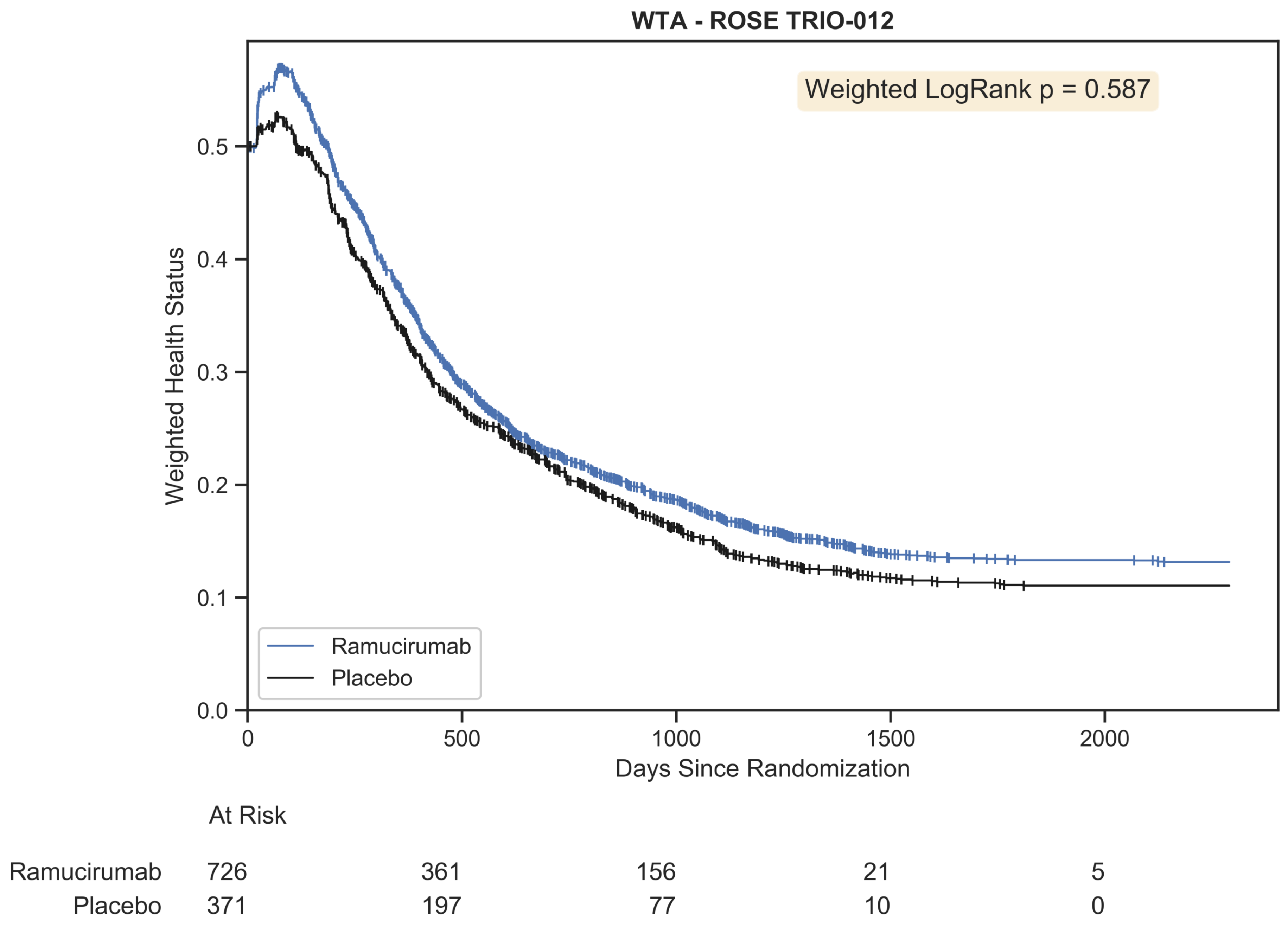
Weighted trajectory analysis of the original ROSE/TRIO-012 dataset using an ordinal scale that merges RECIST criteria with mortality. The trajectory of patient outcomes demonstrates that partial and complete response initially outweighed progressive disease and mortality for the first few chemotherapy cycles. Following this peak, patient prognosis was generally poor, as both treatment arms experienced growing disease burden and death.
Biomedinformatics 03 00052 g010
Table 1. Feature comparison between the Kaplan–Meier estimator and weighted trajectory analysis.
FeatureKaplan–Meier EstimatorWeighted Trajectory Analysis
EventOutcome with binary coding. A patient must begin at “0” and is removed from analysis following an event (“1”)An event is a change in clinical severity and does not remove a patient from further analysis. Must be discrete with a finite range that depends on the variable of interest
Variable of interestDeath, metastases, local recurrence, stroke, and more. Can include variables outside of medicine, such as postgraduate employmentGraded/staged outcomes: ECOG performance, toxicities, NYHA heart failure class, questionnaire scores, and more; also includes variables outside of medicine
TrajectorySurvival function always decreasesBidirectional: severity function can decrease or increase
CensoringRemoves patients from subsequent analysis (for withdrawal, discharge, loss to follow up, etc.)
Test for significanceLogrank testWeighted logrank test
Y-axisSurvival probabilityWeighted health status
X-axisTime (discrete: days, weeks, months, etc.)
Y-intercept1.0Between 0 and 1.0, inclusive
Weighted Trajectory Analysis, while retaining the serial time and censoring functionality of the Kaplan-Meier estimator, facilitates ordinal variables of interest and defines events as changes in severity that do not omit patients from subsequent analysis. In addition, the "weighted health status" is not a survival probability but rather a normalized aggregate score that dynamically falls with greater disease burden and increases with recovery.
Table 2. A snapshot of the final results of a simulated chemotherapy toxicity-grade trial.
Patient IDTreatment ArmDuration012345678910
11100000001110
21100000011111
301100000000000
416000000
501300000000011
619000000000
701800000011122
816000000
912900000000010
10040000
Treatment arms zero and one represent the control and treatment groups, respectively. Numbered columns indicate sequential days within the trial starting at day zero. Duration indicates the number of days the patient was hospitalized.
Table 4. RECIST 1.1 mapped to ordinal severity scores.
OutcomeScore
Complete response (CR)0
Partial response (PR)1
Stable disease (SD)2
Progressive disease (PD)3
Death4
Response Evaluation Criteria in Solid Tumours (RECIST) version 1.1 [15] adapted to Weighted Trajectory Analysis using ordinal severity scores. By convention, a score of zero is assigned to the lowest illness burden (complete response) and the maximum score to the highest illness burden (death).
Disclaimer/Publisher’s Note: The statements, opinions and data contained in all publications are solely those of the individual author(s) and contributor(s) and not of MDPI and/or the editor(s). MDPI and/or the editor(s) disclaim responsibility for any injury to people or property resulting from any ideas, methods, instructions or products referred to in the content.

