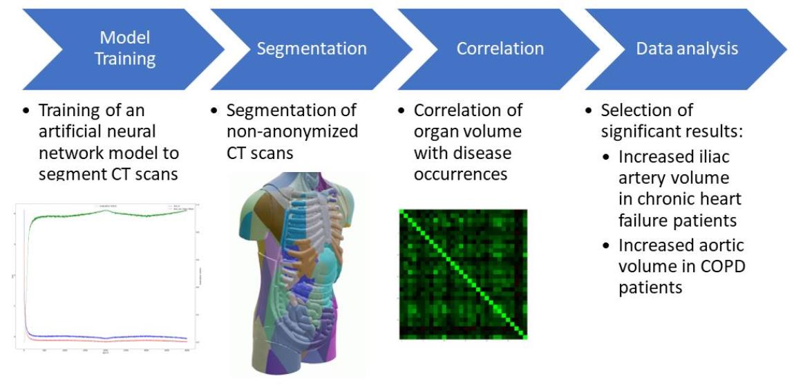
Improvement in Disease Diagnosis in Computed Tomography Images by Correlating Organ Volumes with Disease Occurrences in Humans

Abstract

Some diseases are known to cause or coincide with volume changes of certain structures in the body. Since these changes can be used to identify diseases, in this paper, we aimed to discover such new correlations. To this end, we trained a machine learning model based on the TotalSegmentator model on computed tomography (CT) image data, to segment 104 anatomical structures, while trying to improve the accuracy of the model. We then used the model to segment CT scans of decedents who had at least one of 18 diseases. After correlating the structure volumes with disease occurrences, a possible new correlation between chronic artery failure and iliac artery volume was found and others were confirmed. However, due to the limitations of the model and the underlying data, further research is required.

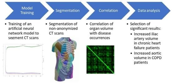
1. Introduction

The human body is an intricate network of cooperating structures and organs, which has not yet been fully explored. Diseases affecting one part of the body can thus have an effect on different, possibly otherwise unrelated parts of the body and may cause it to change. A simple and well-known example of this is spleen enlargement in patients with liver cirrhosis. This is due to the fact that when damaged tissue inside the liver blocks the blood flow coming from the portal vein, organs along the portal system, such as the spleen, experience higher blood pressure and increase in size and stiffness [1]. The coincidence of such changes with certain diseases may tell us more about the human body and may lead to improved diagnoses and treatment plans. To make further progress in this area, we looked at the distribution of volumes of anatomical structures, including bones, organs, large vessels, and large muscle groups, in patients with different diseases using computed tomography (CT) scans from patients who have a medical history of chronic or acute disease, and by correlating those disease markers with the volume of the aforementioned structures. During this work, we employed the TotalSegmentator model, which is an artificial neural network (ANN) [2], used for the segmentation of 104 anatomical structures [3], in order to support radiologists in evaluating radiological scan data. Additionally, we also attempted to improve the accuracy of the model by exploring different training parameters, such as the training duration and learning rate schedule. The 349 CT scans on which statistical analysis was performed were taken from the New Mexico Decedent Image Database (NMDID) [4], a database of postmortem CT scans routinely performed on decedents from New Mexico. The most common diseases among the patients are hypertension and diabetes type II. This arises from the way the data were chosen, since hypertension and diabetes type II are common among elderly people, which themselves are common in the NMDID, due to its nature as a database of scans of deceased individuals.

This kind of statistical analysis of organ sizes has previously not been conducted on this scale to our knowledge. New correlations can improve diagnostics by improving the diagnostic value of a CT scan and making it possible to recognize signs of diseases not originally checked for.

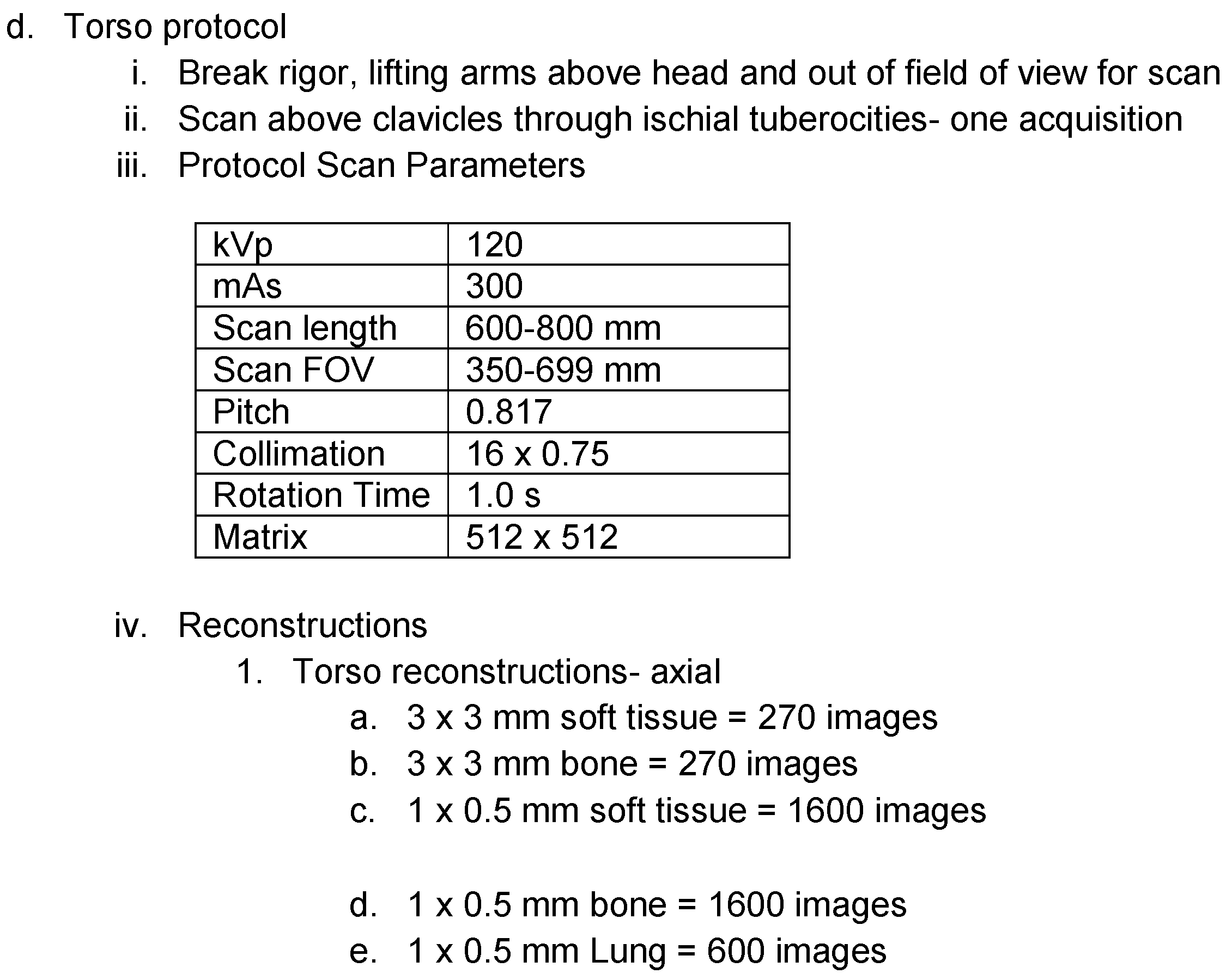
2. Materials and Methods

2.1. Model

The model used is a modified nnU-Net [5], a model and training framework developed by the MIC-DKFZ team, who aimed to develop a specialized model architecture for most medical segmentation tasks by automating decisions such as determining the patch size or number of layers for a given dataset. Its architecture is based on the U-Net [6]. The framework around the model was slightly modified into the TotalSegmentator model by the Department of Research and Analysis at University Hospital Basel, by disabling the benchmarking performed by the CUDA back end, which would have used a large amount of hardware resources when running inference [3]. Additionally, some training parameters such as training length and certain data augmentations were modified to improve the model accuracy. We built upon those changes and further explored different training lengths as well as learning rate schedules. The model uses the Nesterov-SGD learning rule, as this is the default optimizer for the nnU-Net [5].

2.2. Dataset for Model Training

The dataset used for training the TotalSegmentator model was a collection of 1204 CT scans of various body parts collected in several hospitals and clinics [3]. From the images, 104 anatomical structures, if present, were segmented, including bones, organs, muscle groups, and large blood vessels. A full list is included in

Table A1. Classes segmented by the TotalSegmentator model.

adrenal_gland_left	adrenal_gland_right	aorta
autochthon_left	autochthon_right	brain
clavicula_left	clavicula_right	colon
duodenum	esophagus	face
femur_left	femur_right	gallbladder
gluteus_maximus_left	gluteus_maximus_right	gluteus_medius_left
gluteus_medius_right	gluteus_minimus_left	gluteus_minimus_right
heart_atrium_left	heart_atrium_right	heart_myocardium
heart_ventricle_left	heart_ventricle_right	hip_left
hip_right	humerus_left	humerus_right
iliac_artery_left	iliac_artery_right	iliac_vena_left
iliac_vena_right	iliopsoas_left	iliopsoas_right
inferior_vena_cava	kidney_left	kidney_right
liver	lung_lower_lobe_left	lung_lower_lobe_right
lung_middle_lobe_right	lung_upper_lobe_left	lung_upper_lobe_right
pancreas	portal_vein_and_splenic_vein	pulmonary_artery
rib_left_1	rib_left_10	rib_left_11
rib_left_12	rib_left_2	rib_left_3
rib_left_4	rib_left_5	rib_left_6
rib_left_7	rib_left_8	rib_left_9
rib_right_1	rib_right_10	rib_right_11
rib_right_12	rib_right_2	rib_right_3
rib_right_4	rib_right_5	rib_right_6
rib_right_7	rib_right_8	rib_right_9
sacrum	scapula_left	scapula_right
small_bowel	spleen	stomach
trachea	urinary_bladder	vertebrae_C1
vertebrae_C2	vertebrae_C3	vertebrae_C4
vertebrae_C5	vertebrae_C6	vertebrae_C7
vertebrae_L1	vertebrae_L2	vertebrae_L3
vertebrae_L4	vertebrae_L5	vertebrae_T1
vertebrae_T10	vertebrae_T11	vertebrae_T12
vertebrae_T2	vertebrae_T3	vertebrae_T4
vertebrae_T5	vertebrae_T6	vertebrae_T7
vertebrae_T8	vertebrae_T9

. The segmentation was performed using a combination of existing models and board-certified radiologists, with radiologists correcting any mistakes in the segmentations produced by the models. Structures for which no model was available were segmented with a nnU-Net trained on the existing data. We modified a copy of the dataset by combining segmentations of the left and right versions of a body part, where those body parts would be mostly mirror images of each other. This was done to help the model recognize structures when applying data augmentation such as mirroring during the training. The 1204 images were split between a training dataset, a validation dataset, and a test dataset. The training dataset contained 1085 images, while the validation dataset contained 57 images. The test dataset contained 62 images. These were also the splits used in the original TotalSegmentator article, which is why they were used here. An example slice from the dataset can be found in Figure 1.

2.3. Dataset Used for Correlation

Since the dataset used for the model training had to be anonymized to be made public, no information regarding any potential diseases was included. Therefore, the data used in the second part of this paper were taken from the NMDID cases. The data from the NMDID consisted of 349 patient entries, with each entry consisting of two torso CT volumes, one optimized for soft tissue and the other for bone visualization. Example slices of a soft tissue-optimized scan can be found in Figure 2. The exact parameters used for the CT scan are listed in Figure A1. Prominent diagnoses in this dataset are hypertension (189 cases), diabetes type II (81 cases), and coronary artery disease (62 cases). A full list of diagnoses can be found in

Table A2. List of disease markers and their occurrences in the NMDID dataset.

Disease	Occurrences
Hypertension	181
Diabetes type II	73
Coronary artery disease	56
Hyperlipidemia	43
COPD	36
Asthma	33
Cirrhosis of the liver	31
Hepatitis C	28
Stroke	26
Diabetes type I	22
Arthritis	19
Chronic heart failure	18
Non-epileptic seizures	14
Autoimmune diseases	12
Myocardial infarction	12
Staphylococcus aureus	7
Osteoporosis	3
HIV/AIDS	3

.

2.4. Training

In all following equations, $lr$ is the learning rate for the current epoch $epoch$, while $l{r}_{max}$ is the maximal learning rate for the training, which occurs over $max\_epochs$ epochs. $pct$ represents the training progress and is defined as $epoch/max\_epochs$, while $peak$ refers to the proportion of $max\_epochs$ after which $l{r}_{max}$ is reached.

The model was trained on two NVIDIA RTX A6000 graphics cards using the data parallel method for 1000 epochs. The learning rate was scheduled with one of the following algorithms:

• Built-In: The built-in algorithm of the nnU-Net framework. The learning rate starts at the maximum learning rate and decreases polynomially using the formula

  $$lr=l{r}_{max}\times {(1-\frac{epoch}{max\_epochs})}^{0.9}.$$

  (1)
• Linear: The learning rate is varied cyclically over the course of training, rising linearly from zero to a maximal learning rate for the first part of a cycle, then decreasing linearly to zero during the second half of the cycle. The entire training consists of two cycles. When using this scheduler, the learning rate is cycled twice. The maximum learning rate is scheduled to be reached after half of the training. The practice of using multiple cycles was inspired by [7]. The formula for calculating the learning rate is

  $$lr=\left\{\begin{array}{cc}l{r}_{max}\times \frac{pct}{0.5}\hfill & ifpct\le 0.5\hfill \\ l{r}_{max}\times (1-\frac{pct}{0.5})\hfill & ifpct>0.5\hfill \end{array}\right..$$

  (2)
• Linear to Exponential: Modification of linear learning rate scheduling, which replaces the linear decrease in the second part with an exponential decrease, while only using one cycle. The maximum learning rate is scheduled to be reached after one quarter of the training. Here, the formula is

  $$lr=\left\{\begin{array}{cc}l{r}_{max}\times \frac{pct}{peak}\hfill & ifpct\le peak\hfill \\ l{r}_{max}\times e^{1-\frac{pct}{peak}}\hfill & ifpct>peak\hfill \end{array}\right..$$

  (3)
• Modified Linear to Exponential: To increase training efficiency in the early epochs and maintain greater training momentum during the second part of the training, we modified the learning rate schedule by taking the square root of the learning rate in the first part of training and decreasing the base from e to two for the exponential decay in the second half of the training. The modified formula is

  $$lr=\left\{\begin{array}{cc}l{r}_{max}\times \sqrt{\frac{pct}{peak}}\hfill & ifpct\le peak\hfill \\ l{r}_{max}\times 2^{1-\frac{pct}{peak}}\hfill & ifpct>peak\hfill \end{array}\right..$$

  (4)

3. Results

3.1. Network Training

The models were evaluated by calculating the Dice coefficient [5,8] between the predicted segmentations and the actual segmentations for the test part of the TotalSegmentator dataset. The Dice coefficients are listed in

Table 1. Dice coefficients of the different trained models on the test data of the TotalSegmentator dataset. The aggregate score is calculated by taking the average Dice coefficient for each class at the end of the training. Also listed is the mean Dice coefficient for all classes achieved by [5]. The learning rate schedulers are as given in Section 2.4. The “Opposing Labels” column states whether labels pertaining to similar versions of the same structure (e.g., left and right kidney) have been left separate or have been combined into one label containing all instances of the structure.

Opposing Labels	Learning Rate Scheduling	Epochs	Aggregate Score
Separate	Built-in	1000	0.9512
	Linear	4000	0.9611
	Linear to Exponential	1000	0.9491
	Quick Linear to Exponential	1000	0.9592
	Modified Linear to Exponential	1000	0.8850
Combined	Linear to Exponential	1000	0.9412
TotalSegmentator model		4000	greater than 0.96

. It is apparent that, while the training results did not surpass the results of the TotalSegmentator model, they were mostly close to the given lower bound. The Dice coefficient for the training with the modified linear to exponential learning rate scheduler is the lowest listed here.

Training times, including preprocessing and postprocessing for all images can be found in

Table 2. Average time elapsed per epoch for each of the models during training, in seconds. The first epoch was not included because of certain setup processes of the training script.

Opposing Labels	Learning Rate Scheduling	Epochs	Seconds per Epoch
Separate	Linear to Exponential	1000	332.2
	Linear	4000	712.1
	Quick Linear to Exponential	1000	668.7
	Modified Linear to Exponential	1000	649.4
	Built-in	1000	283.9
Combined	Modified	1000	624.8

.

3.2. Statistical Analysis

The volumes of the segmented structures were calculated by obtaining the voxel count for each segmented class and multiplying it by the volume per voxel in liters (dm${}^3$). Related structures (e.g., left and right kidney, ribs) were combined into a single structure for this. The sacrum was included in the vertebrae structure, as it is, for the purposes of this paper, an extension of the spine and not an independent structure. Some structures that did not fully appear in any image but still appeared as mistakes in the segmentation were removed from the data. Those structures include the brain, the face, and the vertebrae C1 through C6. A graph containing an overview of the volumes can be found in Figure A2. The average volumes and standard deviations for each structure are listed in

Table 3. Mean volume and standard deviation for each processed structure in liters (dm${}^3$).

Structure	Mean Volume	Standard Deviation	Variation Coefficient
Adrenal gland	0.0054	0.0028	0.5179
Aorta	0.0844	0.0502	0.5946
Autochton	1.0526	0.3078	0.2924
Clavicula	0.0537	0.0170	0.3166
Colon	1.5131	0.7031	0.4647
Duodenum	0.0336	0.0169	0.5029
Esophagus	0.0403	0.0145	0.3604
Femur	0.4747	0.1120	0.2358
Gluteal muscles	1.6934	0.5710	0.3372
Heart	0.3239	0.1251	0.3861
Hip	0.7445	0.1629	0.2189
Humerus	0.0877	0.0531	0.6056
Iliac artery	0.0119	0.0084	0.7093
Iliac vena	0.0212	0.0146	0.6903
Iliopsoas	0.5318	0.2042	0.3839
Inferior vena cava	0.0110	0.0108	0.9834
Kidney	0.2686	0.1013	0.3769
Liver	0.8613	0.4221	0.4901
Lung	2.6232	0.7547	0.2877
Pancreas	0.0214	0.0195	0.9088
Portal and splenic vein	0.0047	0.0043	0.9149
Pulmonary artery	0.0291	0.0167	0.5718
Ribs	0.4137	0.1127	0.2723
Scapula	0.2155	0.0520	0.2412
Small bowel	0.9991	0.4253	0.4257
Spleen	0.7638	0.2866	0.3752
Stomach	0.4096	0.2961	0.7229
Trachea	0.0210	0.0129	0.6145
Urinary bladder	0.1902	0.1832	0.9630
Vertebrae	0.9109	0.1684	0.1848

. After extracting the volumes, the Pearson correlation coefficient between the volumes of all pairs of structures was calculated (see

Table A3. Partial Pearson correlation coefficients between volumes of segmented and postprocessed structures and diseases of the NMDID dataset after accounting for all other data.

	Adrenal Gland	Aorta	Autochton	Clavicula	Colon	Duodenum
Adrenal gland	0.000	−0.049	0.075	−0.054	−0.085	−0.018
Aorta	−0.049	0.000	0.053	−0.054	−0.034	0.059
Autochton	0.075	0.053	0.000	−0.057	0.139	−0.041
Clavicula	−0.054	−0.054	−0.057	0.000	0.082	−0.045
Colon	−0.085	−0.034	0.139	0.082	0.000	0.154
Duodenum	−0.018	0.059	−0.041	−0.045	0.154	0.000
Esophagus	−0.047	−0.232	0.049	−0.068	0.215	−0.040
Femur	0.037	0.109	−0.261	−0.131	0.083	−0.085
Gluteal muscles	−0.010	−0.080	0.358	−0.031	0.120	0.038
Heart	0.130	0.029	−0.170	−0.043	−0.066	0.015
Hip	−0.014	−0.022	−0.142	0.018	−0.037	0.088
Humerus	0.029	−0.036	0.025	0.466	−0.030	0.087
Iliac artery	0.053	0.332	−0.016	−0.053	−0.030	0.106
Iliac vena	−0.108	0.257	−0.065	0.104	−0.002	0.059
Iliopsoas	−0.077	−0.086	0.417	−0.027	−0.118	−0.040
Inferior vena cava	−0.024	−0.050	−0.054	−0.046	0.118	0.052
Kidney	0.192	0.090	0.103	0.164	−0.142	−0.048
Liver	0.067	−0.045	0.004	−0.061	0.037	0.017
Lung	−0.090	0.168	0.100	−0.062	−0.085	0.000
Pancreas	0.110	0.066	−0.040	0.035	−0.343	0.201
Portal and splenic vein	0.123	0.010	0.000	−0.049	0.126	0.097
Pulmonary artery	0.065	0.117	0.108	0.076	−0.014	0.017
Ribs	−0.050	−0.103	0.145	0.045	−0.028	0.111
Scapula	0.093	0.089	0.116	0.428	−0.074	0.020
Small bowel	0.088	0.042	−0.004	−0.021	0.351	−0.090
Spleen	0.085	−0.014	0.120	0.015	0.020	0.053
Stomach	−0.057	0.084	0.097	−0.030	0.079	0.050
Trachea	−0.017	0.031	−0.060	0.004	0.083	−0.133
Urinary bladder	−0.088	−0.052	0.064	−0.000	−0.026	0.031
Vertebrae	0.017	0.105	0.103	0.044	0.092	−0.116
Diabetes type I	−0.024	0.003	0.003	−0.020	0.062	−0.034
Diabetes type II	0.121	−0.029	−0.039	0.103	0.019	0.020
COPD	−0.074	0.139	0.028	0.048	−0.116	0.016
Non−epileptic seizures	−0.012	0.071	0.058	−0.008	−0.027	−0.046
Asthma	−0.048	−0.023	0.021	−0.088	0.081	−0.027
Hypertension	0.097	0.066	−0.047	0.090	−0.024	−0.025
Arthritis	−0.012	0.021	−0.017	0.099	0.082	−0.085
Chronic heart failure	−0.024	−0.040	0.063	−0.058	0.091	−0.022
Stroke	0.039	0.040	−0.023	0.027	−0.014	−0.086
Myocardial infarction	0.030	−0.039	0.089	0.024	0.063	−0.012
Hyperlipidemia	−0.046	−0.033	−0.034	0.024	−0.066	0.019
HIV/AIDS	0.024	0.001	0.059	0.004	−0.028	−0.016
Hepatitis C	0.013	−0.012	−0.001	−0.012	−0.045	−0.056
Osteoporosis	0.006	−0.032	−0.035	−0.017	0.013	0.005
Cirrhosis of the liver	0.069	0.052	−0.004	0.085	−0.054	0.024
Coronary artery disease	−0.120	−0.095	−0.011	0.025	−0.009	0.033
Staphylococcus aureus	−0.006	0.092	−0.012	0.048	0.074	−0.185
Autoimmune diseases	0.064	−0.031	−0.007	0.065	−0.044	0.059
	Esophagus	Femur	Gluteal Muscles	Heart	Hip
Adrenal gland	−0.047	0.037	−0.010	0.130	−0.014
Aorta	−0.232	0.109	−0.080	0.029	−0.022
Autochton	0.049	−0.261	0.358	−0.170	−0.142
Clavicula	−0.068	−0.131	−0.031	−0.043	0.018
Colon	0.215	0.083	0.120	−0.066	−0.037
Duodenum	−0.040	−0.085	0.038	0.015	0.088
Esophagus	0.000	0.019	−0.003	0.074	0.038
Femur	0.019	0.000	0.148	0.014	0.296
Gluteal muscles	−0.003	0.148	0.000	0.014	0.163
Heart	0.074	0.014	0.014	0.000	−0.086
Hip	0.038	0.296	0.163	−0.086	0.000
Humerus	0.008	0.083	−0.055	−0.065	−0.020
Iliac artery	−0.038	0.103	−0.071	0.067	0.124
Iliac vena	0.096	0.013	0.060	0.199	0.125
Iliopsoas	−0.024	0.047	0.480	0.064	0.080
Inferior vena cava	−0.210	−0.180	0.010	−0.031	−0.061
Kidney	0.050	0.001	0.079	0.065	−0.017
Liver	−0.007	−0.094	0.016	0.092	0.019
Lung	0.206	−0.053	−0.202	0.075	0.063
Pancreas	0.086	0.033	0.030	−0.074	−0.090
Portal and splenic vein	0.107	−0.149	0.096	0.088	−0.047
Pulmonary artery	0.188	0.026	0.100	0.388	−0.055
Ribs	−0.089	0.167	−0.068	0.003	0.004
Scapula	0.108	0.083	−0.000	0.119	0.058
Small bowel	0.005	0.016	0.024	−0.060	−0.018
Spleen	0.176	−0.075	0.015	0.138	−0.021
Stomach	0.114	−0.065	0.125	0.116	−0.011
Trachea	0.109	−0.072	−0.087	0.021	−0.015
Urinary bladder	0.066	0.040	0.043	0.100	0.017
Vertebrae	−0.025	−0.076	0.013	0.008	0.536
Diabetes type I	0.185	−0.031	−0.080	−0.065	0.050
Diabetes type II	0.077	−0.040	−0.009	−0.016	0.070
COPD	0.018	0.131	0.101	−0.053	−0.074
Non−epileptic seizures	0.022	0.000	−0.025	0.079	0.026
Asthma	−0.049	0.001	0.006	−0.001	0.026
Hypertension	0.040	0.043	0.094	0.075	−0.117
Arthritis	0.032	0.054	0.019	0.006	0.040
Chronic heart failure	−0.092	−0.000	−0.005	0.154	−0.045
Stroke	0.091	−0.050	−0.110	−0.012	0.000
Myocardial infarction	0.042	0.071	0.011	0.129	−0.042
Hyperlipidemia	0.041	−0.023	0.038	−0.044	0.003
HIV/AIDS	0.012	0.121	0.018	0.114	−0.028
Hepatitis C	−0.026	0.029	0.029	0.091	−0.051
Osteoporosis	−0.014	−0.152	−0.041	−0.053	0.051
Cirrhosis of the liver	0.066	−0.004	−0.012	0.022	0.031
Coronary artery disease	−0.014	0.070	0.070	0.111	−0.104
Staphylococcus aureus	0.105	−0.055	−0.017	−0.020	0.025
Autoimmune diseases	0.055	0.102	0.000	0.028	−0.055
	Humerus	Iliac Artery	Iliac Vena	Iliopsoas	Inferior Vena Cava
Adrenal gland	0.029	0.053	−0.108	−0.077	−0.024
Aorta	−0.036	0.332	0.257	−0.086	−0.050
Autochton	0.025	−0.016	−0.065	0.417	−0.054
Clavicula	0.466	−0.053	0.104	−0.027	−0.046
Colon	−0.030	−0.030	−0.002	−0.118	0.118
Duodenum	0.087	0.106	0.059	−0.040	0.052
Esophagus	0.008	−0.038	0.096	−0.024	−0.210
Femur	0.083	0.103	0.013	0.047	−0.180
Gluteal muscles	−0.055	−0.071	0.060	0.480	0.010
Heart	−0.065	0.067	0.199	0.064	−0.031
Hip	−0.020	0.124	0.125	0.080	−0.061
Humerus	0.000	−0.036	−0.022	−0.019	0.056
Iliac artery	−0.036	0.000	0.173	−0.013	0.119
Iliac vena	−0.022	0.173	0.000	0.108	0.131
Iliopsoas	−0.019	−0.013	0.108	0.000	−0.013
Inferior vena cava	0.056	0.119	0.131	−0.013	0.000
Kidney	−0.023	−0.096	0.209	−0.068	0.154
Liver	−0.053	−0.135	0.127	−0.100	0.034
Lung	−0.028	−0.044	0.002	0.100	−0.048
Pancreas	−0.004	−0.018	0.127	0.104	0.079
Portal and splenic vein	0.097	0.066	0.030	−0.078	−0.104
Pulmonary artery	0.066	0.052	−0.065	−0.115	0.089
Ribs	−0.327	−0.052	−0.035	−0.032	0.066
Scapula	0.299	0.039	−0.013	0.133	−0.009
Small bowel	−0.051	0.178	−0.186	0.002	−0.016
Spleen	0.016	0.037	0.072	−0.079	−0.008
Stomach	−0.017	−0.100	0.100	−0.071	0.084
Trachea	0.034	0.040	−0.018	0.066	−0.063
Urinary bladder	−0.053	0.037	−0.149	−0.110	−0.015
Vertebrae	−0.063	0.044	−0.159	−0.126	0.180
Diabetes type I	0.023	0.021	−0.041	0.036	0.050
Diabetes type II	−0.037	0.049	−0.125	−0.041	0.025
COPD	0.052	0.065	−0.038	−0.107	−0.025
Non−epileptic seizures	0.053	−0.032	−0.075	−0.002	0.075
Asthma	−0.026	0.044	−0.016	0.003	0.002
Hypertension	−0.063	0.103	−0.061	−0.006	0.011
Arthritis	0.039	−0.042	0.001	0.012	0.094
Chronic heart failure	−0.066	0.137	0.007	−0.099	0.032
Stroke	0.104	0.018	0.082	0.055	−0.003
Myocardial infarction	−0.038	0.122	0.003	−0.062	0.040
Hyperlipidemia	−0.019	−0.032	0.026	−0.061	−0.015
HIV/AIDS	−0.026	−0.041	−0.052	−0.016	0.022
Hepatitis C	0.059	−0.028	0.039	−0.003	−0.003
Osteoporosis	−0.022	0.019	0.052	0.062	−0.062
Cirrhosis of the liver	−0.006	−0.045	−0.028	−0.071	−0.064
Coronary artery disease	0.004	0.170	−0.038	0.020	0.088
Staphylococcus aureus	−0.003	0.115	0.017	0.031	−0.027
Autoimmune diseases	0.028	0.009	0.016	0.015	−0.051
Adrenal gland	0.192	0.067	−0.090	0.110	0.123
Aorta	0.090	−0.045	0.168	0.066	0.010
Autochton	0.103	0.004	0.100	−0.040	0.000
Clavicula	0.164	−0.061	−0.062	0.035	−0.049
	Kidney	Liver	Lung	Pancreas	Portal and Splenic Vein
Colon	−0.142	0.037	−0.085	−0.343	0.126
Duodenum	−0.048	0.017	0.000	0.201	0.097
Esophagus	0.050	−0.007	0.206	0.086	0.107
Femur	0.001	−0.094	−0.053	0.033	−0.149
Gluteal muscles	0.079	0.016	−0.202	0.030	0.096
Heart	0.065	0.092	0.075	−0.074	0.088
Hip	−0.017	0.019	0.063	−0.090	−0.047
Humerus	−0.023	−0.053	−0.028	−0.004	0.097
Iliac artery	−0.096	−0.135	−0.044	−0.018	0.066
Iliac vena	0.209	0.127	0.002	0.127	0.030
Iliopsoas	−0.068	−0.100	0.100	0.104	−0.078
Inferior vena cava	0.154	0.034	−0.048	0.079	−0.104
Kidney	0.000	0.091	−0.042	−0.031	0.018
Liver	0.091	0.000	0.109	0.168	−0.125
Lung	−0.042	0.109	0.000	−0.193	0.057
Pancreas	−0.031	0.168	−0.193	0.000	0.239
Portal and splenic vein	0.018	−0.125	0.057	0.239	0.000
Pulmonary artery	−0.026	−0.060	−0.064	0.037	−0.087
Ribs	0.203	−0.076	0.198	0.091	0.028
Scapula	−0.142	0.109	0.038	−0.077	−0.064
Small bowel	0.209	0.247	−0.082	0.150	0.029
Spleen	0.121	0.173	−0.094	0.113	0.067
Stomach	0.084	−0.096	−0.030	0.147	−0.057
Trachea	−0.044	−0.106	0.078	0.042	−0.048
Urinary bladder	0.059	0.132	0.052	0.068	0.029
Vertebrae	−0.032	−0.008	0.122	0.075	0.040
Diabetes type I	0.112	0.051	−0.013	−0.060	−0.063
Diabetes type II	0.205	0.020	−0.006	0.055	−0.093
COPD	−0.017	−0.041	0.174	−0.029	0.018
Non−epileptic seizures	−0.014	−0.023	−0.115	−0.028	0.060
Asthma	0.003	−0.070	0.053	0.065	0.044
Hypertension	−0.148	−0.008	−0.075	−0.048	0.107
Arthritis	−0.049	0.044	0.003	−0.033	0.071
Chronic heart failure	−0.117	−0.035	−0.060	−0.046	0.015
Stroke	0.037	−0.003	0.020	0.120	−0.058
Myocardial infarction	0.001	−0.014	0.049	−0.003	−0.007
Hyperlipidemia	0.077	−0.094	0.037	0.013	−0.004
HIV/AIDS	−0.048	0.114	0.000	0.042	−0.017
Hepatitis C	−0.097	0.047	0.057	0.098	−0.014
Osteoporosis	0.067	0.016	0.080	−0.005	−0.050
Cirrhosis of the liver	0.258	0.097	0.031	0.096	−0.148
Coronary artery disease	−0.011	−0.059	−0.027	0.010	−0.003
Staphylococcus aureus	−0.092	0.110	0.044	−0.070	0.031
Autoimmune diseases	−0.036	0.028	−0.034	−0.028	−0.029
	Pulmonary Artery	Ribs	Scapula	Small Bowel	Spleen
Adrenal gland	0.065	−0.050	0.093	0.088	0.085
Aorta	0.117	−0.103	0.089	0.042	−0.014
Autochton	0.108	0.145	0.116	−0.004	0.120
Clavicula	0.076	0.045	0.428	−0.021	0.015
Colon	−0.014	−0.028	−0.074	0.351	0.020
Duodenum	0.017	0.111	0.020	−0.090	0.053
Esophagus	0.188	−0.089	0.108	0.005	0.176
Femur	0.026	0.167	0.083	0.016	−0.075
Gluteal muscles	0.100	−0.068	−0.000	0.024	0.015
Heart	0.388	0.003	0.119	−0.060	0.138
Hip	−0.055	0.004	0.058	−0.018	−0.021
Humerus	0.066	−0.327	0.299	−0.051	0.016
Iliac artery	0.052	−0.052	0.039	0.178	0.037
Iliac vena	−0.065	−0.035	−0.013	−0.186	0.072
Iliopsoas	−0.115	−0.032	0.133	0.002	−0.079
Inferior vena cava	0.089	0.066	−0.009	−0.016	−0.008
Kidney	−0.026	0.203	−0.142	0.209	0.121
Liver	−0.060	−0.076	0.109	0.247	0.173
Lung	−0.064	0.198	0.038	−0.082	−0.094
Pancreas	0.037	0.091	−0.077	0.150	0.113
Portal and splenic vein	−0.087	0.028	−0.064	0.029	0.067
Pulmonary artery	0.000	−0.051	−0.131	−0.010	−0.013
Ribs	−0.051	0.000	0.408	0.059	0.007
Scapula	−0.131	0.408	0.000	0.113	−0.038
Small bowel	−0.010	0.059	0.113	0.000	−0.017
Spleen	−0.013	0.007	−0.038	−0.017	0.000
Stomach	0.162	0.026	0.001	0.155	−0.364
Trachea	0.037	−0.018	0.049	−0.100	−0.025
Urinary bladder	−0.042	0.042	0.011	−0.114	0.026
Vertebrae	0.145	0.212	0.183	−0.044	0.079
Diabetes type I	−0.037	−0.089	−0.013	0.059	−0.013
Diabetes type II	−0.055	0.011	−0.081	0.076	−0.060
COPD	0.043	−0.061	−0.119	0.055	0.040
Non−epileptic seizures	−0.042	0.091	−0.073	0.009	0.025
Asthma	0.075	−0.032	0.112	−0.092	0.029
Hypertension	−0.031	−0.002	−0.035	−0.011	0.040
Arthritis	0.002	0.014	−0.172	0.099	−0.026
Chronic heart failure	−0.038	0.029	0.167	−0.072	0.111
Stroke	−0.041	0.136	−0.154	0.014	−0.156
Myocardial infarction	−0.052	−0.045	0.021	0.013	−0.049
Hyperlipidemia	−0.045	−0.012	0.010	0.065	0.004
HIV/AIDS	−0.007	−0.042	−0.063	−0.023	−0.053
Hepatitis C	−0.090	0.049	−0.022	0.081	−0.035
Osteoporosis	0.050	−0.042	0.035	−0.010	−0.038
Cirrhosis of the liver	−0.078	−0.022	−0.074	0.135	−0.266
Coronary artery disease	−0.019	0.033	−0.058	−0.085	0.001
Staphylococcus aureus	−0.058	0.012	−0.007	0.047	0.005
Autoimmune diseases	−0.096	−0.052	−0.136	0.004	−0.043
	Stomach	Trachea	Urinary Bladder	Vertebrae
Adrenal gland	−0.057	−0.017	−0.088	0.017
Aorta	0.084	0.031	−0.052	0.105
Autochton	0.097	−0.060	0.064	0.103
Clavicula	−0.030	0.004	−0.000	0.044
Colon	0.079	0.083	−0.026	0.092
Duodenum	0.050	−0.133	0.031	−0.116
Esophagus	0.114	0.109	0.066	−0.025
Femur	−0.065	−0.072	0.040	−0.076
Gluteal muscles	0.125	−0.087	0.043	0.013
Heart	0.116	0.021	0.100	0.008
Hip	−0.011	−0.015	0.017	0.536
Humerus	−0.017	0.034	−0.053	−0.063
Iliac artery	−0.100	0.040	0.037	0.044
Iliac vena	0.100	−0.018	−0.149	−0.159
Iliopsoas	−0.071	0.066	−0.110	−0.126
Inferior vena cava	0.084	−0.063	−0.015	0.180
Kidney	0.084	−0.044	0.059	−0.032
Liver	−0.096	−0.106	0.132	−0.008
Lung	−0.030	0.078	0.052	0.122
Pancreas	0.147	0.042	0.068	0.075
Portal and splenic vein	−0.057	−0.048	0.029	0.040
Pulmonary artery	0.162	0.037	−0.042	0.145
Ribs	0.026	−0.018	0.042	0.212
Scapula	0.001	0.049	0.011	0.183
Small bowel	0.155	−0.100	−0.114	−0.044
Spleen	−0.364	−0.025	0.026	0.079
Stomach	0.000	−0.074	0.023	−0.063
Trachea	−0.074	0.000	0.156	0.133
Urinary bladder	0.023	0.156	0.000	−0.039
Vertebrae	−0.063	0.133	−0.039	0.000
Diabetes type I	−0.034	−0.029	0.056	0.017
Diabetes type II	−0.054	0.024	0.099	−0.047
COPD	0.004	−0.111	−0.124	0.102
Non−epileptic seizures	0.024	0.063	0.116	−0.085
Asthma	0.021	−0.077	−0.037	−0.135
Hypertension	0.034	−0.086	−0.022	0.121
Arthritis	−0.087	0.036	−0.001	0.009
Chronic heart failure	0.055	0.018	0.072	−0.070
Stroke	−0.105	−0.068	0.057	0.053
Myocardial infarction	−0.150	−0.028	−0.051	−0.035
Hyperlipidemia	0.010	−0.054	−0.030	−0.004
HIV/AIDS	−0.047	0.094	−0.014	0.064
Hepatitis C	−0.071	−0.034	−0.025	0.020
Osteoporosis	−0.040	0.050	−0.013	−0.027
Cirrhosis of the liver	−0.128	−0.000	0.108	−0.048
Coronary artery disease	−0.011	−0.062	−0.052	0.048
Staphylococcus aureus	−0.002	−0.135	0.025	−0.033
Autoimmune diseases	0.112	−0.090	−0.001	0.160

). Correlation coefficients were also calculated between each disease marker and the volume of each structure. These can also be found in Table A3. Correlation coefficients between volumes exceeding 0.5 are listed in

Table 4. Pearson correlation coefficients (r) exceeding 0.5 between structure volumes.

Structures		r	p-Value
Hip	Vertebrae	0.7353	<0.05
Autochthon	Gluteal muscles	0.7116	<0.05
Iliopsoas	Gluteal muscles	0.7102	<0.05
Autochthon	Iliopsoas	0.6829	<0.05
Scapula	Ribs	0.6481	<0.05
Scapula	Vertebrae	0.6076	<0.05
Clavicula	Scapula	0.5979	<0.05
Hip	Scapula	0.5974	<0.05
Ribs	Vertebrae	0.5954	<0.05
Hip	Ribs	0.5917	<0.05
Scapula	Autochthon	0.5044	<0.05
Clavicula	Humerus	0.5003	<0.05

. Correlation coefficients between structure volumes and diseases mostly did not exceed 0.2. The only exceptions to this were between chronic heart failure and iliac artery volume (r = 0.238, p < 0.001) and between aorta volume and chronic obstructive pulmonary disease (COPD), with r = 0.228.

The partial correlation coefficients also mostly did not exceed an absolute value of 0.2. The only exceptions to this were between spleen volume and liver cirrhosis (r = −0.267, p < 0.001), kidney volume and liver cirrhosis (r = 0.257, p < 0.001), and kidney volume and diabetes type II (r = 0.205, p < 0.001).

4. Discussion

4.1. Network Training

Training losses were mostly slightly below those reported by [3], indicating no significant improvements in segmentation quality. One exception was training with the modified linear to exponential learning rate scheduler (see Section 2.4 and Table 1). Here, the final Dice coefficient at the end of training was 0.88496, indicating a poor suitability for training this network compared with the other schedulers. Another exception was the model trained with the Linear learning rate scheduler, which was the only model to reach a final Dice coefficient of more than 0.96, as the TotalSegmentator model. This was the only scheduler to use more than two cycles, and it was also the scheduler with the longest run time. This may indicate that the overfitting point of the training may not have been reached and that a longer training may further improve results. This also indicates that multiple cycles might help the net generalize better.

Regarding the inference and training times of the trained models, despite the high computational cost needed for segmentation, the Dice score was around 0.95 for most models, indicating that it performs well while ideally introducing only limited inaccuracies. Even when taking into account the time needed to correct these errors, evaluating the model still saves time compared to manual segmentation. It may be possible to reduce the hardware footprint (including inference times) of the algorithm by rerunning the configuration and training on a less powerful device, as the nnU-Net configurator by default tries to use as much of the available processing power as possible, leading to a strong hardware dependency if trained on very powerful hardware. By using less powerful hardware, not only would the memory footprint of the model decrease, but so would the inference time, due to a smaller and simpler model.

4.2. Statistical Analysis-Simple Correlation Coefficients

The highest correlations between volumes, as seen in Table 4, were between certain bones and muscle groups, which is to be expected, given that the human body tends to grow proportionally.

The correlation between chronic heart failure and iliac artery volume has not previously been described in the literature to the best of our knowledge. This may have been caused by an overrepresentation of hypertension in the underlying data, a known cause of heart failure, as well as of enlarged blood vessels. This overrepresentation could have led to an increased number of cases with enlarged vessels, as well as heart failures. Additionally, the patients were scanned after rigor mortis had subsided, allowing the muscles in the vessel walls to relax and possibly distend. Another explanation for this correlation, however, is that the segmentation of the iliac arteries was qualitatively inferior, causing random variations in the volume data to appear as correlations. This hypothesis is supported by the fact that the TotalSegmentator also had problems segmenting the iliac artery and vein [3]. In addition, the data from the NMDID had a significantly different contrast level compared to the data the model was trained on (compare Figure 1 and Figure 2). This difference put the NMDID data outside of the data distribution on which the model was trained, which also decreased the segmentation quality. These factors may have compounded, to result in the irregular segmentation shape also seen in Figure A2, where the volumes for the iliac artery and vein do not seem to be normally distributed. The variation coefficient was also rather high, with values of 0.709 and 0.690 for the iliac artery and vein, respectively. The p-value of this correlation was however very small (p < 0.001), indicating only a very small probability that this correlation was not found in the obtained data. Further research, including better volume data, is needed.

The second notable correlation, between occurrences of COPD and aorta volume, has previously been described by [9], who made no claims about causality or temporality, due to the limitations of their study. Since this paper is also limited by the fact that the used CT scans were postmortem, no claims regarding causality or temporality can be made here either. There may, however, be a common cause for these two conditions, since endothelial damage and a decrease in elastin and collagen is a cause of aortic wall degradation, as well as emphysema, which is a major part of COPD [9,10].

4.3. Statistical Analysis-Partial Correlation Coefficients

The positive correlation between kidney size and diabetes type II fits with current medical knowledge about kidney hypertrophy in patients with diabetes, and more specifically diabetic nephropathy [11]. With diabetes type I, this connection was also somewhat observed in the data, with a slightly positive coefficient (r = 0.112); it was, however, weaker than the correlation with diabetes type II. This might have simply been due to the inferior quality of the predicted volumes or statistical variation due to a smaller sample size of patients with diabetes type I (n = 23).

The slight positive correlation between kidney size and liver cirrhosis also fits with current medical knowledge. Both the kidneys and the liver are responsible for regulating blood composition. In cases of liver failure, the kidneys may compensate by increasing filtering activity, which is accompanied by an increase in volume [12].

The slightly negative correlation between spleen size and liver cirrhosis is contrary to established medical knowledge. Usually, in cases of liver cirrhosis, the spleen should show an increase in size [1]; however, this correlation suggests that, in our cases, the spleen tended to have a smaller volume in cases with liver cirrhosis. This inaccuracy in our data may have again been caused by inaccurate volume data. However, the p-value was again very small (p < 0.0001), hinting that there might have been a problem with the model when segmenting enlarged spleens. Possibly, this came from the training dataset not including cases with spleen enlargement, which would put enlarged spleens outside of the patterns the model had learned to recognize, causing the model to segment the spleen incorrectly.

4.4. Conclusions

The neural network training produced models that were reasonably accurate but that require powerful hardware to run. The statistical analysis of organ volumes yielded a previously undescribed correlation between chronic heart failure and iliac artery size, and confirmed a correlation between liver cirrhosis and kidney size, as well as a correlation between aorta volume and COPD. Due to the low correlation coefficients and difficulties in segmenting the NMDID data, further research is required to confirm the results.

4.5. Outlook

Due to the long training times, only a small part of the possible nnU-Net configurations could be explored. Future work may, thus, be dedicated to improving the model by exploring more model configurations. Currently, however, the segmentations produced by the model show inaccuracies when segmenting small soft tissue structures, such as the spleen, smaller vessels, or the heart (apparent in the high variation coefficients in Table 3).

The data correlation yielded mixed results. No new strong correlations were found, and the weak correlations that were found require further research. Future work may focus on trying to replicate the correlation between iliac vessel size and chronic heart failure with higher quality segmentations or, since perfect segmentation results are highly unlikely to ever be achieved, higher quality volume data from other sources. Another problem with the dataset was its limited size, as most diseases occurred in less than 40 cases. Additionally, about half of the cases had two or more disease markers. This leads to problems isolating possible effects of diseases. This could be mitigated by using a larger dataset with more patients and a better disease distribution, as well as by including healthy patients for comparison.

References

- Takuma, Y.; Nouso, K.; Morimoto, Y.; Tomokuni, J.; Sahara, A.; Takabatake, H.; Matsueda, K.; Yamamoto, H. Portal Hypertension in Patients with Liver Cirrhosis: Diagnostic Accuracy of Spleen Stiffness. Radiology 2016, 279, 609–619. [Google Scholar] [CrossRef] [PubMed]
- Egger, J.; Gsaxner, C.; Pepe, A.; Pomykala, K.L.; Jonske, F.; Kurz, M.; Li, J.; Kleesiek, J. Medical deep learning—A systematic meta-review. Comput. Methods Programs Biomed. 2022, 221, 106874. [Google Scholar] [CrossRef] [PubMed]
- Wasserthal, J.; Meyer, M.; Breit, H.C.; Cyriac, J.; Yang, S.; Segeroth, M. TotalSegmentator: Robust segmentation of 104 anatomical structures in CT images. arXiv 2022, arXiv:2208.05868. [Google Scholar] [CrossRef]
- Edgar, H.; Daneshvari Berry, S.; Moes, E.; Adolphi, N.; Bridges, P.; Nolte, K. New Mexico Decedent Image Database; Office of the Medical Investigator, University of New Mexico: Albuquerque, NM, USA, 2020. [Google Scholar] [CrossRef]
- Isensee, F.; Jaeger, P.F.; Kohl, S.A.A.; Petersen, J.; Maier-Hein, K.H. nnU-Net: A self-configuring method for deep learning-based biomedical image Segmentation. Nat. Methods 2020, 18, 203–211. [Google Scholar] [CrossRef] [PubMed]
- Ronneberger, O.; Fischer, P.; Brox, T. U-Net: Convolutional Networks for Biomedical Image Segmentation. In Proceedings of the Medical Image Computing and Computer-Assisted Intervention (MICCAI), Munich, Germany, 5–9 October 2015; LNCS; Springer: Berlin/Heidelberg, Germany, 2015; Volume 9351, pp. 234–241. [Google Scholar] [CrossRef]
- Smith, L.N. Cyclical Learning Rates for Training Neural Networks. In Proceedings of the 2017 IEEE Winter Conference on Applications of Computer Vision (WACV), Santa Rosa, CA, USA, 24–31 March 2017. [Google Scholar] [CrossRef]
- Egger, J.; Kapur, T.; Fedorov, A.; Pieper, S.; Miller, J.V.; Veeraraghavan, H.; Freisleben, B.; Golby, A.J.; Nimsky, C.; Kikinis, R. GBM volumetry using the 3D Slicer medical image computing platform. Sci. Rep. 2013, 3, 1–7. [Google Scholar] [CrossRef] [PubMed]
- Fujikura, K.; Albini, A.; Barr, R.G.; Parikh, M.; Kern, J.; Hoffman, E.; Hiura, G.T.; Bluemke, D.A.; Carr, J.; Lima, J.A.; et al. Aortic enlargement in chronic obstructive pulmonary disease (COPD) and emphysema: The Multi-Ethnic Study of Atherosclerosis (MESA) COPD study. Int. J. Cardiol. 2021, 331, 214–220. [Google Scholar] [CrossRef] [PubMed]
- Snider, G.L.; Kleinerman, J.; Thurlbeck, W.M.; Bengali, Z.H. The Definition of Emphysema. Am. Rev. Respir. Dis. 1985, 132, 182–185. [Google Scholar]
- Habib, S.L. Kidney atrophy vs hypertrophy in diabetes: Which cells are involved? Cell Cycle 2018, 17, 1683–1687. [Google Scholar] [CrossRef] [PubMed]
- Saad, M.; Ellis, C.L.; O’Neill, W.C. Renal Hypertrophy in Liver Failure. Kidney Int. Rep. 2018, 3, 1464–1467. [Google Scholar] [CrossRef] [PubMed]
- Office of the Medical Investigator-UNM. Available online: https://hsc.unm.edu/omi/ (accessed on 18 May 2023).
- CT Scan Protocol. Available online: https://nmdid.unm.edu/resources/data-information (accessed on 18 May 2023).
- Torso Protocol. Available online: https://nmdid.unm.edu/docs/CT_OMI_protocol.pdf (accessed on 18 May 2023).