Article

A Segmented Weighting and Elimination Method for GNSS Diffraction Errors in Urban Building Obstruction Environments

1
Wuhan Municipal Construction Group Co., Ltd., Wuhan 430080, China
2
Wuhan Municipal Environmental Engineering Construction Co., Ltd., Wuhan 430080, China
3
School of Civil Engineering and Architecture, Wuhan University of Technology, 122 Luoshi Road, Wuhan 430070, China
4
China Three Gorges Construction Engineering Corporation, Chengdu 610095, China
*
Author to whom correspondence should be addressed.
Geomatics 2026, 6(3), 58; https://doi.org/10.3390/geomatics6030058
Submission received: 1 April 2026 / Revised: 30 April 2026 / Accepted: 8 May 2026 / Published: 1 June 2026

Highlights

What are the main findings?
  • Diffraction error is strongly correlated with the carrier-power-to-noise-density ratio (C/N0), and the C/N0 time series is consistent with the theoretically predicted growth pattern of diffraction error.
  • This study proposes a GNSS diffraction error mitigation approach involving segmented down-weighting and elimination of affected observations.
What are the implications of the main findings?
  • C/N0 can serve as a practical indicator of diffraction-affected signals, enabling adaptive down-weighting or exclusion according to error severity.
  • The proposed method effectively mitigates diffraction errors and substantially improves ambiguity-fixing performance and positioning accuracy in dense urban environments.

Abstract
In densely built urban environments, GNSS signals frequently undergo diffraction at building edges, and the resulting errors can severely degrade positioning accuracy and reliability. Previous studies have shown a strong correlation between diffraction error and the carrier-power-to-noise-density ratio (C/N0). Building on this observation, this study proposes a GNSS diffraction-mitigation method based on segmented down-weighting and exclusion of affected observations. First, an open-sky reference model of the elevation–C/N0 relationship is established for each satellite class. A robust strategy is then introduced to adaptively down-weight moderately contaminated observations and remove severely affected ones during stochastic modeling. The proposed method is evaluated using both static and kinematic datasets collected in dense urban environments. In the static experiment under severe building obstruction, the ambiguity-fixing rate (AFR) reaches 95.5%, with horizontal and vertical accuracies of 4 mm and 8 mm, respectively, substantially outperforming conventional weighting strategies. In the vehicle-based kinematic experiment, the fixed-solution rate exceeds 80%, and the float solution is also noticeably improved relative to traditional weighting and exclusion methods. Overall, the proposed method effectively mitigates diffraction-induced errors and improves positioning performance in dense urban environments, with potential applications in automated inspection, intelligent construction, and high-precision deformation monitoring.

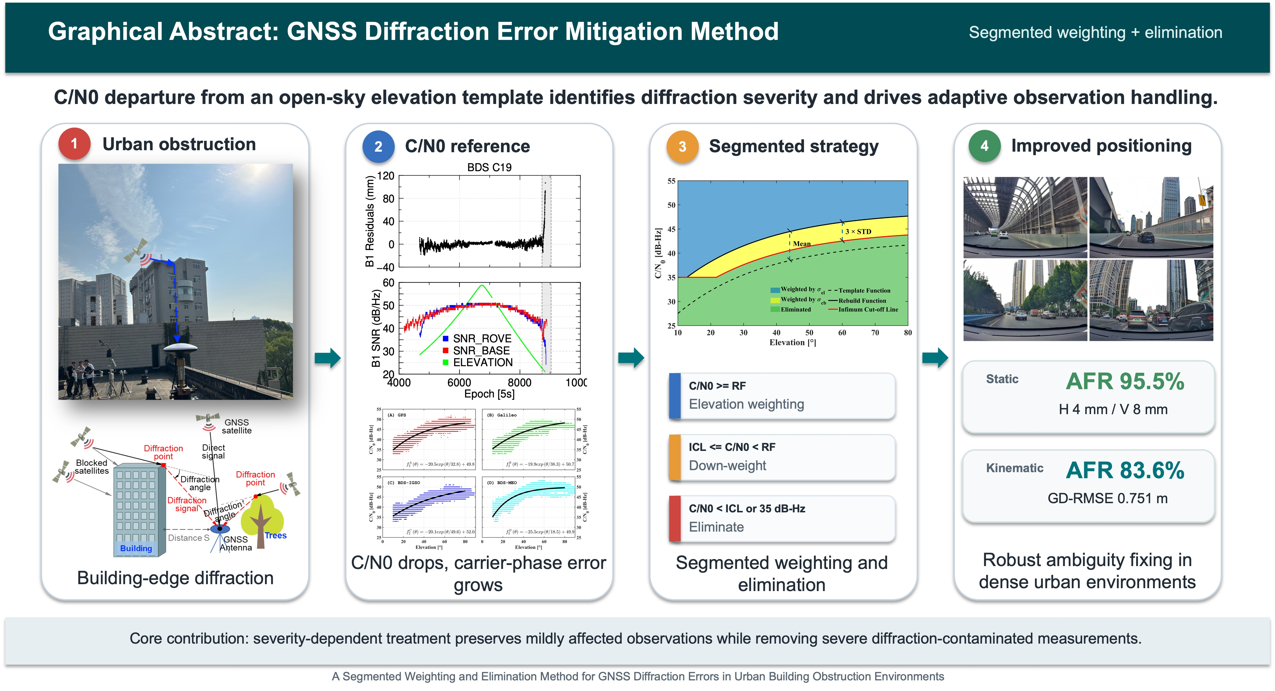
Graphical Abstract

1. Introduction

Global Navigation Satellite Systems (GNSSs) have become an indispensable spatial information infrastructure in modern society, providing fundamental positioning, navigation, and timing services for a wide range of fields such as surveying and mapping, transportation, autonomous driving, and the Internet of Things. With the accelerating pace of urbanization, urban spaces are increasingly characterized by dense buildings, towering skyscrapers, and narrow streets. In such conditions, GNSS signal propagation suffers severe interference: line-of-sight (LOS) signals are heavily obstructed, significantly reducing the number of visible satellites; multipath effects become pronounced [1,2]; and non-line-of-sight (NLOS) signal reception is common [3], introducing substantial measurement errors. These factors collectively lead to a sharp decline in the accuracy, availability, and reliability of traditional GNSS positioning in densely built urban areas [4,5,6], making it difficult to meet the demanding requirements for centimeter-level or even millimeter-level precise positioning. Therefore, researching how to achieve stable, reliable, and high-precision GNSS positioning in densely constructed urban environments has become a critical technical bottleneck for enabling cutting-edge applications such as smart cities, autonomous vehicles, intelligent construction, and deformation monitoring, carrying both significant theoretical importance and urgent practical needs.
The integrated processing of Global Navigation Satellite Systems (GNSSs), including GPS, BDS, Galileo, and GLONASS, can effectively alleviate the issue of insufficient numbers of visible satellites in complex, highly obstructed environments. Efforts have also been made in the fields of hardware design, signal processing, and data processing to mitigate multipath effects [7,8,9]. Numerous multipath mitigation techniques have been proposed and are now widely employed in navigation, deformation monitoring, and other high-precision positioning applications [10,11].
In recent years, increasing attention has been devoted to non-line-of-sight (NLOS) errors. An NLOS error refers to the error that occurs when a GNSS antenna receives a reflected or diffracted signal in an obstructed environment. Compared with the direct path of a satellite signal in unobstructed conditions, the propagation path of an NLOS signal is longer, which can introduce significant ranging errors and degrade GNSS positioning accuracy. Currently, NLOS signal reception is commonly identified using external sources such as fisheye cameras [12], Light Detection and Ranging (LiDAR) scanning [13,14], 3D Mapping Aided (3DMA) [15,16], or antenna array techniques [17]. Following identification, down-weighting or elimination strategies are typically applied to mitigate NLOS-induced errors. In sensor-independent approaches, Han et al. (2020), Xi et al. (2023), and Ren et al. (2023) proposed identifying obstruction edges based on C/N0 measurements or a posteriori residuals, and developed an azimuth-dependent cut-off elevation method, which has been successfully applied in static positioning scenarios [18,19,20,21]. Moreover, data-driven methods, such as Convolutional Neural Networks (CNNs) [22], Long Short-Term Memory networks (LSTM) [23], decision trees [24], support vector machines (SVMs) [25,26], and deep reinforcement learning (DRL) [27], have been widely adopted for NLOS signal detection. These methods leverage the powerful nonlinear approximation capabilities of machine learning models to capture hidden patterns in environmental and observational data, enabling accurate classification of signal types (LOS and NLOS) and correction of NLOS biases, thereby improving GNSS positioning accuracy in complex urban environments [28].
In dense urban environments, a substantial portion of NLOS error arises from diffraction at building edges. Diffraction refers to the bending of the signal path around an obstruction edge, allowing the receiver to track the signal within the shadow region [29,30,31]. Previous studies have shown that diffraction error can exceed one carrier wavelength [18,32], far beyond the theoretical upper bound of the multipath, namely one quarter of the carrier wavelength [33,34]. It is therefore an important cause of cycle slips, precision degradation, and reduced solution reliability. At the same time, the temporal behavior of diffraction error depends on the geometry of the surrounding obstruction, which is often complex and site-specific, making universal correction difficult [18].
Our previous work derived a theoretical model for diffraction error from the geometric configuration of the satellite–building–antenna signal path, and diffraction errors extracted from data collected in building-obstructed environments were shown to be consistent with that model. These results indicate that diffraction error exhibits a clear temporal trend, increasing or decreasing monotonically from the millimeter level to as much as 0.2 m [21]. Such diffraction typically occurs near building edges. However, existing NLOS detection methods often do not account for the gradual development of diffraction error and instead directly down-weight or exclude observations without evaluating the actual error magnitude. In high-precision positioning applications in dense urban environments, this can lead either to errors that far exceed the assumed stochastic model or to the unnecessary rejection of only slightly affected observations. Effective detection, assessment, and mitigation of diffraction errors are therefore essential for reliable and accurate positioning in obstructed environments. In this study, we further demonstrate the correlation between diffraction error and C/N0 and propose a strategy that down-weights moderately affected observations while removing severely diffraction-contaminated ones. Compared with conventional approaches, the proposed method provides a more rational assessment of error severity and applies adaptive processing accordingly, thereby improving positioning robustness and accuracy. The key contribution of this study is therefore not a generic C/N0 reweighting scheme, but a severity-dependent segmented treatment that preserves slightly affected observations, down-weights moderately contaminated observations, and removes severely diffraction-affected observations.

2. Diffraction Effects

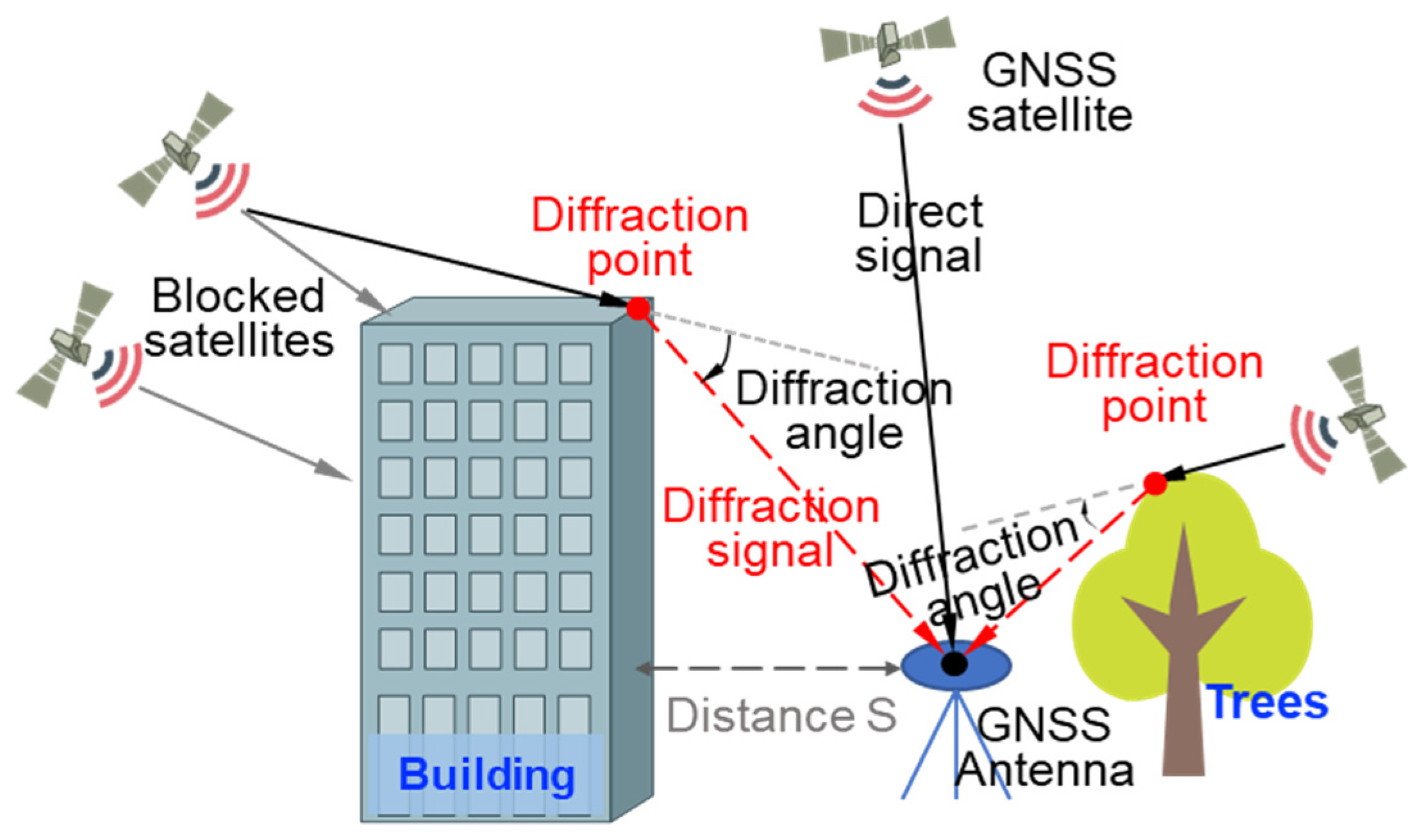
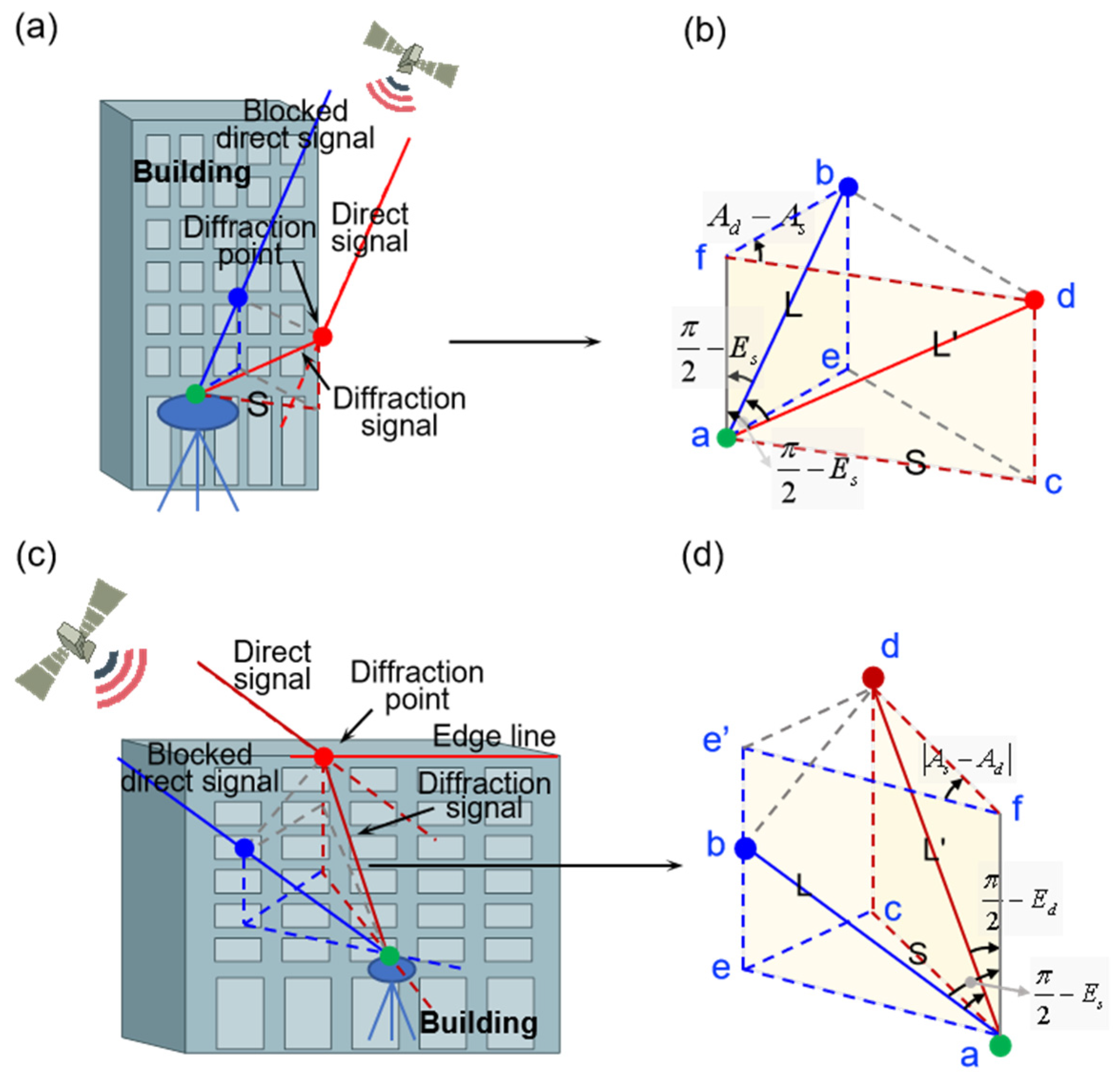
Diffraction refers to the phenomenon in which a satellite signal bends around the edges of obstacles such as buildings, trees, and terrain slopes, thereby enabling reception within the shadow region where the line of sight is blocked, as illustrated in Figure 1. Unlike the direct signal path in unobstructed conditions, a diffracted signal travels an additional distance before reaching the receiver. This excess path length is defined here as the GNSS diffraction error. Based on the satellite–obstruction–antenna geometry shown in Figure 2, the horizontal and vertical components of the diffraction error can be modeled by Equations (1) and (2), respectively. In the equations, E s and A s indicate the elevation and azimuth of the satellites, and E d and A d are the elevation and azimuth of the diffraction point compared to the location of the GNSS antenna. S denotes the distance of the GNSS antenna to the obstruction. Detailed derivations are provided in Xi et al. (2025) [21].
d H = L L = S cos E s 1 sin 2 E s + cos 2 E s × cos A d A s
d V = L L = S cos E d 1 sin E s × sin E d + cos E s × cos E d × cos A d A s
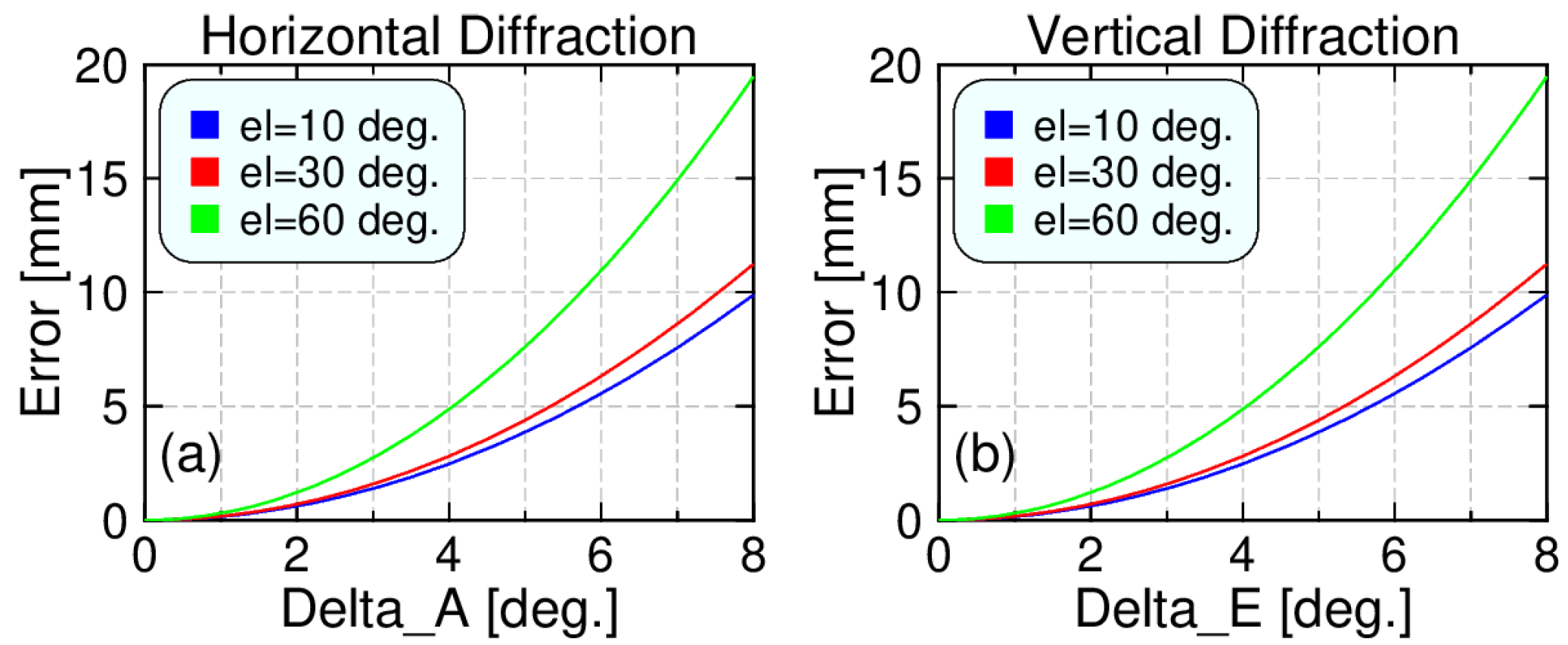
According to these equations, the magnitude and temporal evolution of the diffraction error depend on the relevant diffraction geometry. Figure 3 illustrates the diffraction error as a function of diffraction angle and obstruction distance when the antenna-to-obstruction distance is 1 m. The error increases rapidly as the diffraction angle increases, and its amplitude scales accordingly with the geometric configuration.
In Equations (1) and (2), the horizontal and vertical diffraction error components are controlled by the satellite elevation and azimuth, the elevation and azimuth of the diffraction point with respect to the antenna, and the antenna-to-obstruction distance S in Figure 2.
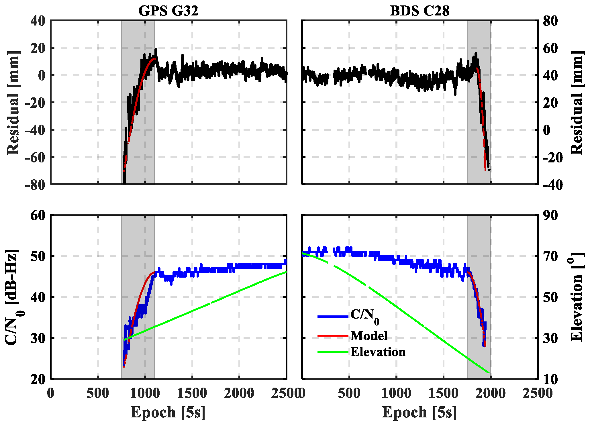
Figure 4 presents carrier-phase residual time series for satellites G32 and C28, extracted using a differential phase-based kinematic post-processing method [35], together with the corresponding C/N0 and elevation time series. The residuals within the shadowed interval exhibit a clear monotonic trend, consistent with the theoretically predicted evolution of diffraction error. At the same time, a distinct drop in C/N0 is observed for both satellites, matching the expected behavior of diffraction error as a function of diffraction angle. Because diffraction is a form of NLOS propagation, the magnitude of the C/N0 degradation is also related to diffraction angle. The C/N0 time series for diffraction-affected observations can therefore be modeled using Equations (3) and (4).
C / N 0 H = K cos E s 1 sin 2 E s + cos 2 E s × cos A d A s
C / N 0 V = K cos E d 1 sin E s × sin E d + cos E s × cos E d × cos A d A s
where K is a constant distinct from S in Equations (1) and (2). In Figure 4, the diffraction errors are modeled using Equations (1) and (2), while the corresponding C/N0 time series are modeled using Equations (3) and (4).
The models defined by Equations (1)–(4) characterize both diffraction error and the corresponding C/N0 time series well. Diffraction error and C/N0 therefore share a similar temporal behavior, indicating that C/N0 can be used as an effective indicator of diffraction occurrence.
As indicated by the preceding analysis, conventional elevation-dependent weighting methods are not well suited to observations affected by diffraction. As shown in Figure 4, diffraction error may accumulate to a level that exceeds the assumptions embedded in standard stochastic models. Moreover, traditional C/N0-based weighting methods do not always down-weight these observations appropriately, because the C/N0 value does not necessarily reflect the true magnitude of the diffraction error. In such cases, severely distorted observations should be excluded rather than merely down-weighted. For this reason, the present study proposes a segmented weighting and elimination strategy that detects diffraction-affected signals and applies adaptive down-weighting or removal according to error severity.

3. Methods

Under open-sky conditions, the elevation–C/N0 time series for each satellite generally exhibits a positive correlation; that is, C/N0 increases as satellite elevation increases. When diffraction occurs, however, this correlation is disrupted, and C/N0 may decrease markedly as diffraction angle increases. At the same time, the diffraction error may increase or decrease sharply [18].

3.1. Standardized Template Function Model of “Elevation–C/N0”

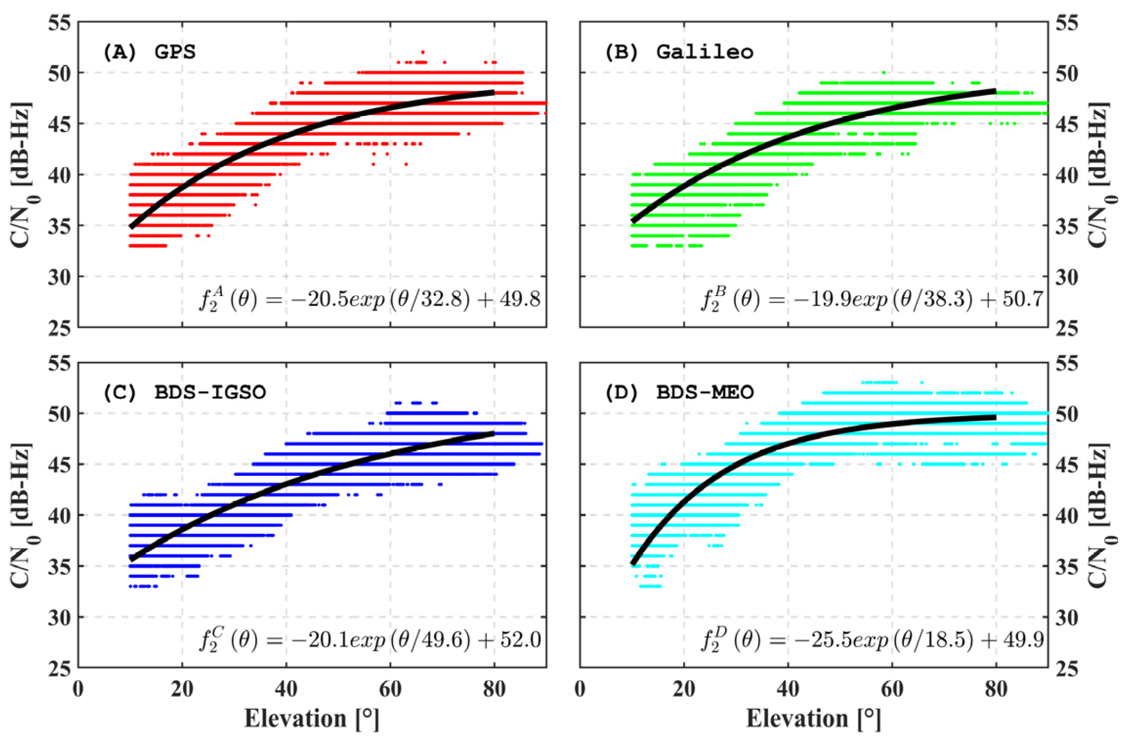
In the present study, the open-sky template is fitted separately for each constellation/orbit class (GPS, Galileo, BDS-IGSO, and BDS-MEO) using pooled open-sky data. During implementation, each satellite observation is compared with the template of its corresponding class at the same elevation. Therefore, Figure 5 is presented at the system/orbit-class level, whereas the following figures could show satellite-specific trajectories.
Based on the correlation between diffraction error and C/N0, a standardized elevation–C/N0 template function is established for each GNSS class using data collected under open-sky conditions. A segmented weighting and elimination strategy is then constructed by comparing C/N0 measurements obtained in obstructed environments with the corresponding values predicted by the standardized template.
(1)
“Elevation–C/N0” correlation model fitting with a least-squares method
In this study, an exponential function is used to model the elevation–C/N0 relationship under open-sky conditions, as shown in Equation (5).
f ( θ ) = a 0 exp θ / a 1 + a 2
where θ indicates the elevation and f ( θ ) is the corresponding C/N0. The estimated parameters are
x = a 0 a 1 a 2 T
Under open-sky conditions, the C/N0 samples within each satellite elevation interval are represented as a column vector y, and f denotes the fitting function for that elevation interval. The least-squares problem can then be written as
min a , b , c y f 2 2 = min a , b , c i = 1 n y i a 0 exp ( θ i / a 1 ) a 2 2
where n is the number of samples and · 2 denotes the norm of a column vector. Since the formula is nonlinear, we use the Gauss–Newton method to solve it iteratively.
If we define the prior residuals as
e i = y i a 0 exp ( θ i / a 1 ) a 2
then, the partial derivative of the parameter to be estimated could be
J = f a 0 f a 1 f a 2
where J is the Jacobian Matrix in n × 3. According to the increment equation of the Gauss–Newton method, the increment in the estimated parameters Δ x could be
Δ x = ( J T J ) 1 J T e
where e is the column vector of the prior residual. Therefore, the updated parameters are
x = x + Δ x
This procedure is repeated iteratively until the parameter increment falls below the prescribed threshold, yielding the basic template function
x f i r s t = a 0 a 1 a 2 T f 1 G ( θ ) = a 0 exp θ / a 1 + a 2
Because the number of C/N0 measurements differs across elevation intervals and outliers may be present, a weighted least-squares approach is used to fit the model in Equation (12). The observation weight is defined as
ω i k = N k , k + 1 C i f 1 ( θ C i )
where ω i k is the weight of the i-th C/N0 measurement in the k-th elevation interval, f 1 θ C i is the fitted value in Equation (12), and N k , k + 1 is the number of samples in the k-th elevation interval. Equation (13) indicates that observations in densely sampled intervals and those closer to the fitted value receive higher weights. The weight matrix W is therefore
W = ω 1 ω 2 ω n
and the solution of the weighted least-square is
Δ x = ( J T W J ) 1 J T W e
The parameters estimated from the second fit then yield the final template function, where G denotes the satellite system or orbit class.
x second = a 0 a 1 a 2 T f 2 G ( θ ) = a 0 exp θ / a 1 + a 2
Figure 5 shows the fitted elevation–C/N0 model. The fit closely follows the overall trend of C/N0 variation with elevation. We further discretize the model and take the median value within 1-degree elevation bins from 10 degrees to 80 degrees to obtain the template vector
C G f i t = f 2 G ( 10.5 ) f 2 G ( 11.5 ) f 2 G ( 2 k + 1 2 ) f 2 G ( 79.5 ) T
where C G f i t is the template vector of the C/N0.
(2)
Difference statistics of the observed and the model value
For each satellite, the C/N0 measurements within each 1-degree elevation bin are averaged as
C k , k + 1 G , p r n i = j = 1 N k , k + 1 C j N k , k + 1 , k = ( 10 , 11 , , 79 )
where C k , k + 1 G , p r n i is the mean C/N0 value within the elevation interval [k, k + 1]. The averaged C/N0 time series from 10 degrees to 80 degrees can therefore be written as
C G p r n i = C 10 , 11 G , p r n i C 11 , 12 G , p r n i C k , k + 1 G , p r n i C 79 , 80 G , p r n i T
The difference vector between the observed C G p r n i and modeled values C G f i t is then given by d G , and the mean and corresponding standard deviation (STD) of d G can be computed as
x G p r n i ¯ = 1 70 d G 1 , σ G p r n i = 1 69 d G x G p r n i ¯ 2
where · 1 is the 1-norm of vector, and
d G = C G p r n i C G f i t , x G p r n i ¯ = x G p r n i ¯ x G p r n i ¯ x G p r n i ¯ T
(3)
Template “elevation–C/N0” model reconstruction in an open environment
The first step is to assess whether the C/N0 time series for a given satellite is suitable for template reconstruction. If it exceeds the threshold σ t h r e s , the time series is considered too variable for reliable modeling. Assuming that C/N0 fluctuations follow a normal distribution, 99.7% of the data should lie within three standard deviations. We therefore apply a three-sigma rule to exclude outliers, and the reconstruction model is defined as follows:
C max G , p r n i ( θ ) = f 2 G ( θ ) + x G p r n i ¯ + 3 σ G p r n i C min G , p r n i ( θ ) = f 2 G ( θ ) + x G p r n i ¯ 3 σ G p r n i
where C max G , p r n i θ and C min G , p r n i θ are the upper and lower bounds of the reconstruction model, and the threshold value is set to 1.7 in this study. The screening threshold τ = 1.7 was selected empirically from the open-sky calibration dataset so that stable arcs are retained while strongly fluctuating arcs are excluded from template reconstruction.

3.2. Segmented Weighting and Elimination Method

Previous studies have shown that diffraction error typically increases or decreases approximately linearly, with its magnitude depending on diffraction angle and distance to the obstructing edge [18,21]. This indicates that diffraction error evolves gradually as the signal geometry changes. Accordingly, we propose a strategy that down-weights observations affected by small to moderate errors and excludes those affected by large errors. The error magnitude is assessed using the elevation–C/N0 reference model described above. The resulting adaptive weighting and elimination scheme can be expressed as follows:
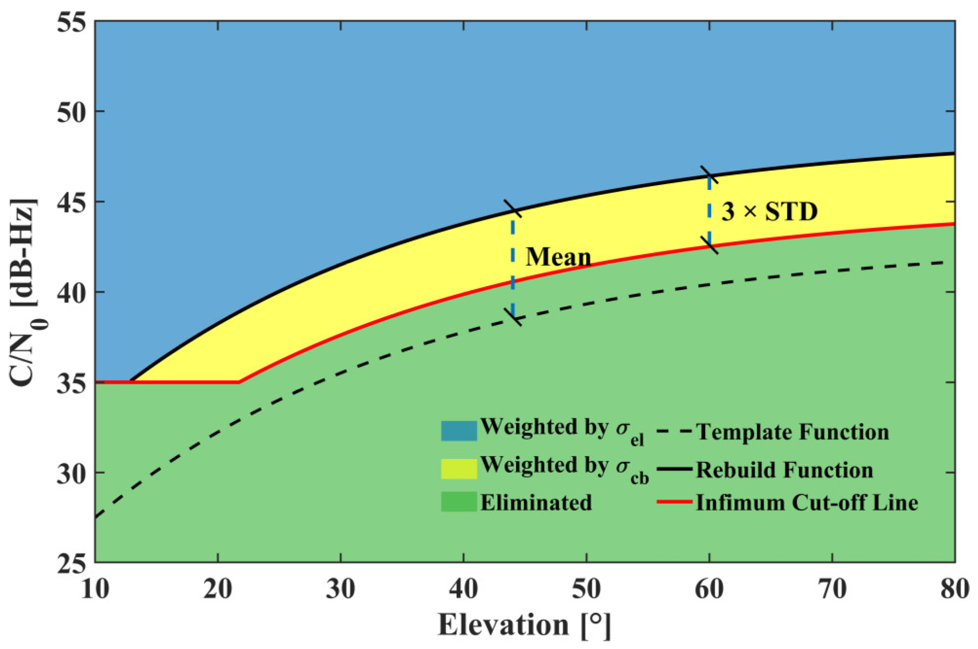
w = 0 , ( C / N 0 < C min G , p r n i ) ( C / N 0 < 35 dB / Hz ) 1 / σ e l 2 , C / N 0 > f 2 G ( θ ) 1 / σ c b 2 , f 2 G ( θ ) C / N 0 C min G , p r n i ( θ )
where C / N 0 is the observed C/N0, w is the weight assigned to the carrier-phase observation, and σ c b 2 is the variance of an observation contaminated by diffraction but still considered suitable for down-weighting; in this study, such errors are typically smaller than 50 mm. σ c b 2 is the variance determined jointly by the elevation-dependent model and the C/N0-based model, as defined in Equation (24).
σ c b 2 = σ e l 2 + σ G p r n i σ G m σ s n r 2
where σ G m is the mean value of σ G p r n i .
According to Equation (23), when the observed C/N0 is greater than or equal to the template value at a given elevation, the carrier-phase observation is considered good-quality and the conventional elevation-dependent weighting model is applied. When the observed C/N0 lies between the template value and the lower bound of the reconstructed C/N0 model, σ c b 2 is used to determine the weight. When the observed C/N0 falls below the lower bound, the corresponding observation is excluded. In addition, based on the open-sky C/N0 distribution, observations with C/N0 below 35 dB-Hz are also excluded, although this threshold may vary across receiver types. The complete weighting and elimination procedure is illustrated in Figure 6.
For software or firmware implementation, the modeled C/N0 template is queried at each epoch using the instantaneous satellite elevation. The observed C/N0 is then compared with the Reconstruction Function (RF) and the Infimum Cut-off Line (ICL) to determine one of three actions: conventional elevation-based weighting, combined elevation- and C/N0-based down-weighting, or direct observation exclusion. The proposed method can therefore be implemented in the stochastic model or pre-screening module of RTK/PPP processing software without changing the basic observation equations.
In this study, the 35 dB-Hz cut-off is used as an empirical lower bound for stable carrier tracking with the K803-based receiver and geodetic antennas. The 5 dB-Hz differential threshold was selected as a conservative short-baseline rejection criterion, and the ambiguity ratio threshold of 2.2 was adopted to balance fix availability and reliability in the obstructed urban datasets. These empirical thresholds may need to be recalibrated for different receivers, antennas, firmware versions, or urban environments.

4. Experiments and Results

This section first presents the experimental data and processing setup, and then open-sky template characterization, and finally the static and kinematic positioning results obtained with the four processing strategies.

4.1. Experimental Data and Processing Setup

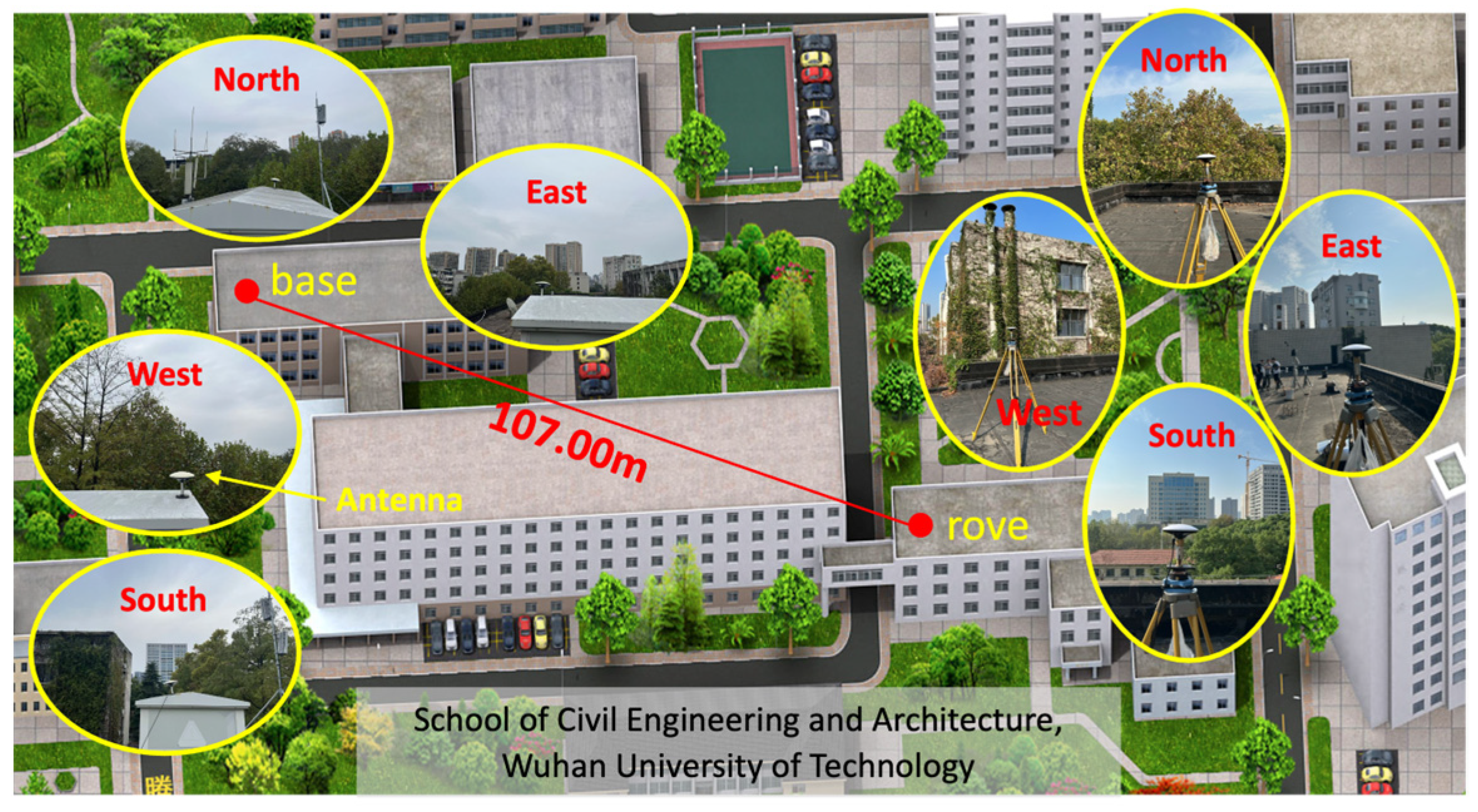
The open-sky calibration data used to build the templates were collected on the rooftop platform shown in Figure 7 using two K803-based multi-frequency GNSS receivers and geodetic antennas. The calibration baseline was 107.00 m long. The static urban experiment was conducted on 18 September 2023 from 17:00 to 24:00 UTC with a sampling interval of 5 s, during which the rover remained stationary for approximately 9 h under severe building obstruction. The vehicle-based kinematic experiment used the same receiver–antenna configuration, with two antennas mounted on the roof and a sampling rate of 1 Hz.
The data-processing platform was an RTKLIB (2.4.3 b34)-based in-house post-processing program in which the proposed weighting and elimination rule was implemented in the stochastic modeling stage. The millimeter-level values reported for the static test correspond to ambiguity-fixed relative positioning on short baselines with geodetic antennas and quality-controlled carrier-phase observations; they should not be interpreted as standalone consumer-grade urban positioning accuracy. The K803 board is a compact multi-frequency OEM receiver module rather than a smartphone-grade single-frequency device.
Accordingly, the following section focuses on the characteristics of the open-sky templates and the resulting positioning performance, while the main acquisition and processing settings are summarized here and in Table 1.

4.2. Open-Sky Template Characterization

Using the open-sky dataset summarized in Section 4.1, Figure 7 shows the experimental platform and surrounding observing conditions for the reference station (BASE) and rover station (ROVE). Both stations tracked GPS, Galileo, BDS-2, and BDS-3 satellites, and the resulting data were used to construct the open-sky elevation–C/N0 reference templates.
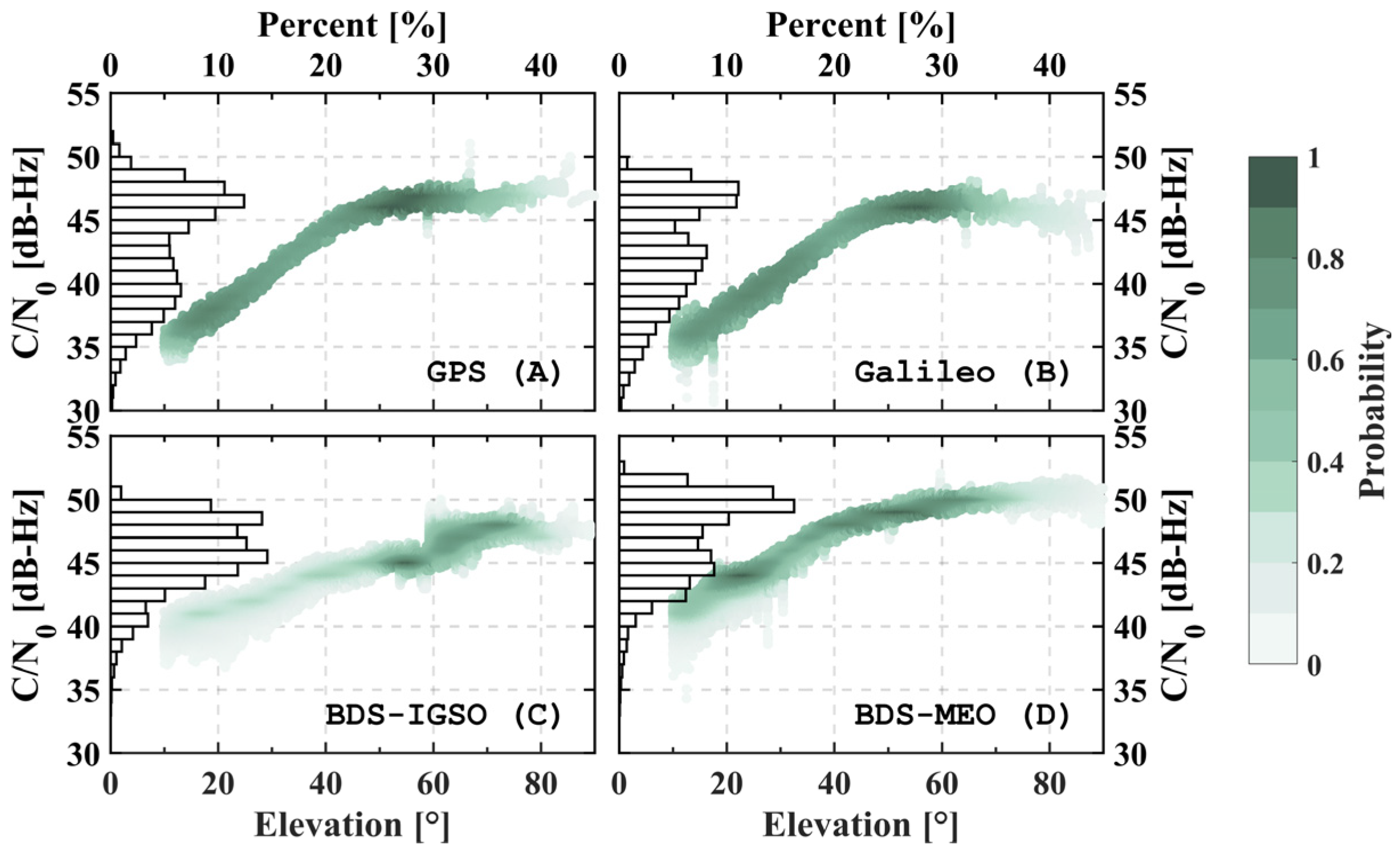
Figure 8 presents the probability density distributions and frequency histograms of the C/N0 time series for GPS, Galileo, BDS-IGSO, and BDS-MEO satellites. Although the overall elevation–C/N0 trend is similar across the four satellite classes, their probability density distributions differ markedly. The C/N0 distributions of GPS and Galileo are broadly similar and both exhibit a bimodal pattern, although the second peak for Galileo is about 3 dB-Hz higher than that for GPS. For BDS satellites, the C/N0 values of IGSO satellites are concentrated mainly around 45 dB-Hz, whereas BDS MEO satellites generally exhibit higher C/N0 values than the other constellations, with a peak near 50 dB-Hz. These results indicate that, despite a similar elevation-dependent trend, the elevation–C/N0 relationship varies across satellite systems, and both the data density within each elevation interval and the occurrence of anomalous values differ substantially. The subsequent experiments therefore establish the standardized elevation–C/N0 template separately for each satellite class to ensure system-specific accuracy and robustness.

4.3. Static Positioning Experiment

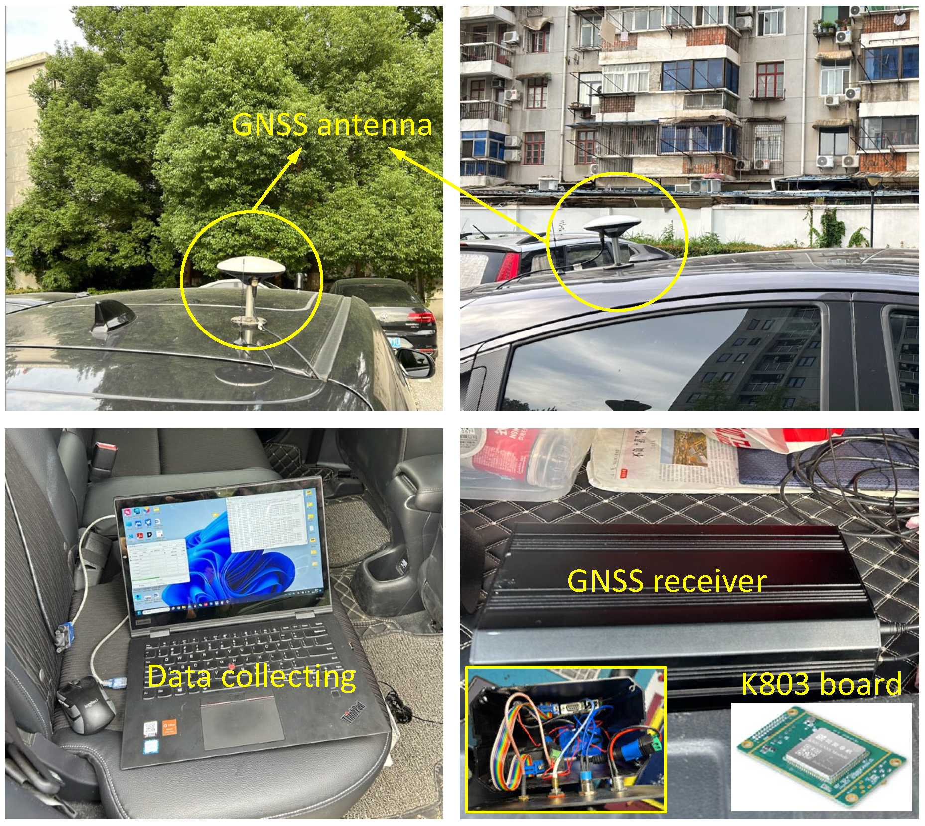
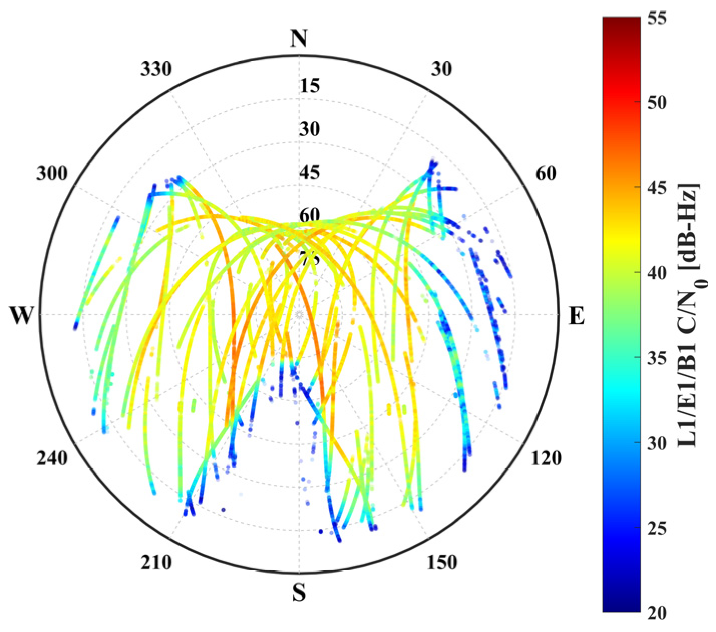
To evaluate the performance of the proposed method, the open-sky data collected from the platform shown in Figure 7 were first used to establish the elevation–C/N0 reference model and determine the weighting and elimination strategy defined in Equation (23). The rover receiver and antenna were then mounted on the roof of a vehicle and kept stationary for approximately 9 h in a severely obstructed urban environment to simulate a static positioning scenario. Data were collected on 18 September 2023 from 17:00 to 24:00 UTC. The rover receiver was a custom-developed unit based on the K803 GNSS module manufactured by ComNav Technology Ltd., Shanghai, China, configured to track GPS, BDS, and Galileo satellites at a 5 s sampling interval. Figure 9 shows the rover setup and its surrounding environment, while Figure 10 presents the corresponding C/N0 sky plot. These figures indicate substantial signal obstruction from both trees and buildings, particularly a tall building to the south of the station. The base station was the same as that shown in Figure 7, and the baseline length was approximately 1 km.
Single-epoch processing was used to evaluate the ambiguity-fixing rate (AFR) and positioning accuracy. The detailed processing strategy is summarized in Table 1.
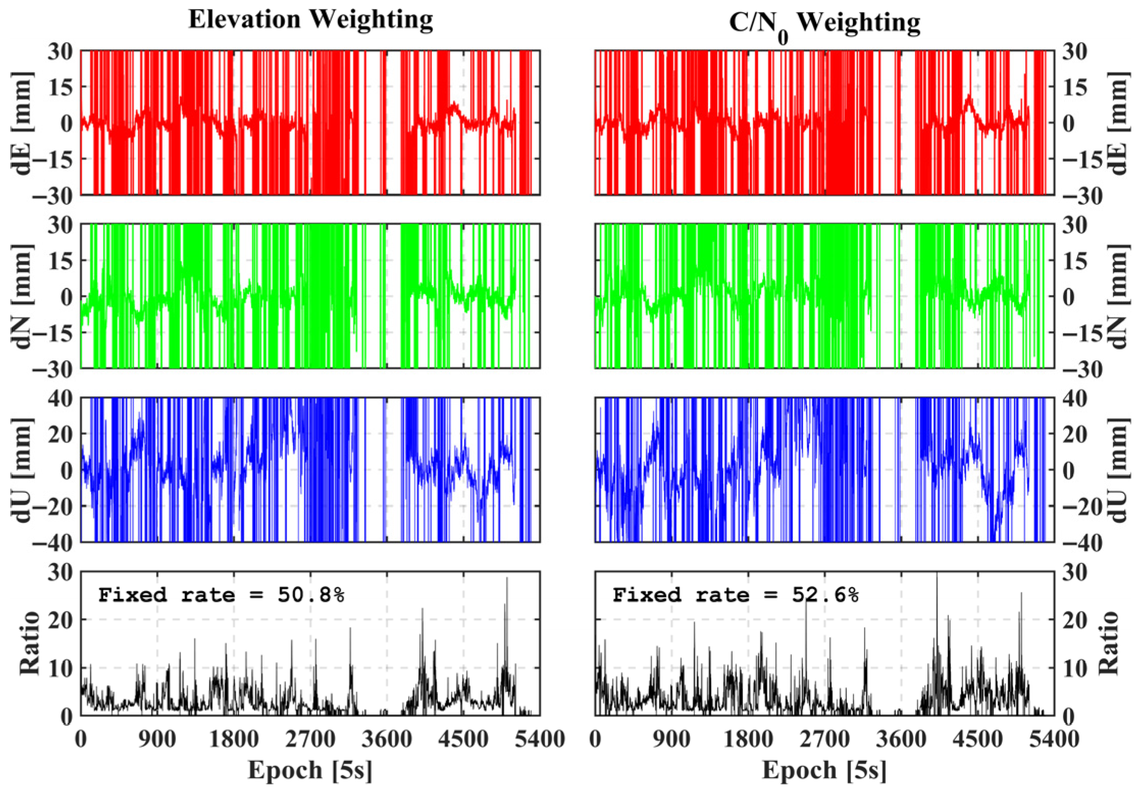
We first processed the data using the conventional elevation-based and C/N0-based weighting methods listed in Table 1, as shown in Figure 11. Under severe obstruction, the AFR achieved by the elevation-based and C/N0-based weighting methods was only 50.8% and 52.6%, respectively. The data gap around epoch 3600 is attributed to large errors in the pseudorange or carrier-phase measurements. These results indicate that conventional weighting methods do not adequately account for diffraction-affected observations and therefore yield suboptimal positioning performance.
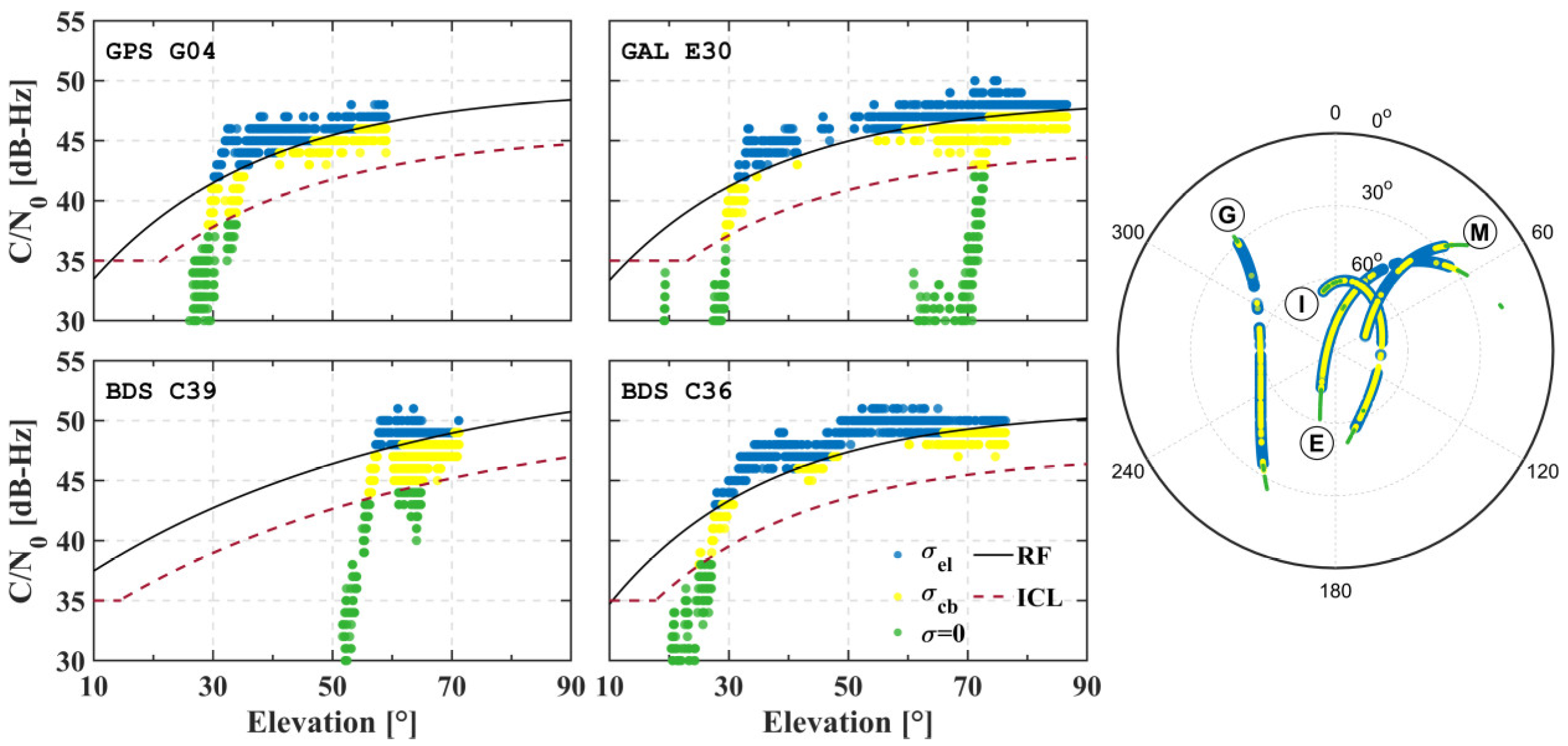
To illustrate the segmented treatment of diffraction error, we selected the C/N0 and elevation-angle series for GPS-G04, GAL-E30, BDS-C39, and BDS-C36, as shown in Figure 12. The black solid lines represent the Reconstruction Function (RF), and the dark red dashed lines represent the Infimum Cut-off Line (ICL), which define the thresholds for down-weighting and exclusion, respectively. When the observed C/N0 is higher than the RF at a given elevation, the conventional elevation-based weighting method is applied. When the observed C/N0 lies between the RF and ICL, a combined elevation- and C/N0-based weighting strategy is used. Observations with C/N0 values below the ICL are excluded during processing. Because signal characteristics differ among satellites, the RF and ICL models may vary from one satellite to another. Here, the RF and ICL curves are obtained by projecting the corresponding class-level open-sky template onto the actual elevation trajectory of each selected satellite.
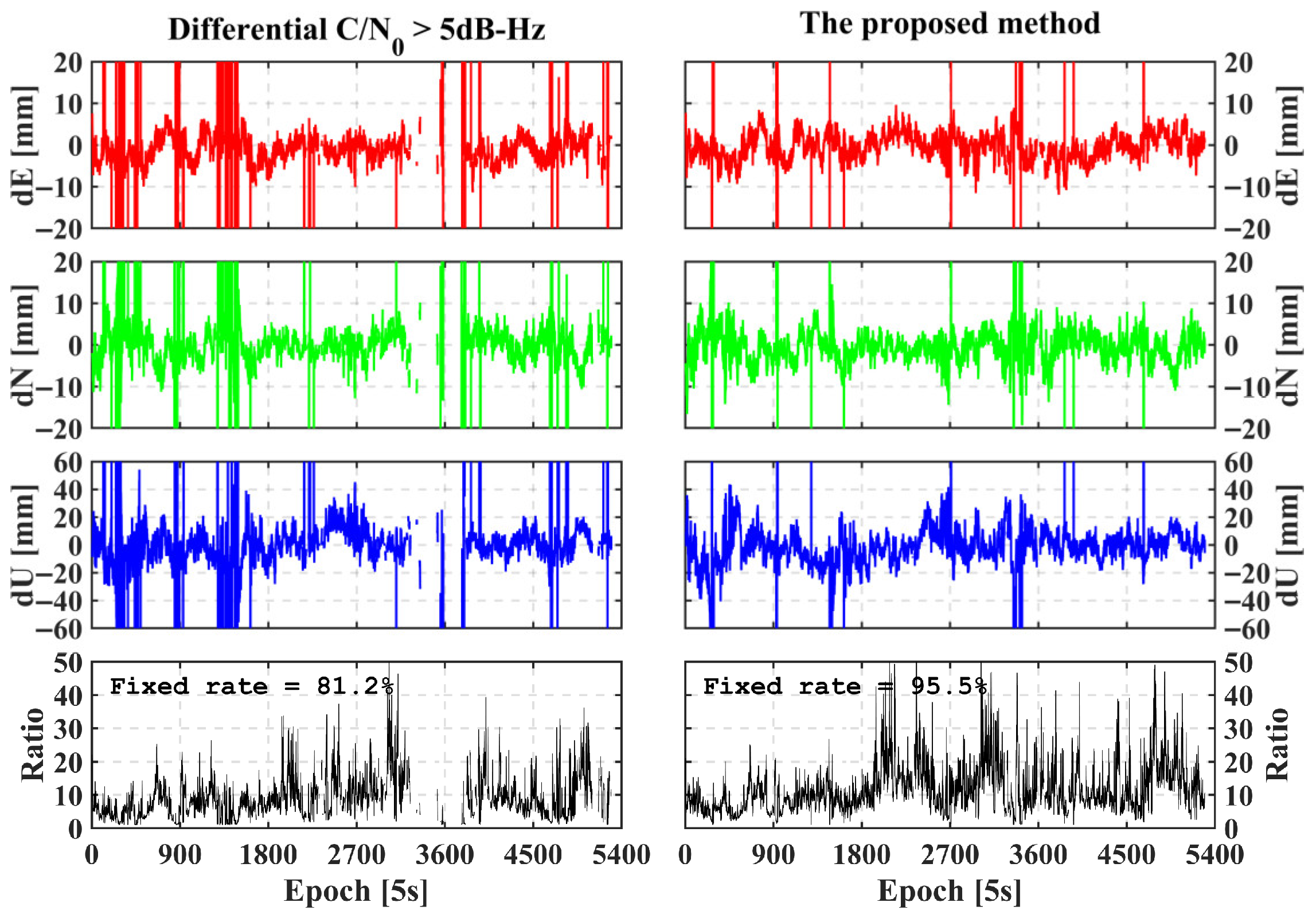
To further evaluate the ability of the proposed method to mitigate diffraction error, we processed the data using both the proposed strategy and a differential C/N0 method (Han et al., 2025) [38]. The differential C/N0 method computes the C/N0 difference between the reference and rover stations. Because diffraction is unlikely to occur simultaneously at both stations on a short baseline, this differential signal can be compared with a predefined threshold. If the difference exceeds that threshold, the corresponding rover observation is excluded. This strategy is physically reasonable because diffraction-affected signals often exhibit a pronounced loss of C/N0, as also shown in Figure 4.
Figure 13 presents the positioning results obtained with these two methods, using a differential C/N0 threshold of 5 dB-Hz. Relative to the conventional elevation-based and C/N0-based weighting strategies shown in Figure 11, the differential C/N0 method increases the AFR to more than 80%. This indicates that large diffraction errors are better handled by exclusion than by simple down-weighting. With the proposed segmented weighting and elimination strategy, the AFR further improves to 95.5%, and the data gap around epoch 3600 is effectively removed. We then extracted all fixed solutions from the four processing schemes and assessed their consistency using Spearman’s rank correlation coefficient. The average correlation coefficient across the three coordinate components reached 0.75, indicating high internal consistency and supporting the reliability of the estimated solutions.
Table 2 summarizes the detailed positioning statistics. The average ambiguity–search ratio for both the differential C/N0 method and the proposed method is substantially higher than that of the conventional weighting strategies. The proposed method achieves the highest search ratio, 11.85, and also provides a higher data-integrity index than the other approaches. The average number of tracked satellites and the PDOP values for the differential C/N0 and proposed methods are slightly degraded relative to the weighting-based strategies, reflecting the selective exclusion of low-quality observations. Once ambiguities are correctly fixed, all methods deliver broadly comparable coordinate accuracy. Nevertheless, the proposed method yields slightly better positioning performance than the differential C/N0 method, especially in terms of continuity and robustness under severe obstruction.
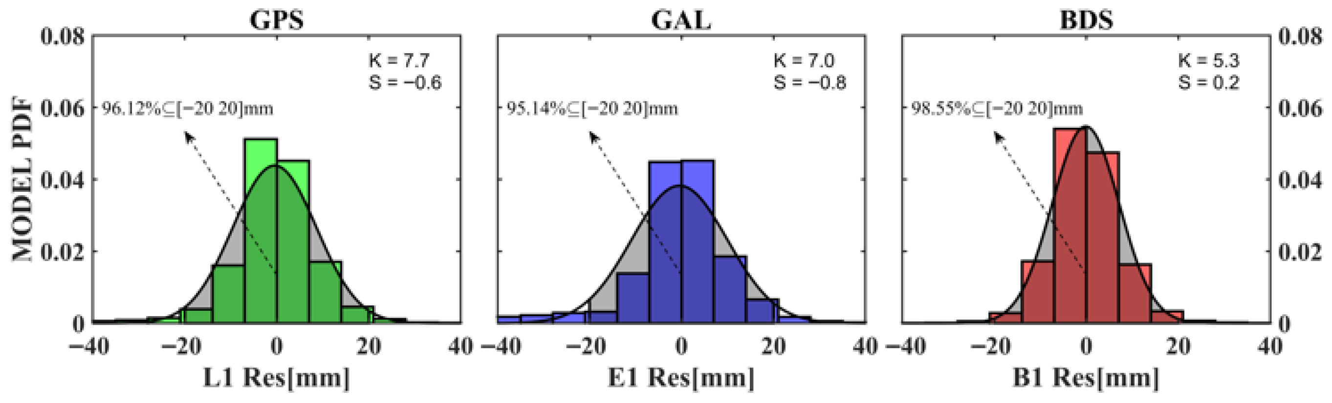
Figure 14 shows the histograms of the a posteriori residuals for GPS, Galileo, and BDS. For each satellite system, the absolute values of kurtosis and skewness are below 10 and 3, respectively, indicating that the residual distributions are approximately symmetric and moderately peaked and therefore close to normal. Moreover, more than 95% of the residuals fall within ±2 cm, demonstrating that large diffraction errors are effectively mitigated by the proposed method.

4.4. Kinematic Positioning Experiment

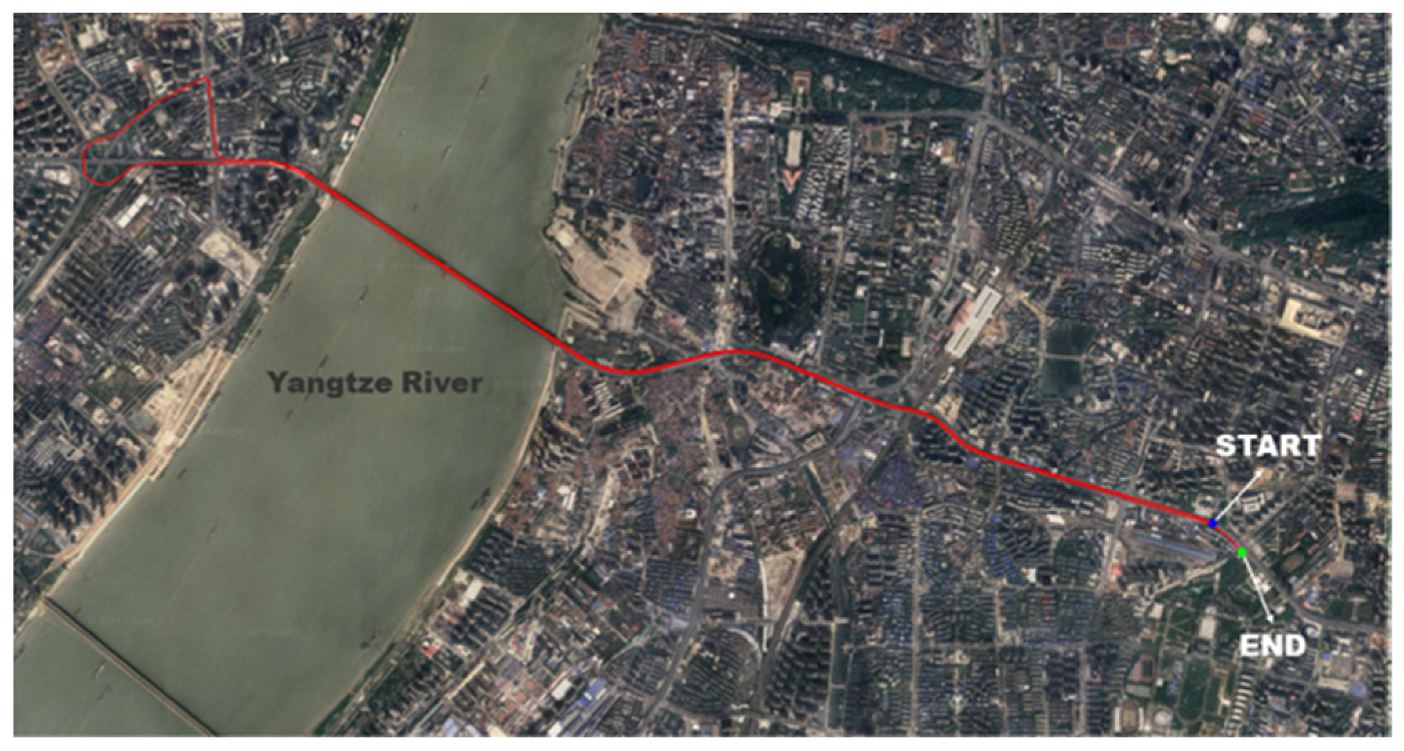
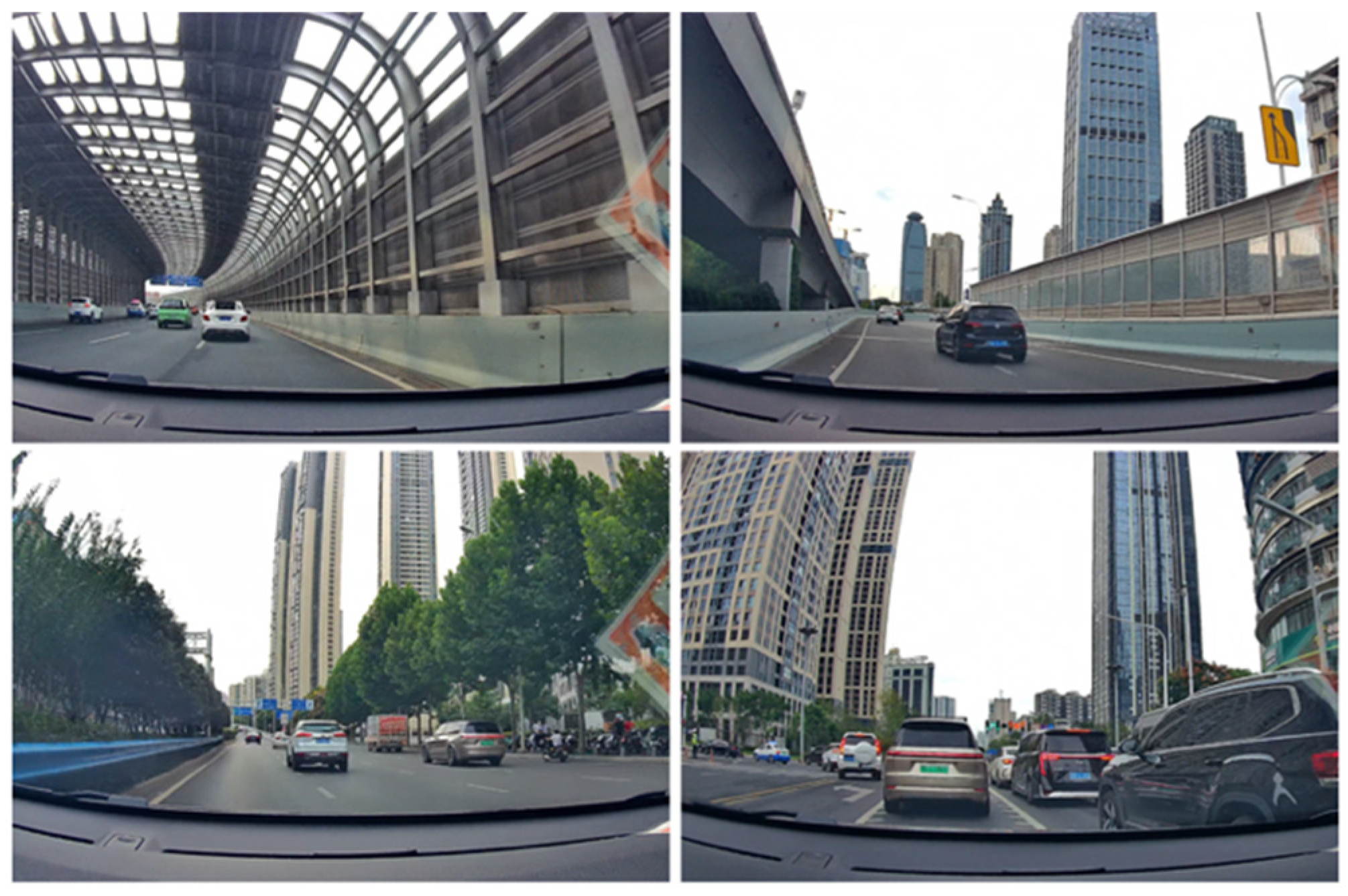
To further assess the performance of the proposed method in kinematic positioning, a vehicle-based field experiment was conducted. Vehicles typically travel through commercial and residential areas characterized by substantial building obstruction. Figure 15 shows the test route, and Figure 16 presents representative examples of the complex obstructed environments encountered during the experiment. The hardware configuration was the same as that shown in Figure 9. In this experiment, however, two antennas were mounted on the roof of the vehicle and connected to two K803 GNSS receivers for independent positioning and cross-validation. The GNSS data were collected at a sampling rate of 1 Hz.
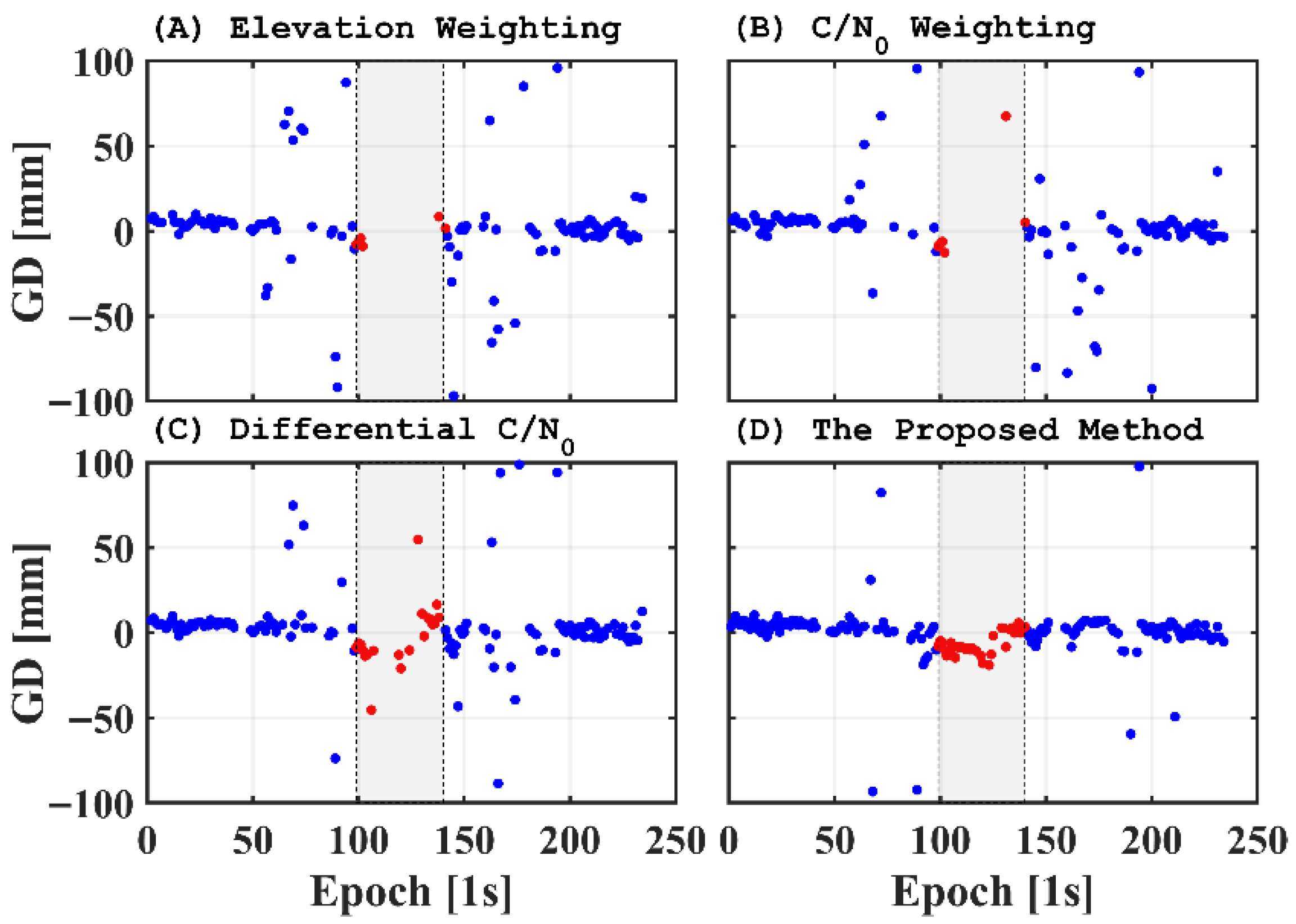
All four methods were then applied to process the kinematic dataset. Because the baseline length between the two GNSS antennas is precisely known, the geometric distance (GD) was computed and used as the reference for performance evaluation. Positioning accuracy was assessed from the residuals defined by
G D j i = ( X j x j i ) 2 + ( Y j y j i ) 2 + ( Z j z j i ) 2 G D T r u e
where G D T r u e is the true distance between the two antennas; X j , Y j , Z j and x j , y j , z j are the coordinates of the first and second antennas, respectively; and GD denotes the difference between the measured and true values. The AFR and positioning-accuracy statistics are listed in Table 3.
Here, X , Y , Z and x , y , z denote the Earth-Centered Earth-Fixed (ECEF) coordinates of the two antenna phase centers estimated independently at each epoch.
The results show that the AFR is only about 40% for the elevation-based and C/N0-based weighting methods. Both weighting strategies also exhibit substantial data gaps, particularly within the shaded interval in Figure 17, which corresponds to the vehicle passing through a dense urban intersection surrounded by tall buildings. For the differential C/N0 method, the AFR improves to 65.8%, and data integrity improves accordingly. By contrast, the proposed method achieves an AFR of 83.6% and yields substantially more reliable positioning results. Notably, all ambiguities were resolved correctly while the vehicle passed through the critical intersection. Table 3 lists the GD root-mean-square errors (RMSEs) for the four methods. Relative to the first three methods, the proposed approach provides a substantial improvement in positioning performance, further confirming its effectiveness in mitigating diffraction-induced errors under challenging kinematic conditions.
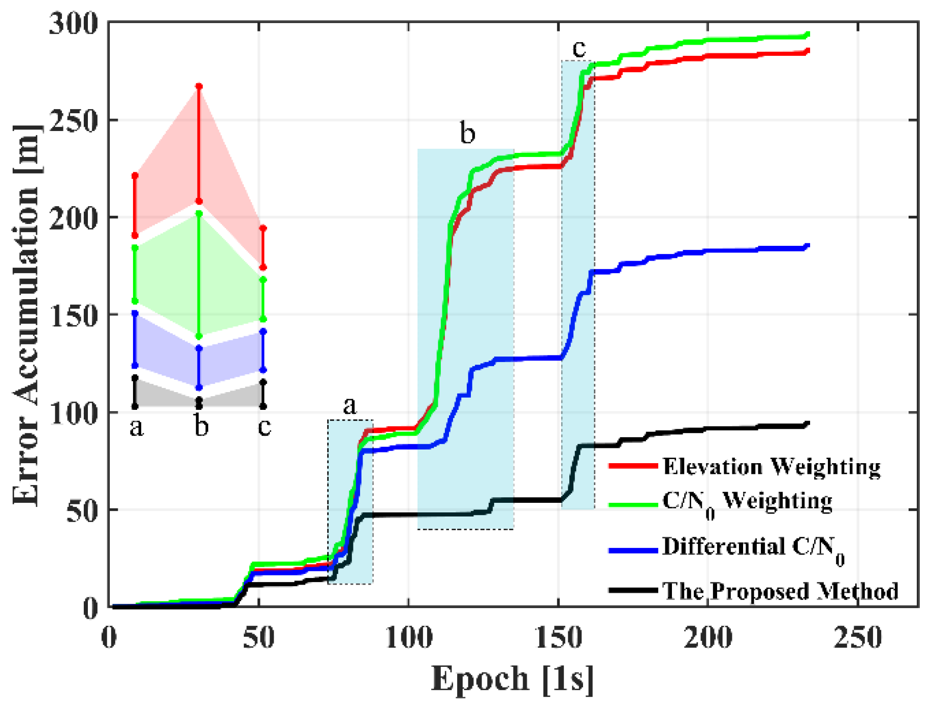
To further assess cumulative error growth over the full positioning process, we define an Error Accumulation (EA) index as
E A j i = 1 n = j G D j i
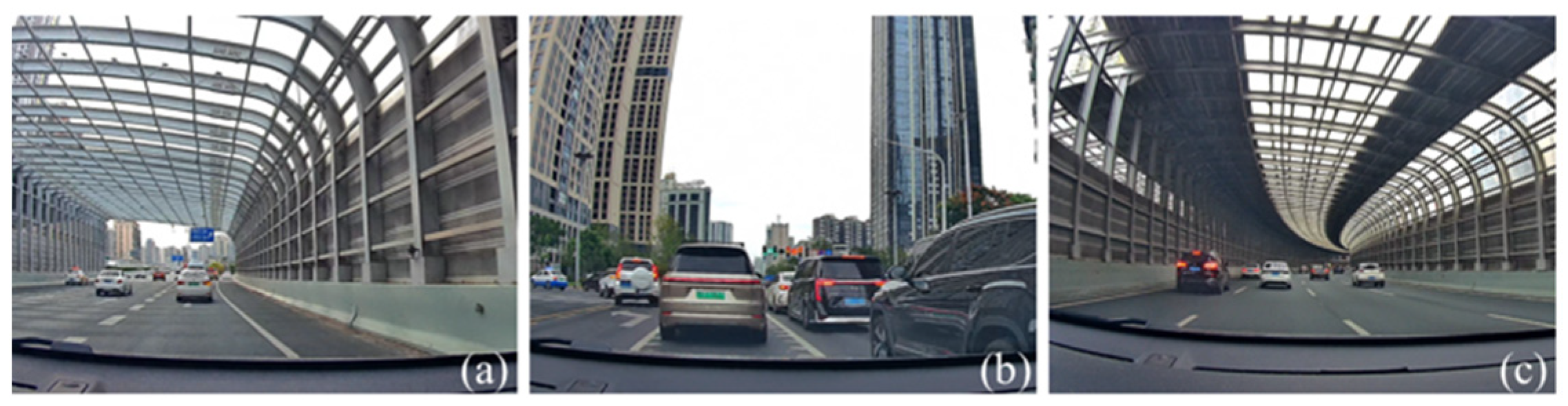
where i denotes the processing method and j denotes the epoch. Figure 18 shows the EA index for each method during the vehicle’s passage through the three severely obstructed events identified in Figure 19. The blue boxes in Figure 18 correspond to these critical segments: events (a) and (c) represent the outbound and return passes beneath a compartment-like structure located on an elevated roadway, with more severe blockage during event (c); event (b) corresponds to an urban crossroad surrounded by dense buildings.
As shown in Figure 18, the elevation-based and C/N0-based weighting models exhibit broadly similar error-accumulation behavior throughout the experiment. During the obstructed events, the EA index rises sharply and reaches approximately 280 m over the full test duration. Although the C/N0-based weighting model would generally be expected to mitigate errors to some degree under severe obstruction, the empirical parameters listed in Table 1 appear to be suboptimal for this dataset. In particular, during events (b) and (c), the EA index of the C/N0-based method is even higher than that of the elevation-based model, indicating degraded performance in more challenging environments. In addition, effective calibration of the C/N0-based model in kinematic positioning is difficult because satellite geometry, signal-propagation conditions, and environmental interference change continuously.
The differential C/N0 method performs better in kinematic positioning, with the Error Accumulation reduced to approximately 170 m because large outliers are effectively removed by differential thresholding. By contrast, the overall EA index of the proposed method is only about 94 m and remains the lowest across all three obstruction events, demonstrating superior ability to mitigate diffraction-induced errors.
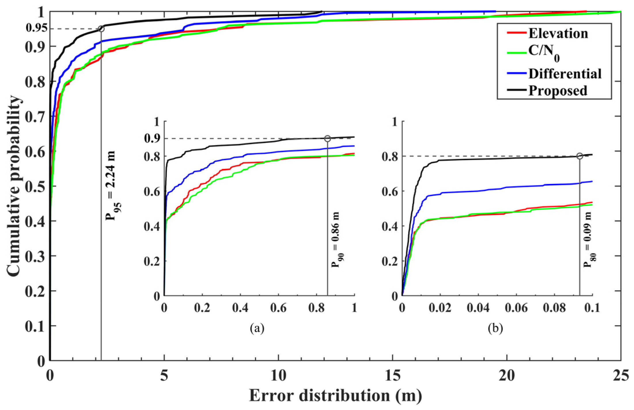
Figure 20 presents the cumulative distribution function (CDF) of the positioning errors. The elevation-based and C/N0-based weighting models show highly similar error-accumulation behavior throughout the experiment. In obstructed environments, the proposed method converges most rapidly toward 100% cumulative probability, with 95% of errors bounded within 2.3 m, 90% within 0.9 m, and 80% within 0.1 m. Notably, nearly 80% of the errors are smaller than 0.02 m, demonstrating a substantial improvement over the other three methods.

5. Discussion

The results from both the static and kinematic experiments show that the primary advantage of the proposed method is not merely a modest improvement in fixed-solution precision, but a substantial improvement in ambiguity-fixing availability, solution continuity, and overall robustness under severe obstruction. This behavior is physically consistent with the gradual development of diffraction error: observations affected by small or moderate diffraction still retain useful geometric information and are therefore better handled through adaptive down-weighting, whereas severely contaminated observations are more appropriately excluded.
A second important point concerns the distinction between the proposed method and the differential C/N0 strategy. The differential C/N0 method mainly functions as an outlier-rejection scheme once the inter-station C/N0 difference exceeds a threshold, whereas the proposed method introduces a severity-dependent transition from conventional weighting to combined down-weighting and, finally, to exclusion. This additional flexibility explains why the proposed method preserves higher data integrity in the static experiment and yields lower cumulative error growth in the vehicle-based experiment.
From an engineering perspective, the proposed approach is attractive because it can be implemented within the stochastic-modeling or pre-screening stage of existing RTK/PPP software without modifying the fundamental observation equations. At the same time, the open-sky templates and empirical thresholds are receiver- and environment-dependent. In practical deployment, recalibration is recommended whenever the antenna type, receiver firmware, satellite tracking characteristics, or urban morphology differs substantially from the calibration conditions adopted in this study.
It should also be emphasized that the operational indicator used in this study is a template-based C/N0 departure rather than a diffraction-only classifier. Similar C/N0 degradations may also be caused by severe shadowing, multipath, or receiver tracking degradation. In the two experiments analyzed here, however, the building-edge environments, the monotonic residual growth, and the simultaneous decrease in C/N0 are all consistent with the theoretical diffraction model, so the dominant errors are interpreted as diffraction-dominated NLOS effects. Nevertheless, for other cities, seasons, receiver firmware versions, or antenna gain patterns, the open-sky template and empirical thresholds should be recalibrated before operational deployment. Future work should combine the present C/N0-based screening strategy with richer geometric context or auxiliary sensing and validate the method using additional datasets collected under different seasonal and urban conditions.

6. Conclusions

Diffraction caused by signal blockage from tall buildings is a form of NLOS propagation that degrades GNSS positioning accuracy and compromises solution reliability. To address the challenge of precise positioning in urban environments with severe building obstruction, this study proposes a segmented weighting and elimination method for mitigating diffraction-induced errors. Open-sky data are first used to establish an elevation–C/N0 reference template. This template is then compared with real-time C/N0 measurements obtained in obstructed environments, and the resulting deviations are used to drive adaptive down-weighting or exclusion of carrier-phase observations. The proposed method was evaluated using both a static experiment under severe building shadowing and a vehicle-based kinematic experiment in urban scenarios.
In the static experiment, the proposed method outperforms the conventional elevation-based weighting model, the C/N0-based weighting model, and the differential C/N0 strategy. The ambiguity-fixing rate (AFR) exceeds 95%, compared with 50.8%, 52.6%, and 81.2% for the three comparison methods, respectively. The proposed method also delivers positioning accuracies of 4 mm in the horizontal component and 8 mm in the vertical component, demonstrating its effectiveness for high-precision applications under challenging urban conditions.
In the vehicle-based kinematic experiment, the proposed method achieves an AFR above 83%, substantially outperforming the elevation-based weighting model, the C/N0-based weighting model, and the differential C/N0 strategy, which achieve 38%, 44%, and 65.8%, respectively. Under severe obstruction, the cumulative positioning error of the proposed method remains consistently lower than that of the other methods. The method therefore provides a meaningful improvement over conventional down-weighting and exclusion strategies. Its principal practical benefit lies in improving ambiguity-fixing rate, continuity, and reliability in obstruction-dominated environments, whereas the improvement in already-fixed coordinate precision is more modest. This distinction is particularly relevant for engineering applications such as urban monitoring and vehicle-based positioning.

Author Contributions

X.M. contributed to the study conception and design. Software development and data processing were performed by R.X., B.X., J.G., X.Y. and N.H. carried out the data analysis. R.X. and X.M. drafted the manuscript. A.L. and K.G. supervised the study and commented on the manuscript. Material preparation and data collection were performed by X.D. and M.Y. All authors have read and agreed to the published version of the manuscript.

Funding

This study was supported by the Wuhan Natural Science Foundation Exploration Plan (Grant No: 2024040801020256), National Key Research and Development Program of China (Grant No: 2024YFC3810500), National Natural Science Foundation of China (Grant No. 42404021), Natural Science Foundation of Hubei Province (Grant No. 2024AFB232), and The Development and Application of Location-Based Service System in Canyon Area of Wudongde Hydropower Station (JG/19026B).

Data Availability Statement

The datasets generated during the current study are available from authors upon reasonable request (rjxi@whut.edu.cn).

Acknowledgments

The authors thank the RTKLIB open-source program package for providing the validation platform used in this study.

Conflicts of Interest

Authors Xin Meng, Bin Xiao, Jinsong Gao, Aijun Li, Xintao Yang, Kui Gao and Nianlong Han are employed by the company Wuhan Municipal Construction Group Co., Ltd. and Wuhan Municipal Environmental Engineering Construction Co., Ltd. Authors Xianyong Dong and Mengdi Yao are employed by the company China Three Gorges Construction Engineering Corporation. The remaining author declares that the research was conducted in the absence of any commercial or financial relationships that could be construed as a potential conflict of interest. The Wuhan Municipal Construction Group Co., Ltd., Wuhan Municipal Environmental Engineering Construction Co., Ltd. and China Three Gorges Construction Engineering Corporation had no role in the design of the study; in the collection, analyses, or interpretation of data; in the writing of the manuscript, or in the decision to publish the results.

Abbreviations

The following abbreviations are used in this manuscript:
3DMA3D Mapping Aided
AFRAmbiguity Fixing Rate
CDFCumulative Distribution Function
CNNConvolutional Neural Network
C/N0Carrier-Power-to-Noise-Density Ratio
DRLDeep Reinforcement Learning
EAError Accumulation
GDGeometric Distance
GNSSGlobal Navigation Satellite System
ICLInfimum Cut-off Line
LAMBDALeast-squares AMBiguity Decorrelation Adjustment
LiDARLight Detection and Ranging
LOSLine-of-Sight
LSTMLong Short-Term Memory
NLOSNon-Line-of-Sight
RFReconstruction Function
RMSERoot-Mean-Square Error
SVMSupport Vector Machine

References

  1. Zhong, P.; Ding, X.; Yuan, L.; Xu, Y.; Kwok, K.; Chen, Y. Sidereal filtering based on single differences for mitigating GPS multipath effects on short baselines. J. Geod. 2010, 84, 145–158. [Google Scholar] [CrossRef]
  2. Dong, D.; Wang, M.; Chen, W.; Zeng, Z.; Song, L.; Zhang, Q.; Cai, M.; Cheng, Y.; Lv, J. Mitigation of multipath effect in GNSS short baseline positioning by the multipath hemispherical map. J. Geod. 2015, 90, 255–262. [Google Scholar] [CrossRef]
  3. Hsu, L. Analysis and modeling GPS NLOS effect in highly urbanized area. GPS Solut. 2017, 22, 7. [Google Scholar] [CrossRef]
  4. Huang, G.; Du, S.; Wang, D. GNSS techniques for real-time monitoring of landslides: A review. Satell. Navig. 2023, 4, 5. [Google Scholar] [CrossRef]
  5. Chen, W.; Zhang, C.; Peng, Y.; Yao, Y.; Cai, M.; Dong, D. Enhancing GNSS positioning in urban canyon areas via a modified design matrix approach. IEEE Internet Things J. 2024, 11, 10252–10265. [Google Scholar] [CrossRef]
  6. Yuan, H.; Zhang, Z.; He, X.; Zeng, J.; Li, X. Resilient ambiguity resolution strategy in GNSS real-time kinematic positioning for urban environments. IEEE Internet Things J. 2024, 11, 30004–30013. [Google Scholar] [CrossRef]
  7. Satirapod, C.; Ogaja, C.; Wang, J.; Rizos, C. An approach to GPS analysis incorporating wavelet decomposition. Artif. Satell. 2001, 36, 27–35. [Google Scholar]
  8. Zheng, D.; Zhong, P.; Ding, X.; Chen, W. Filtering GPS time-series using a Vondrak filter and cross-validation. J. Geod. 2005, 79, 363–369. [Google Scholar] [CrossRef]
  9. Moschas, F.; Stiros, S. Measurement of the dynamic displacements and of the modal frequencies of a short-span pedestrian bridge using GPS and an accelerometer. Eng. Struct. 2011, 33, 10–17. [Google Scholar] [CrossRef]
  10. Shen, N.; Chen, L.; Wang, L.; Lu, X.; Tao, T.; Yan, J.; Chen, R. Site-specific real-time GPS multipath mitigation based on coordinate time series window matching. GPS Solut. 2020, 24, 82. [Google Scholar] [CrossRef]
  11. Zhang, Z.; Li, Y.; He, X.; Chen, W.; Li, B. A composite stochastic model considering the terrain topography for real-time GNSS monitoring in canyon environments. J. Geod. 2022, 96, 79. [Google Scholar] [CrossRef]
  12. Marais, J.; Berbineau, M.; Heddehaut, M. Land mobile GNSS availability and multipath evaluation tool. IEEE Trans. Veh. Technol. 2005, 54, 1697–1704. [Google Scholar] [CrossRef]
  13. Maier, D.; Kleiner, A. Improved GPS sensor model for mobile robots in urban terrain. In Proceedings of the IEEE International Conference on Robotics and Automation, Anchorage, AK, USA, 3–7 May 2010; pp. 4385–4390. [Google Scholar]
  14. Zimmermann, F.; Eling, C.; Kuhlmann, H. Empirical assessment of obstruction adaptive elevation masks to mitigate site-dependent effects. GPS Solut. 2017, 21, 1695–1706. [Google Scholar] [CrossRef]
  15. Hsu, L.; Gu, Y.; Kamijo, S. 3D building model-based pedestrian positioning method using GPS/GLONASS/QZSS and its reliability calculation. GPS Solut. 2016, 20, 413–428. [Google Scholar] [CrossRef]
  16. Xin, S.; Geng, J.; Zhang, G.; Ng, H.; Guo, J.; Hsu, L. 3D-mapping-aided PPP-RTK aiming at deep urban canyons. J. Geod. 2022, 96, 78. [Google Scholar] [CrossRef]
  17. Suzuki, T.; Matsuo, K.; Amano, Y. Rotating GNSS antennas: Simultaneous LOS and NLOS multipath mitigation. GPS Solut. 2020, 24, 86. [Google Scholar] [CrossRef]
  18. Xi, R.; Xu, D.; Jiang, W.; He, Q.; Zhou, X.; Chen, Q.; Fan, X. Elimination of GNSS carrier phase diffraction error using an obstruction adaptive elevation masks determination method in a harsh observing environment. GPS Solut. 2023, 27, 139. [Google Scholar] [CrossRef]
  19. Han, J.; Huang, G.; Zhang, Q.; Tu, R.; Du, Y.; Wang, X. A new Azimuth-dependent elevation weight (ADEW) model for real-time deformation monitoring in complex environment by multi-GNSS. Sensors 2018, 18, 2473. [Google Scholar] [CrossRef]
  20. Ren, H.; Li, G.; Geng, J.; Wang, F.; Li, P. Multipath hemispherical map model with geographic cut-off elevation constraints for real-time GNSS monitoring in complex environments. GPS Solut. 2023, 27, 188. [Google Scholar] [CrossRef]
  21. Xi, R.; Han, L.; Chen, Q.; Jiang, W.; Meng, X.; An, X.; Xuan, W. Numerical modeling and analysis of GNSS carrier-phase diffraction error in occlusion environments. J. Geod. 2025, 99, 32. [Google Scholar] [CrossRef]
  22. Liu, Q.; Gao, C.; Shang, R.; Peng, Z.; Zhang, R.; Gan, L.; Gao, W. NLOS signal detection and correction for smartphone using convolutional neural network and variational mode decomposition in urban environment. GPS Solut. 2023, 27, 31. [Google Scholar] [CrossRef]
  23. Li, F.; Zhai, C.; Xie, T.; Dai, Z.; Zhu, X. GNSS positioning enhancement based on NLOS signal detection using spatiotemporal learning in urban canyons. GPS Solut. 2024, 28, 209. [Google Scholar] [CrossRef]
  24. Sun, R.; Wang, G.; Zhang, W.; Hsu, L.T.; Ochienge, W.Y. A gradient boosting decision tree based GPS signal reception classification algorithm. Appl. Soft Comput. 2019, 86, 105942. [Google Scholar] [CrossRef]
  25. Hsu, L. GNSS multipath detection using a machine learning approach. In Proceedings of the IEEE 20th International Conference on Intelligent Transportation Systems 2017 (ITSC), Yokohama, Japan, 16–19 October 2017; p. 17631909. [Google Scholar]
  26. Lyu, Z.; Gao, Y. An SVM based weight scheme for improving kinematic GNSS positioning accuracy with low-cost GNSS receiver in urban environments. Sensors 2020, 20, 7265. [Google Scholar] [CrossRef] [PubMed]
  27. Tang, J.; Li, Z.; Yu, Q.; Zhao, H.; Zeng, K.; Zhong, S.; Wang, Q.; Xie, K.; Kuzin, V.; Xie, S. Deep reinforcement learning with robust augmented reward sequence prediction for improving GNSS positioning. GPS Solut. 2025, 29, 65. [Google Scholar] [CrossRef]
  28. Li, Z.; Cao, M.; Zeng, K.; Wang, Q.; Xie, K.; Xie, S. A graph contrastive learning-based semi-supervised GNSS NLOS signal recognition method. GPS Solut. 2026, 30, 42. [Google Scholar] [CrossRef]
  29. Melbourne, W.G. The case for ranging in GPS based geodetic systems. In Proceedings of the 1st International Symposium on Precise Positioning with the Global Positioning System, Rockville, MD, USA, 15–19 April 1985; pp. 373–386. [Google Scholar]
  30. Xiong, Y.; Ding, X. Mitigation of GPS signal diffraction effect for deformation applications based on environment modelling. Acta Geod. Cartogr. Sin. 2005, 34, 283–287. [Google Scholar]
  31. Dai, W.; Ding, X.; Zhu, J. Single reflected or diffracted signal error elimination method in GPS dynamic deformation monitoring. J. Geotech. Investig. Surv. 2006, 34, 45–49. [Google Scholar]
  32. Brunner, F.K.; Hartinger, H.; Troyer, L. GPS signal diffraction modelling: The stochastic SIGMA-Δ model. J. Geod. 1999, 73, 259–267. [Google Scholar] [CrossRef]
  33. Lau, L.; Cross, P. Development and testing of a new ray-tracing approach to GNSS carrier-phase multipath modelling. J. Geod. 2007, 81, 713–732. [Google Scholar] [CrossRef]
  34. Jiang, Z.; Groves, P.D. NLOS GPS signal detection using a dual-polarisation antenna. GPS Solut. 2014, 18, 15–26. [Google Scholar] [CrossRef]
  35. Xi, R.; Chen, Q.; Meng, X.; Jiang, W.; An, X.; He, Q. A multi-GNSS differential phase kinematic post-processing method. Remote Sens. 2020, 12, 2727. [Google Scholar] [CrossRef]
  36. Teunissen, P.J.G. The least-squares ambiguity decorrelation adjustment: A method for fast GPS integer ambiguity estimation. J. Geod. 1995, 70, 65–82. [Google Scholar] [CrossRef]
  37. Kuusniemi, H.; Wieser, A.; Lachapelle, G.; Takala, J. User-level reliability monitoring in urban personal satellite-navigation. IEEE Trans. Aerosp. Electron. Syst. 2008, 43, 1305–1318. [Google Scholar] [CrossRef]
  38. Han, L.; Xi, R.; Chen, Q.; Xiao, Y.; Wang, K.; Xu, D.; Jiang, W. Analysis and elimination of GNSS carrier phase diffraction error in high occlusion environments. Measurement 2025, 253, 117809. [Google Scholar] [CrossRef]
Figure 1. Diagram of GNSS diffraction effect.
Geomatics 06 00058 g001
Figure 2. The geometric structure of the horizontal (a,b) and vertical (c,d) diffraction effect when the satellite signal transmits to a vertical and a horizontal edge of a building.
Geomatics 06 00058 g002
Figure 3. Diffraction errors increase with respect to the diffraction angle. (a) is the horizontal diffraction, and (b) is the vertical diffraction.
Geomatics 06 00058 g003
Figure 4. Carrier phase residuals (in black lines), C/N0 (in blue lines), elevation time series (in green lines) and the model of diffraction observations for GPS G32 (horizontal diffraction) and BDS C28 (vertical diffraction) in red lines. The shadow area shows the diffraction time series.
Geomatics 06 00058 g004
Figure 5. “Elevation–C/N0” measurement fitting model for the GPS (A), Galileo (B), BDS-IGSO (C) and BDS-MEO (D) satellite data collected in an open environment.
Geomatics 06 00058 g005
Figure 6. C/N0-based segmented weighting and elimination diagram. The black dashed line indicates the fitting curve of the “elevation–C/N0” correlation model. The black solid line denotes the reconstructed model, also referred to as the Reconstruction Function (RF). The red line denotes the lower boundary of the model, also referred to as the Infimum Cut-off Line (ICL). The blue, yellow, and green areas indicate the conventional elevation-weighting, down-weighting, and elimination regions, respectively.
Geomatics 06 00058 g006
Figure 7. Experimental location and photograph of GNSS observing conditions of stations.
Geomatics 06 00058 g007
Figure 8. The probability density distribution and the frequency distribution histogram of the C/N0 time series of GPS (A), Galileo (B), BDS-IGSO (C) and BDS-MEO (D) satellites collected in an open environment. The depth of the color represents the value of the distribution of probability. The frequency distribution histograms of the C/N0 are shown on the left side of each plot, and the ordinate represents the percentage of the C/N0 within an interval of 1 dB-Hz as the total number.
Geomatics 06 00058 g008
Figure 9. Rover station setup, data collection, and photographs of the observing environment.
Geomatics 06 00058 g009
Figure 10. C/N0 sky-plot of the rover station.
Geomatics 06 00058 g010
Figure 11. Positioning results obtained with the elevation-based and C/N0-based weighting methods.
Geomatics 06 00058 g011
Figure 12. C/N0 measurements with respect to elevation angle for GPS-G04, GAL-E30, BDS-C39, and BDS-C36. The black solid lines indicate the RF line, and the dark red dashed lines denote the ICL. The blue dots denote the conventional elevation-weighting zone, the yellow dots denote the combined elevation- and C/N0-based down-weighting zone, and the green dots denote observations excluded during data processing. The symbols in the right panel indicate the trajectories of GPS-G04 (G), GAL-E30 (E), BDS-C39 (I), and BDS-C36 (M).
Geomatics 06 00058 g012
Figure 13. Data processing results of the proposed method and the differential C/N0 strategy.
Geomatics 06 00058 g013
Figure 14. Histogram of the a posteriori residuals for GPS, Galileo, and BDS. In the figure, ‘K’ denotes kurtosis and ‘S’ denotes skewness.
Geomatics 06 00058 g014
Figure 15. Driving route of the vehicle-based experiment.
Geomatics 06 00058 g015
Figure 16. Obstructed environments encountered in the vehicle-based experiment.
Geomatics 06 00058 g016
Figure 17. Geometric-distance (GD) time series (blue dots) obtained with the elevation-based weighting method (A), the C/N0-based weighting method (B), the differential C/N0 method (C), and the proposed method (D). The shaded region denotes the interval during which the vehicle passed through a dense urban intersection, and the red dots are the usable solutions during this interval.
Geomatics 06 00058 g017
Figure 18. EA index for the four methods. The red, green, blue, and black lines indicate the elevation-based weighting method, the C/N0-based weighting method, the differential C/N0 method, and the proposed method, respectively. The three blue boxes indicate the obstruction events shown in Figure 19.
Geomatics 06 00058 g018
Figure 19. Photographs of the three obstruction events. Events (a,c) represent the outbound and return passes beneath a compartment-like structure located on an elevated roadway, event (b) corresponds to an urban crossroad surrounded by dense buildings.
Geomatics 06 00058 g019
Figure 20. Cumulative distribution function (CDF) of the four methods. The curve colors are the same as those used in Figure 18.
Geomatics 06 00058 g020
Table 1. Data processing strategies.
Models or ParametersStrategies
ObservationsGPS: L1/L2, BDS: B1/B3, Galileo: E1/E5a
Cut-off elevation10°
EphemerisBroadcast ephemeris
EstimatorKalman filter
Ambiguity resolutionLeast-squares AMBiguity Decorrelation Adjustment (LAMBDA) method [36]
Ratio threshold2.2 (empirical value selected to balance fix availability and reliability in severe urban obstruction)
Diffraction error processing schemeA: Elevation-based weighting model, w = 1 / σ e l e 2 , where σ e l e 2 = a 2 + b 2 / sin 2 θ and a = b = 3   mm ;
B: C/N0-based weighting model, w = 1 / σ s n r 2 , where σ s n r 2 = c 2 + d · 10 C / N 0 10 , and c = 3   mm and d = 150 2   mm 2 Hz [37];
C: Differential C/N0 method [38];
D: Proposed method.
SoftwareRTKLIB-based in-house post-processing platform with a custom stochastic weighting/elimination module
Template calibrationOpen-sky short baseline (107.00 m); templates built for GPS, Galileo, BDS-IGSO, and BDS-MEO classes
Template screening thresholdτ = 1.7 (selected from the open-sky calibration dataset to reject strongly fluctuating arcs)
Differential C/N0 threshold5 dB-Hz (empirical short-baseline rejection threshold)
Low C/N0 exclusion threshold35 dB-Hz (empirical lower carrier-tracking bound for the K803 + geodetic antenna setup)
Table 2. Statistics of the data processing results.
MethodsAFRAverage RatioData IntegrityNum.PDOPRMSE (mm)
ENU
Elevation weighting50.8%3.3081.93%28.031.17---
C/N0-based weighting52.6%3.7981.93%28.031.17---
Differential C/N081.2%9.0781.93%23.181.283.13.98.7
The proposed method95.5%11.8599.01%24.261.212.93.88.6
Table 3. AFR and positioning-accuracy statistics for the four methods.
StrategiesElevation WeightingC/N0-Based WeightingDifferential C/N0The Proposed Method
AFR38.2%44.3%65.8%83.6%
GD-RMSE2.196 m1.788 m1.470 m0.751 m
Disclaimer/Publisher’s Note: The statements, opinions and data contained in all publications are solely those of the individual author(s) and contributor(s) and not of MDPI and/or the editor(s). MDPI and/or the editor(s) disclaim responsibility for any injury to people or property resulting from any ideas, methods, instructions or products referred to in the content.