Workflow of Visualisation of Mole-Rat Burrows Using 3D Datasets Derived from GPR, UAV Surveys, and Interpretative Processing

Highlights

What are the main findings?

• Three-dimensional model of animal burrows.
• Joint visualisation of UAV and GPR datasets in one platform.
• A processing workflow of complex 3D datasets into an easily workable text file (*.CSV).

What are the implications of the main findings?

• Easily, visually interpretable 3D datasets as one object.
• Universally compatible *.CSV data type.
• Storage of complex information in a simplified format.
• An unlimited number of covariates and auxiliary variables can be assigned to the primary data.

Abstract

We present a concise methodology to model and visualise mole-rat burrows by integrating 3D ground-penetrating radar (GPR) volumes, high-resolution 3D surface texture, and interpretative 3D visualisation with open-code software, such as Blender and Houdini. The workflow shows the processing and conversion steps for converting surface and subsurface raw datasets into point clouds, then the amalgamation of those 3D objects into a voxelised volume. The voxelisation script creates a text file, a *.CSV file, that masks the voxels with the values of 0 and 1 depending on whether they are inside or outside a burrow. This parametrisation resulted in a total of 7,730,587 voxels generated, of which 48,952 have a value of 1 within them. This indicates the presence of one burrow system, in which there were about 60–80 burrow segments that were initially identified by GPR but remained rather interpretative than a verified geometry. The entire process enables handling and combining different, complex, 3D datasets into a simple text file and thus enables merging with covariates for further spatial modelling of burrow systems from incomplete, indirect, noisy measurements.

1. Introduction

Underground animal burrows profoundly influence soil structure, hydrology, nutrient cycling, surface morphology, and ecosystem functions and services provided by the soil. This can occur via different mechanisms, including increased aeration and watering of the soil ecosystem, providing habitat and resting places for other vertebrates or invertebrates, and mixing different soil horizons [1,2,3,4,5,6,7]. One of the most well-known, endangered burrowing mammals in Eurasian steppe-like or mountain grasslands is the lesser blind mole-rat superspecies (Nannospalax leucodon), containing several cryptic species [8]. Their subterranean burrow systems alter soil porosity and aggregate stability, redistribute nutrients, and affect vegetation patterns across landscapes. As a result of their crucial role in the ecosystem and their protected status in several countries, it is important to be able to give accurate estimates of the area occupied by a colony and of the abundance of individuals within it [9,10,11,12]. However, due to their fossorial lifestyle, observation of specimens is infeasible, and hence estimation of their abundance should look at other means of relevant quantitative indicators of their presence in an area. Mounds are distinctive and obvious indicators of their presence in an area and are directly related to individual abundance. Animals leave mounds behind while they are digging their burrow systems during feeding or moving underground. Mounds are used as proxies of their presence because they enable quantitative, relative estimation of individual abundance in colonies. Nevertheless, accurate estimation of the number of mounds belonging to one burrow system or individual is a challenging task. If that mound number could be estimated more accurately, then this could be converted into a more accurate individual abundance of a colony [3,13,14,15].

Traditional approaches to studying above- and below-ground burrow systems or the animals that create them include methods such as manually recording the number and location of burrows and mounds, excavating burrow systems, and trapping animals. However, these methods are often infeasible, particularly over large areas. They can also be labour-intensive, destructive, and raise ethical concerns. In the case of endangered species, such approaches may even be prohibited. Consequently, non-destructive, proximal surface or subsurface sensing methods, such as conservation Unpiloted Aerial Vehicles (UAV), Ground Penetrating Radar (GPR), and advanced 3D image processing and modelling techniques, become increasingly popular, valuable tools for detecting, counting, and mapping both surface burrow mounds or openings and subsurface animal burrows [16]. Whilst identification, detection, and counting of surface mounds and identification of subsurface burrows have already been performed successfully, they have not been fully developed or combined with other proximal sensing methods for use in on-the-ground conservation practice [13]. Discrete techniques are applied to answer different questions related to animals’ distribution, burrowing, abundance, or habitat engineering. These techniques often require different tools and approaches, necessitating often expensive processing software for handling data collected during surveys.

Our aim is to combine non-destructive, proximal sensing methods, 3D datasets, and interpretive software for the visualisation of joint datasets, representing burrow systems both above and below ground. With this methodology, we could give an impetus to developing a semi-automated methodology that could non-destructively map the burrow system in 3D and real time, and that information could eventually be used in more accurate estimates of individual density, soil mixing, and habitat engineering of mole-rats or species alike.

1.1. UAV Imaging, Digital Terrain Model (DTM)

UAVs equipped with various sensors, such as RGB cameras, multispectral or hyperspectral imaging spectrometers, and laser scanners, have proven useful for environmental and ecological research projects, particularly for local or regional studies or when rapid data acquisition is required [17]. Combining a wide range of sensors with a low flight altitude (below 100 m) results in centimetre-level spatial resolution in the produced data, irrespective of whether this is imagery or topography. This makes the UAVs useful for monitoring small mammals, such as rodents, and their habitats with subsurface objects, such as burrows, holes, or mounds. From a sensor’s perspective, they have all proven useful for detecting such features, while RGB cameras are probably the most widely used due to their simplicity and ease of processing [13,17,18,19]. The main purpose of imaging sensors is to record the differing spectral characteristics of soil ‘patches’, mounds, and the surrounding vegetation (e.g., grass and bushes), or dry topsoil. However, it is also possible to generate the topography of the habitats under investigation and locate the burrows and mounds geometrically in the produced digital terrain or surface model using morphological layers and filters [20].

1.2. GPR Surveying, 3D Subsurface Model

GPR can detect small discontinuities in dielectric permittivity or constants of the soil medium, including different materials, layers, or voids in the soil [21,22,23]. If conditions are adequate for a GPR survey, it can provide a detailed cross-sectional image of subsurface burrows [24]. However, without additional information about the area surveyed by GPR and when it is used exclusively, GPR data can be challenging to interpret, especially when signals recorded by the receiver antenna are weak, discontinuous on images, or masked by other effects that may produce similar reflections on the radargrams.

Three-dimensional (3D) GPR surveying and data processing, compared to 2D surveying, improve the ability to reconstruct subsurface geometries by integrating dense radar line scans into volumetric datasets. Moreover, 3D visualisation allows us to trace continuous anomalies like burrows [25,26]. If we could map a large part of the burrow system, then we would be able to quantitatively estimate its various characteristics, such as volume, longitudinal trajectory, and curvature. However, even with advanced processing workflows and experience, GPR-derived models alone remain difficult to interpret and visualise.

1.3. Processing 3D Point Clouds and Polygons

In 3D visualisation of objects, where internal structure and geometry are an important part of the object’s visualisation, SideFX Houdini 21.0.512 Apprentice and Blender 5.0 serve as complementary platforms for modelling, simulating, and rendering complex spatial objects. SideFx Houdini is a widely utilised visual effect (VFX) software within the 3D industry [27,28,29]. The built-in modules facilitate the straightforward modification of the existing models’ or objects’ coordinates and shapes through the utilisation of mathematical formulas. Houdini applies a node-based operational system in which every modification is represented as a discrete node connected in a network. Each node performs a specific operation, such as generating a geometry, importing data, or computing a volumetric shape, and the connections between nodes define the sequence of transformations applied to the entire 3D object. An advantage of this approach is that the sequence of transformations is stored as a graph, in which the user can modify any parameter at any node, and the changes are then automatically propagated through the network. This makes Houdini a powerful tool for visualisation tasks where reproducibility, parameter control, and iterative refinement are essential [30,31]. For example, if the burrow’s width within the object is modified, then this new value of the burrow’s diameter updates the entire burrow model without the need for rebuilding the system. This same logic and approach apply to mechanical assemblies, biological structures, or any 3D object where internal geometry should be visualised consistently.

Blender is also an increasingly prevalent software in the 3D industry, particularly in light of recent developments [32]. It is characterised by its accessibility and relative ease of usage by non-specialists. The integration of Python (version 3.12) codes facilitates the execution of even the most intricate operations and calculations in a swift manner. Blender 5.0 supports efficient creation of cross-section views, transparent materials, and animated cross-sections that visualise interior–exterior relationships [33,34,35].

Together, these tools allow the visualisation of 3D bodies by combining sequential procedures and merging, subtracting or intersecting 3D objects to produce images suitable for further imaging or spatial modelling [36].

In this paper, we want to illustrate the steps taken for developing a 3D burrow model of a mole-rat burrow system surveyed in Shistavec, northeastern Albania, in an alpine grassland [37]. This paper aims to explain the steps and demonstrate the advantages of combining the above-mentioned techniques to develop the best available 3D model or map of a mole-rat burrow system. The steps taken involve generating the following datasets and processing: 1. Applying aerial photographs with RTK GPS to produce a DTM and orthophoto of an area of interest. The DTM includes information on the surface features, shapes, geometry, and elevation gradient of the mounds. 2. Surveying the underground burrow systems using GPR. For this task specifically, 3D surveying is used to provide the best volumetric image of the burrows. 3. Using freely available open-source software packages to model the burrows derived from the GPR. The first processing phase of burrow modelling was performed in SideFx Houdini 21.0.512 Apprentice, while the second phase was performed in Blender 5.0. These 3D-point cloud processing software packages can integrate the DTM point cloud and the GPR polygon formats into one object, supplementing one another. 4. Finally, using the surface and subsurface bodies and interim results of processing steps to provide a merged 3D object built from voxels, including the burrow system and coded binary representation of mole-rat burrows (value “1”) and anything else (value “0”). That binary-coded 3D object is then converted into a *.CSV file containing the spatial information of the burrow system (spatial relationships and location), which enables further quantitative analysis and processing, such as spatial modelling and predicting the likelihood of presence of the burrow system in unsurveyed segments.

2. Materials and Methods

2.1. Study Site and Data Acquisition Tools

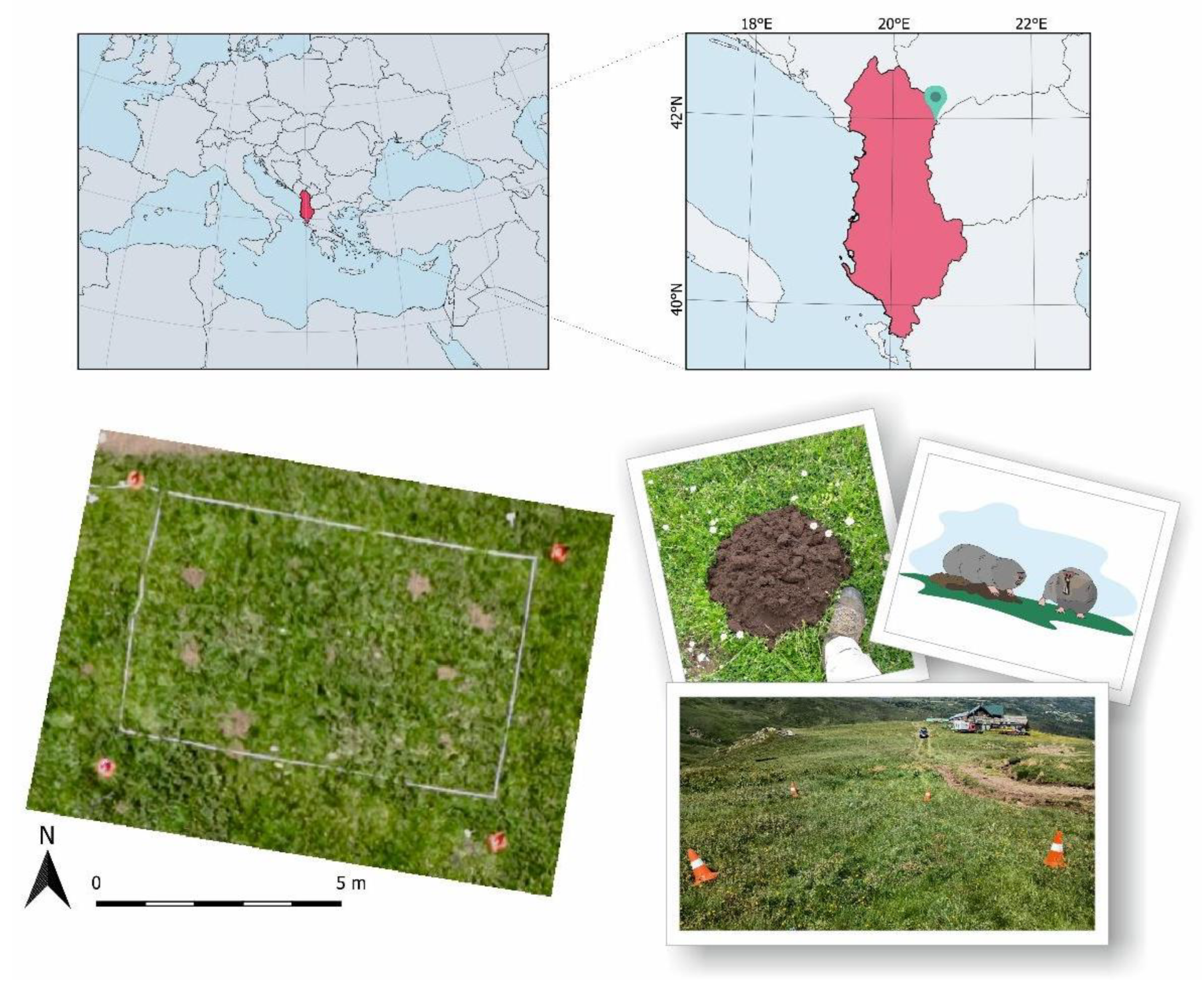
We conducted our research near Shishtavec and Bafa villages (Kukës region, Albania), in the proximity of the Skiatori Ski Resort, in a mountain grassland at an elevation of approximately 1820 m a.s.l. (Figure 1). The survey location was at 41.9457° N, 20.6110° E (WGS84). The habitat of the mole-rat colony represented a typical mountainous grassland, consisting of short vegetation (<0.1 m), enabling the detection and identification of animal mounds [13]. The size and quasi-circular shape of the mounds (>0.2 m = r) on the 3D grid enabled their easy identification by the naked eye.

Our field work involved a Mavic 3 Enterprise (DJI, Shenzhen, China) unmanned aerial vehicle (UAV) to survey the area of approximately 10 ha (400 m × 250 m). The other field equipment was a ground penetrating radar (GPR) system including a UtilityScan Dual Frequency (300/800 MHz) antenna (GSSI, Nashua, NH, USA), Panasonic G2 Toughpad (Newark, NJ, USA) embedded with the needed software to carry out the survey, a 4-wheel cart, a Reach RS2+ GPS (Emlid, Budapest, Hungary) and a compatible tripod for mounting to the GPR, and necessary additional cables and batteries. To achieve better accuracy between the GPR and UAV data, a second GPS receiver (a Galaxy G1 [SOUTH GNSS, Guangzhou, China]) was placed on a nearby fixed tripod to act as a temporary local GPS base station. The GPR and UAV systems both had independent positions relative to this second GPS unit via post-processing.

We corrected the discrepancy between the GPR and UAV data that arose during the transformation into the raw local coordinate system by manually aligning the data in Blender. Manual alignment was aided by the white stripe on the sample area (Figure 1). By manually adjusting the datasets within Blender, we were able to align these shared morphological elements with centimetre precision. The human eye is effective at recognising fine-scale geometric correspondences that algorithms may overlook or mismatch when positional metadata contains small systematic errors or blurred images. By zooming in (to pixel scale) and adjusting the datasets interactively, the operator was able to exploit these shared morphological cues to achieve a precise, context-based fit that is difficult to reproduce with automated algorithmic methods. This makes human-guided co-registration a robust and efficient solution when fine-scale structural matching is required; however, an RTK-based location georeferencing within both datasets could enable a less laborious and accurate automated way to merge, analyse, and interpret otherwise separate, georeferenced images of animal burrows. To quantify the accuracy of the manual alignment, we used the root mean square error (RMSE), a standard metric that expresses the average magnitude of the residual deviations.

We determined the errors based on the discrepancy between the coordinates of the corner points marked with white bands on the digital terrain model (DTM) and the coordinates of the corner points of the area delineated by the GPR data. First, we performed the RMSE calculation on the DTM and GPR objects already in the local coordinate system, and then on the manually corrected GPR data.

We calculated the RMSE value in Houdini, as this software is better suited for such operations than Blender. In this method, the script used in Houdini first determines the distance between the closest corner points of the DTM and GPR along the X and Y axes, then performs an RMSE calculation:

$$dx,dy=\sqrt{Pa.x,y^2-Pb.x,y^2}$$

where dx and dy are the distances between the points, Pa.x,y represents the x and y coordinates of the given point of the first imported object, while Pb.x,y represents the coordinates of the given point of the second imported object.

$$RM{SE}_{x,y}=\sqrt{{\displaystyle \frac{1}{n}}\sum _{i=0}^{n-1}{d}_{x,y}^2}$$

where RMSE_x,y is the error of the x and x coordinates, n is the number of points (in this case, 4), and d_x,y is the distance on the x and y coordinates.

Before manual transformation, the RMSE value measured along the X-axis was 6.85 m, while the RMSE value measured along the Y-axis was 2.91 m. This significant discrepancy was likely due to the different coordinate systems of the GPR and DTM data. Following the transformation process, the RMSE value of the 4 examined coordinates decreased to 0.27 m along the X-axis and 0.07 m along the Y-axis. The RMSE values for the GPR data in the local coordinate system and the manually corrected GPR coordinates were 6.68 m along the X-axis and 2.88 m along the Y-axis. This manual adjustment improved the reliability and interpretability of the subsurface burrow segments by ensuring better alignment between the surface DEM and the segments’ passages.

2.2. UAV Survey and Processing

We conducted the aerial survey at the site using a Mavic 3E (DJI, Shenzhen, China) with a visible range (RGB) camera onboard and an additional Real-Time Kinematic (RTK) antenna (DJI, Shenzhen, China). Its main sensor took RGB images 5280 px wide by 3956 px high with other parameters set to automatic (ISO speed and shutter speed) or as constant (focal length of 12.29 mm, aperture of f/2.8) value. The aerial survey was performed in a fully automatic flight mode above the habitat area with an image overlap of 80% and a sidelap of 50% to ensure photogrammetric processing. Flight altitude of 75 m was found adequate, together with set image resolution and focal length, to produce digital representations of the area with an approximately 0.025 m/pixel spatial resolution, sufficient for recording mounds in detail on several pixels. Using the local GPS base station together with the drone-board RTK antenna and GPS unit, it was possible to retain the UAV’s positioning information with centimetre accuracy.

The raw images were processed later in a photogrammetric workflow, performed in Agisoft Metashape Professional (version 1.8), to generate a georeferenced digital surface model and orthophoto mosaic of the habitat. Final datasets were exported into GeoTIFF format with UTM/WGS84 zone 34 coordinate system at 0.025 m/pixel spatial resolution. At this scale, one average mound with a diameter of approximately 0.3–0.4 m covered 80–100 pixels. Later, the specific area surveyed by GPR was clipped from both datasets to support the modelling steps.

2.3. GPR Survey

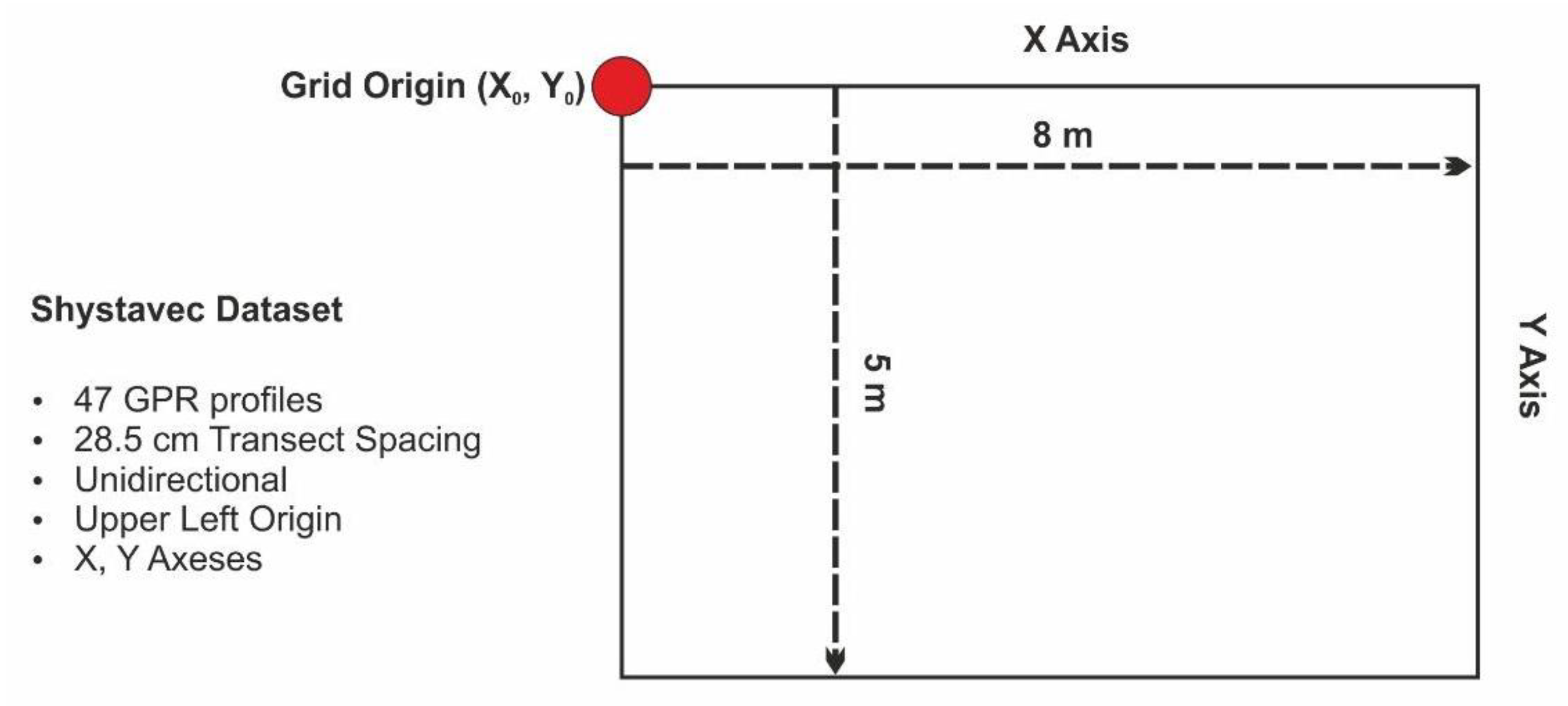
The GPR dataset was collected over a rectangular 8 m × 5 m grid, using parallel line transects spaced at 0.285 m and a scan density of 150 scans per metre; therefore, trace spacing was 0.00667 m, based on the relationship between scan rate, scan density, and survey speed. (Trace spacing is equal to the inverse of Scan density.)

$${\displaystyle \frac{Scan rate (\mathrm{s}\mathrm{c}\mathrm{a}\mathrm{n}\mathrm{s}/\mathrm{s})}{Survey speed (\mathrm{m}/\mathrm{s})}}=Scan density (\mathrm{s}\mathrm{c}\mathrm{a}\mathrm{n}\mathrm{s}/\mathrm{m}\mathrm{e}\mathrm{t}\mathrm{e}\mathrm{r})$$

The net time spent on the GPR data acquisition was approximately 3–4 h, which did not include travel time to the site and the set-up of the local GPS base unit for coordinate correction. Surveys indicated an approximate penetration depth of about 1 m, which was enough to identify most subsurface burrows in the surveyed area, though without being able to verify our findings in the field, they represented interpreted anomalies rather than a verified burrow geometry. Mole-rat burrows had a diameter of 0.07–0.1 m. The 3D-survey grid was on a gently sloping mountain grassland characterised by short grass (<0.1 m). Piles of mounds were flattened after the UAV survey to minimise surface obstruction and facilitate ground-coupled GPR acquisition. For horizontal RTK-GPS positioning of GPR scans, the GPS was fixed to the cart above the antenna. This provided accuracy to within one centimetre horizontally and vertically. Direction of line scans were up the hill (“x”) and laterally (“y”). Direction X was the 8 m side of the rectangular (Figure 2).

2.3.1. Soil and Environmental Conditions

The survey took place in summer; consequently, soil moisture was moderate or light during the study. The soil in this area was shallow, well-drained loamy soils with scattered gravel and small stones, typical of high-elevation grasslands in this region. Since the estimated penetration depth was about 1 m, the dual-frequency antenna was appropriate, and the conditions indicated that we were able to cover a significant part of the depth range of mole-rat burrows because burrows usually run within the upper 1 m of the soil profile [38].

2.3.2. GPR Data Processing

Processing of GPR data in RADAN 7 software (GSSI) started with the Global Settings set, first, for Utility Scan mode. Then, to speed up processing data and enable larger flexibility in optimising data images for later interpretation, we changed the set-up to Standard view mode. Data processing followed the general instructions of RADAN 7 manuals for Utility Scan and 3D data processing aimed at shallow subsurface surveying and imaging. The aim of data processing was to enhance signal quality, minimise background noise, and optimise the visibility of subsurface burrows before the 3D visualisation and interpretation. The final subsurface volume was exported in *.DXF format for further external processing in other applications.

A GSSI dual-frequency DF300/800 GPR system was used; however, the 800 MHz centre frequency antenna, channel 2, and corresponding data have provided the best resolution for the target, namely, the animal burrows. As a result of this and distinct processing and filtering characteristics for each centre frequency, such as different gain characteristics, the IIR filter was applied to the D50800 antenna. This approach to processing provided better visibility and interpretation of the data. The survey covered an 8 × 5 m area using a 3D grid layout with 28.5 cm line (transect) spacing. Data were acquired in unidirectional mode with a horizontal sampling rate of 150 scans * s⁻¹, corresponding to 100 scans * m⁻¹ (Figure 2).

Vertical sampling parameters included 512 samples per scan at 32-bit resolution. A time window (range) of 15 ns was used, and a dielectric constant (${\epsilon }_r$) of 11 was assumed for soil characteristics and depth conversion. The dielectric constant was used to calculate the propagation velocity in the soil and the depth of burrows. From those parameters, wave velocity (v) was approximately 0.090 m * s⁻¹ (${\displaystyle \frac{c}{\surd {\epsilon }_r}}=v;c is approximately 0.3 \mathrm{m}\ast {\left(\mathrm{n}\mathrm{s}\right)}^{-1}$). Consequently, the maximal depth was approximately 0.68 m (${ Depth}_{max}={\displaystyle \frac{0.090\ast 15}{2}}$). To sum up, two-way travel time was converted to depth (m) using wave velocity derived from the assumed dielectric constant. The 15 ns time window and 512 vertical samples, therefore, defined the maximum reachable depth and the vertical sampling interval.

Additional processing details included the following steps:

Time-Zero Correction

Time-zero correction or alignment was performed to synchronise the first arrival of the direct ground wave across profiles, providing consistent depth referencing and compensating for variable antenna-ground coupling. It also helped handle tilt-shift correction to compensate for antenna tilt and lateral movement during data acquisition; however, the small size of the grid did not require specific corrections for ensuring correct time-zero alignment and trace positioning across the 3D grid.

Infinite Impulse Response (IIR) Filtering

A band-pass IIR filter (cutoff frequencies: 150–750 MHz) was applied to suppress system noise and emphasise reflections associated with burrows. Since it was a dual-frequency antenna, we basically followed the central frequency “×2” and “/4” rules-of-thumb for low-pass and high-pass filtering, respectively.

Noise and Band Removal

Persistent horizontal noise bands and background system interference were eliminated through filtering out consistent horizontal banding, improving signal-to-noise ratio and enhancing reflection continuity. The advantage of noise band removal compared to background removal is that it still differentiates hyperbolas from background noise, consequently keeping their signal strength intact.

Range Gain (Exponential Gain)

An exponential gain function was applied to compensate for signal attenuation with depth. Parameters were optimised to enhance reflections within the 0.3–1.2 m depth range, corresponding to the expected vertical distribution of mole-rat burrows. Eight-channel parameters were used for the range gain, considering the deepest target on the radargram profiles.

Migration

Kirchhoff migration was applied using a constant electromagnetic wave velocity of 0.09 m·ns⁻¹, derived from dielectric constant estimates (ε ≈ 11). This process collapsed diffraction hyperbolae, corrected spatial distortion, and improved the geometric representation of burrows. The aim of this process was to help identify burrows in the 3D image (Z-profiles).

3D Reconstruction and Interpretation

The processed 2D profiles (47) were interpolated within the RADAN 3D Interactive Module into a volumetric cube with a voxel resolution of 0.285 m × 0.0067 m × 0.002 m (x, y, z). Slices were examined at 0.05 m vertical intervals. Since the diameter of burrows was between 0.7 and 0.1 m, the 0.05 m wide slices enabled a detailed inspection of the soil slices from the surface to the bottom of the time window. The voxel-based structure’s advantage is a good representation of spatial relationships between voxels (each voxel is often represented by its central point), and in the case of other characteristic attributes, it can be associated with other, measurable, even independent features, such as soil characteristics [39].

Using horizontal and vertical slicing, tunnel- or burrow-like reflections were identified as continuous linear anomalies going through the X or Y profiles and generating Z planes or profiles. These anomalies were manually traced and drawn using the 3D Free Draw tool, which is an additional package in RADAN 7 (GSSI). This was used to generate a 3D representation of the burrow system. During this process, linear or nearly linear continuous features, like the burrows from the 3D dataset, were identified. This functionality, which can be accessed in the 3D Volume options ribbon, allows users to interpret and digitise targets within the volumetric (3D) view. This process relies on visualising the target in the horizontal Z-profile while confirming its exact location using the real, collected data found in the X and Y profiles. Confirming what appears in the Z-profile as a “dot” by using the hyperbolas or anomalies in 2D X-and Y-profiles is a crucial part of this free drawing tool. This approach helps identify the focal intersections of any anomalies between Z and 2D profiles (X and Y). By selecting those anomalies one by one, the software automatically connects those dots with a line, which eventually draws the burrow. The method can create continuous, multisegmented lines that allow the user to follow and connect angled burrow segments. Once the process is completed, this can be exported along with the whole volumetric object as a *.DXF file.

From an explanatory viewpoint, animal burrows produced characteristic reflections on GPR profiles, namely short, laterally continuous hyperbolic or burrow-like anomalies (morphological similarity) that appear consistently across adjacent X and Y profiles at similar or consistent spatial depth (cross-line reproducibility) or closely linked to each other, reflecting continuity. This cross-profile, reappearing signal provides a crucial criterion for identifying burrows or burrow segments. Moreover, those subsurface burrows were detectable from multiple directions. Other, more ambiguous or isolated reflections that lacked continuity across neighbouring profiles were excluded from interpretation as burrows. In addition, the short-grass grassland habitat also provided fewer confusing points (no wide root system), not mixing up the spatial coherence of burrow reflections.

The resulting 3D model could have allowed for measurement of total tunnel length, branching density, and connectivity between main and lateral passages; however, those calculations were not the aim of this study. Moreover, we must admit that this drawing technique did not solve the question of ambiguity in interpreting GPR data. That could have been provided by verifying or validating those anomalies as burrows in GPR radargrams; however, the current study did not make that possible, but gave us the option of returning to the sites of data collection and reinvestigating the location of burrows by manual tools.

Export and Spatial Analysis

To facilitate spatial and volumetric analyses, the interpreted 3D burrow model was exported from RADAN 7 in 3D *.DXF format and imported into ArcGIS Pro 3.2 (Esri, Redlands, CA, USA) and Houdini 2.12 for further processing. The data was converted into a local coordinate system and integrated with high-resolution surface topography.

2.4. Data Harmonisation

While the two basic datasets (UAV DTM and GPR results) differed in several parameters and properties (e.g., coordinate system, data format, and dimensional features), it was necessary to create a common framework that enables further processing and possible future analysis.

2.4.1. Harmonisation of Different Coordinate Systems and Processing 3D Point-Clouds and Polygons

While GPR data was recorded in the WGS84 coordinate system, the DTM was in the UTM coordinate system. That discrepancy and the need for a unified coordinate system for simultaneous visualisation and 3D modelling of the surface and subsurface objects (DTM as a GeoTIFF and GPR as a DXF) required the transformation of the coordinate systems into a local coordinate system, where the bottom left corner of the merged object was marked as 0, 0, 0. During the transformation in Houdini, the DTM’s easting and northing coordinates were subtracted from the coordinates obtained upon import into Houdini; then, through a re-centring process, the DTM was assigned its final position in Houdini and, consequently, in the local coordinate system specific to Blender. The GPR data was processed in Houdini in exactly the same way.

First, both the GPR-derived 3D volume in DXF format and the UAV-derived DTM in GeoTIFF format were converted to object- file (OBJ) format [40], as this format is supported by many computer 3D programmes (Wavefront OBJ) [41,42,43]. This intermediate mesh-based format allowed efficient transfer and joint visualisation in Blender. Format conversion into OBJ preserved spatial relationships and structure in both *.DXF and GeoTIFF formats. Then, to edit the two 3D datasets in OBJ format, both OBJ files were imported into the open-source 3D processing environment SideFX Houdini [28,44]. Within Houdini, separate transformation procedures were applied to convert the GPR (WGS84) and UAV (UTM) coordinates into a unified, local coordinate system referenced to the survey area.

The transformations included the following:

(1)

Geographic-to-projected conversion of the GPR dataset;

(2)

UTM-to-local linear scaling and translation of the UAV dataset;

(3)

Fine alignment of GPR and UAV datasets using identifiable surface–subsurface relationships.

The DTM from the survey was first imported into SideFX Houdini (version 21.0.512) software, where the UTM coordinates were transformed as follows:

(1)

After the coordinate transformation, the DTM was recentralized in the new local coordinate system.

(2)

Surface smoothing was carried out due to possible artefacts.

(3)

The last step before exporting to *.OBJ was to mirror the DTM along the X-axis.

(4)

Eventually, the *.OBJ file (created from the original DTM) and the *.DXF file (from the measurement of the GPR survey) was imported into Blender. It was necessary to align these two datasets manually, as there was a slight discrepancy between the coordinates of the DTM and the GPR data.

The *.OBJ file, exported from SideFX Houdini, and the processed ground penetration survey data with the *.DXF extension, can be readily imported to Blender. A minimal coordinate deviation was identified in the data utilised in the research; consequently, minor manual adjustments and refinements were necessary in Blender before the use of the script. Manual correction of the alignment between the DTM and GPR data in Blender was necessary to minimise the discrepancy between the DTM and GPR data caused by using different coordinate systems.

The Python script, the function of which is to determine the value of 1 or 0, whether the voxel contains or does not contain a burrow, can be executed within the software environment of Blender. The Python script has two main inputs: the *.OBJ extension mesh, which contains the DTM, and the *.DXF extension curves, which represent the burrows. Based on these and the input parameters specified by the user, the script determines whether the calculated voxel belongs to or contains a burrow or not.

The script is easy and ready to use in Blender, as the code has been pasted into the software text Editor window. Before running the script, the user must specify the following variables to obtain the correct result:

(1)

DTM_NAME—the name of the DTM mesh object layer;

(2)

PIPES_NAME—the name of the layer containing the burrows (can be a curve or mesh object);

(3)

DIAM—the diameter of the burrow (given in m; if the input is a burrow mesh object, the value is the same as its diameter; if it is a curve file, the script takes this diameter into account; in the study, a value of 0.07 m was used);

(4)

VOXEL SIZE—voxel resolution (in m, practically equal to the resolution of the input DTM, 0.02 m in this study);

(5)

Z MARGIN BELOW—analysed maximal depth (given in m, value used in the study: 1.5 m);

(6)

WRITE_ONLY_POSITIVE—if True for the input, only voxels covering passages will be exported;

(7)

OUTPUT_CSV_NAME—name of the exported *.CSV file (to a location equivalent to the *.BLEND file, if no exact path is specified).

The result, upon running the Python script, is a *.CSV file containing the local x, y and z coordinates of the exported voxels, as well as a mask value of 0 or 1, depending on whether or not it is potentially part of a burrow.

If the input type of the burrow is a curve, the model first converts it into a mesh object with the diameter of the DIAM parameter, then generates a bounding box based on the predefined depth, in which it later builds the voxels. The voxels are constructed using the raycast method, and the direction of the ray is opposite to the Z (height) orientation of the input DTM mesh object. In Blender, the raycasting method is performed using the object.ray_cast (start, direction) function. This requires local coordinates to determine intersections, returning the hit status (specified in the script- 0 or 1), location, normal and face index.

The burrows are detailed using the Bounding Volume Hierarchy method (BVH). BVH is a hierarchical data structure (tree-structure) system that uses volumes delimiting geometric objects to exclude fast intersections. Its purpose in a given task is to accelerate searches (e.g., raytracing) between simple geometries (triangles, curves, points, etc.) or, for example, the determination of neighbourhood relationships and distances in computational tasks or rendering (e.g., raytracing-based rendering). At this stage, voxels that are as close as possible to the diameter calculated from the centreline of the burrows are searched and chosen. The final step is to write out the finished *.CSV file according to the previously specified conditions.

To sum up this procedure, mesh operations, filtering, and spatial transformations were applied so that the mole-rat burrow segments identified by GPR appeared accurately within the merged surface–subsurface point cloud. This part of the workflow is called “voxelisation” because it involves the conversion of the unified 3D volume (surface and subsurface parts) into a 3D voxel-based grid structure. Each voxel containing burrow segments, derived from the GPR data, was assigned a value of 1, and all other voxels, without burrow segments, a value of 0. Spatial coordinates (x, y, z) were retained for each voxel to preserve georeferencing within the local coordinate system.

2.4.2. Export of the Integrated, Merged Dataset

The final representation of the merged GPR and UAV dataset was refined and then exported as a *.CSV file from Blender [45,46]. Each row contained voxel centroid coordinates (x, y, z), values of 1 or 0 for indicating burrows, and additional identifiers as required for visualisation, further processing or analysis. This output will form the basis for subsequent 3D modelling of the entire burrow architecture using surface–subsurface interactions, covariates representing soil characteristics, and the trajectory of burrow segments identified.

3. Results

3.1. UAV Imaging and Dataset

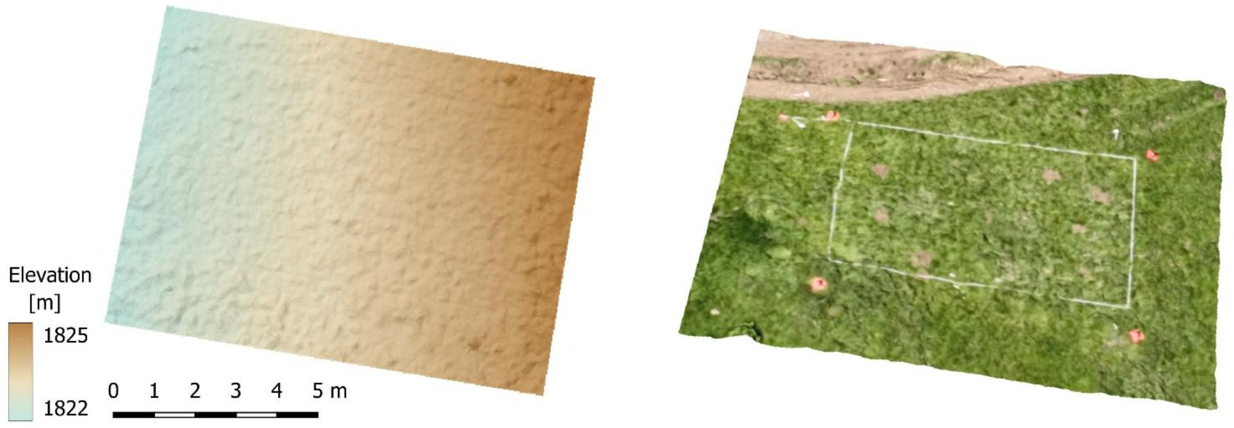
The UAV survey resulted in two georeferenced datasets: the DTM and orthophoto mosaic of the habitat in two separate GeoTIFF files with 0.025 m/pixel spatial resolution. Both are able to capture the spatial pattern of burrow mounds at centimetre-scale resolution (horizontally). Later, the specific area surveyed by GPR was clipped from both datasets, and it was saved as a textured 3D model in *.OBJ format (Figure 3).

3.2. GPR Imaging and Dataset

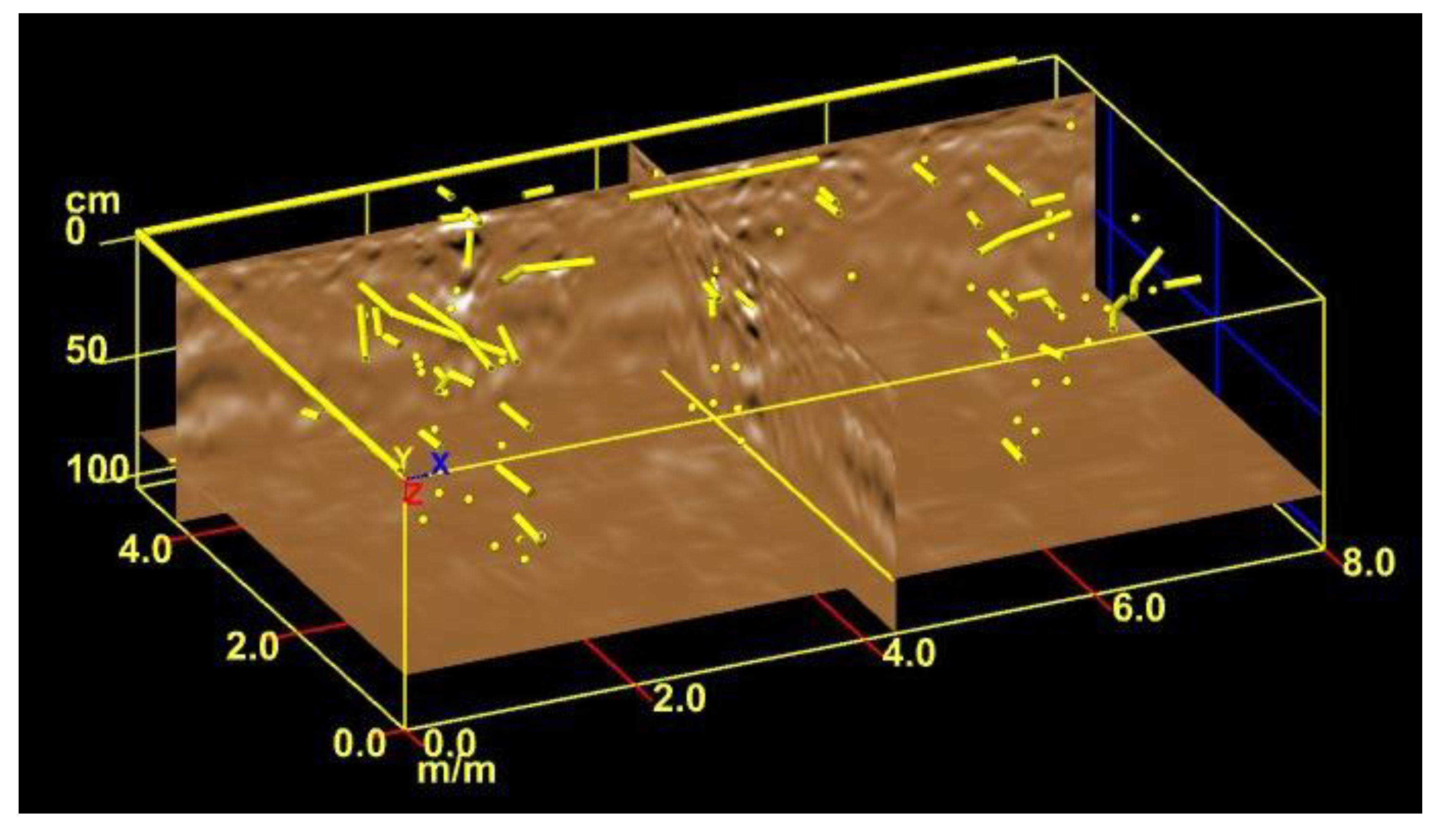
The GPR survey yielded a 3D radar volume exported as a *.DXF file, containing the interpreted positions, which are interpretative or exploratory reconstructions rather than a validated representation of the burrow system, of subsurface burrow segments (vertically) (Figure 4), together with manually digitised lines indicating the rectangular cuboid of the surveyed sampling site.

Although the GPR system (GSSI SIR-4000) recorded standard GPS positions for each trace in the raw *.DZG data file, those locations included significant horizontal or vertical inaccuracies of about 0.5 m on average. As a result of this inaccuracy, we used a local coordinate system underground as well as on the surface. This procedure replaced the lower-precision GPS positions with locally accurate coordinates, while maintaining the relative position of both surface and subsurface objects and data points (locations) (Figure 4).

3.3. Workflow for Integrating UAV and GPR Datasets

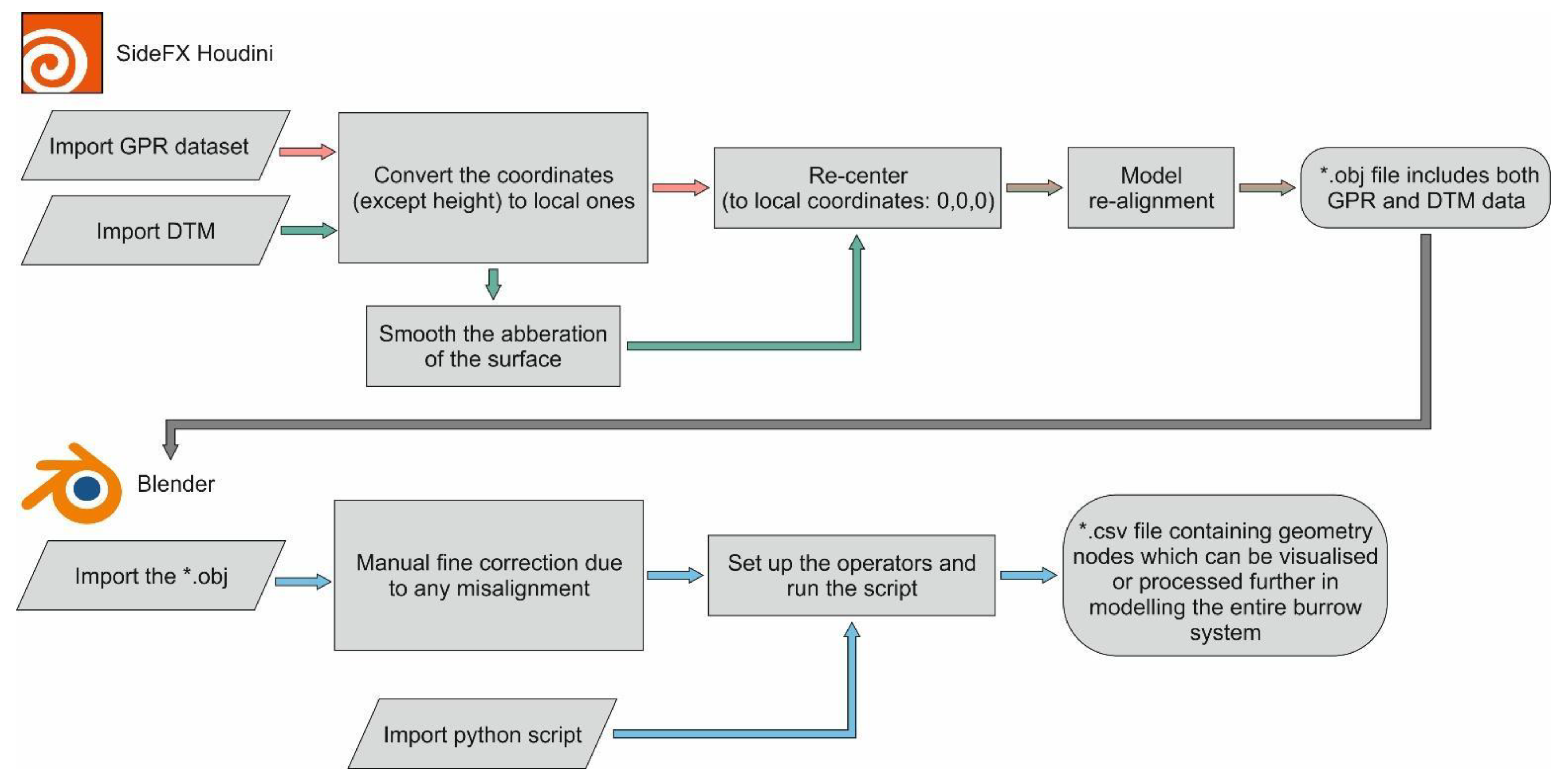
The processing workflow successfully showed how UAV-derived surface models, DTM, and GPR-derived subsurface volumes originating in different coordinate reference systems and formats can be integrated using freely available software tools. Figure 5. displays the various steps of processing the original files and provides a detailed workflow from data collection to the generation of a joint 3D voxelised dataset.

SideFx Houdini software is much more configurable, and unlike Blender, it does not require the creation of a complex node tree during projection transformation. However, voxelization is easier to perform in Blender, as it uses standard Python interpretations, while Houdini often uses special interpretations in its code that are specific to the software.

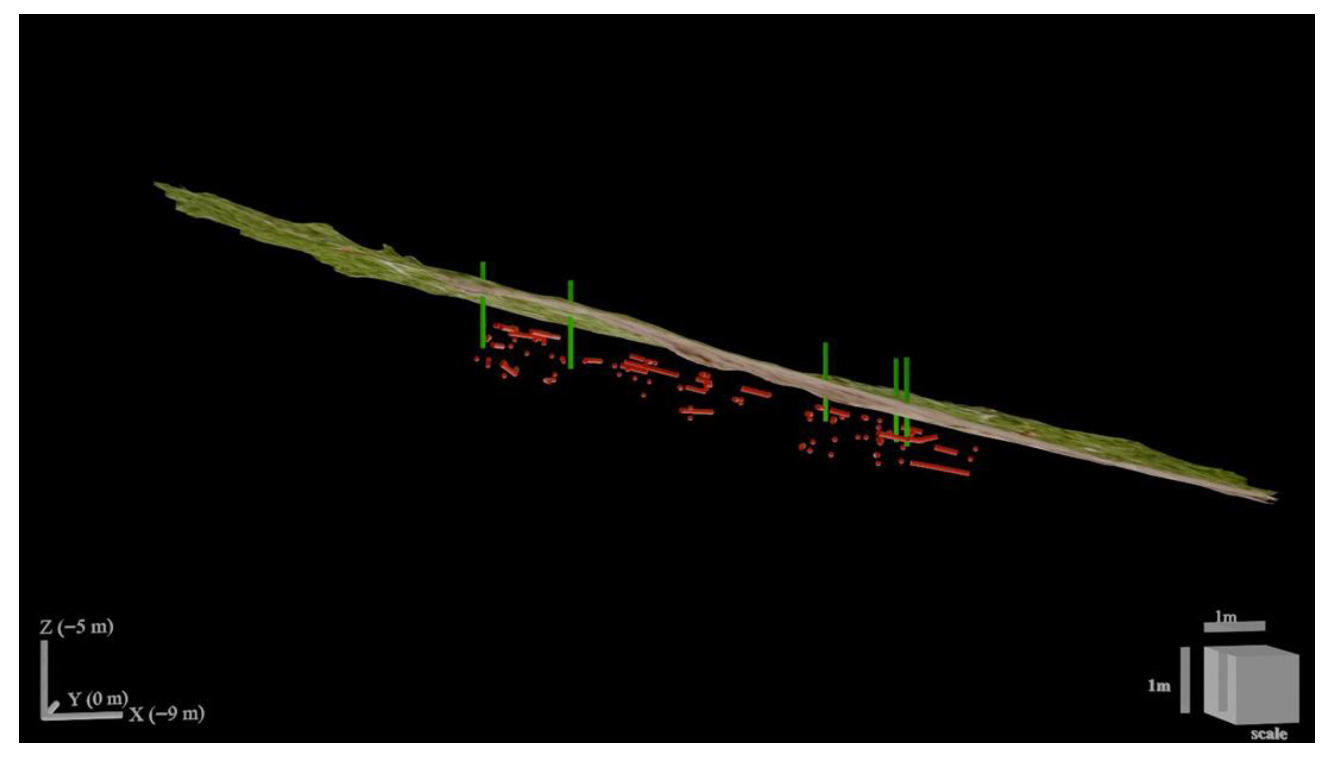
After format conversion to a common format, *.OBJ, both datasets were imported into SideFX Houdini, where coordinate-system harmonisation and alignment were performed manually using the common control points of both datasets. The upper corners of the cuboid were used both horizontally and vertically, as they are represented in the textured DTM: horizontally as lines in the texture as rulers lying on the ground, and vertically as the surface of the generated DTM. The alignment error of this fine registration resulted in increased horizontal and vertical positional accuracy within ±0.02 m (horizontal) and ±0.03 m (vertically) due to the small size of the test site and the internal rigidity of the two datasets. Additionally, this error is below the average diameter of the burrows; therefore, the complex dataset is suitable for any subsequent processing steps and modelling. Furthermore, it resulted in the correct alignment of GPR line scans in the 3D grid and the surface area within that grid, including burrow mounds and other terrain features. That correctional step was necessary to amalgamate the 3D surface texture, DTM, with the subsurface 3D burrows and volume (Figure 6). Additionally, joining the precise mound locations, which represent vertical burrow sections, to the subsurface burrow sections results in a more accurate and descriptive dataset for the subsequent voxelisation step.

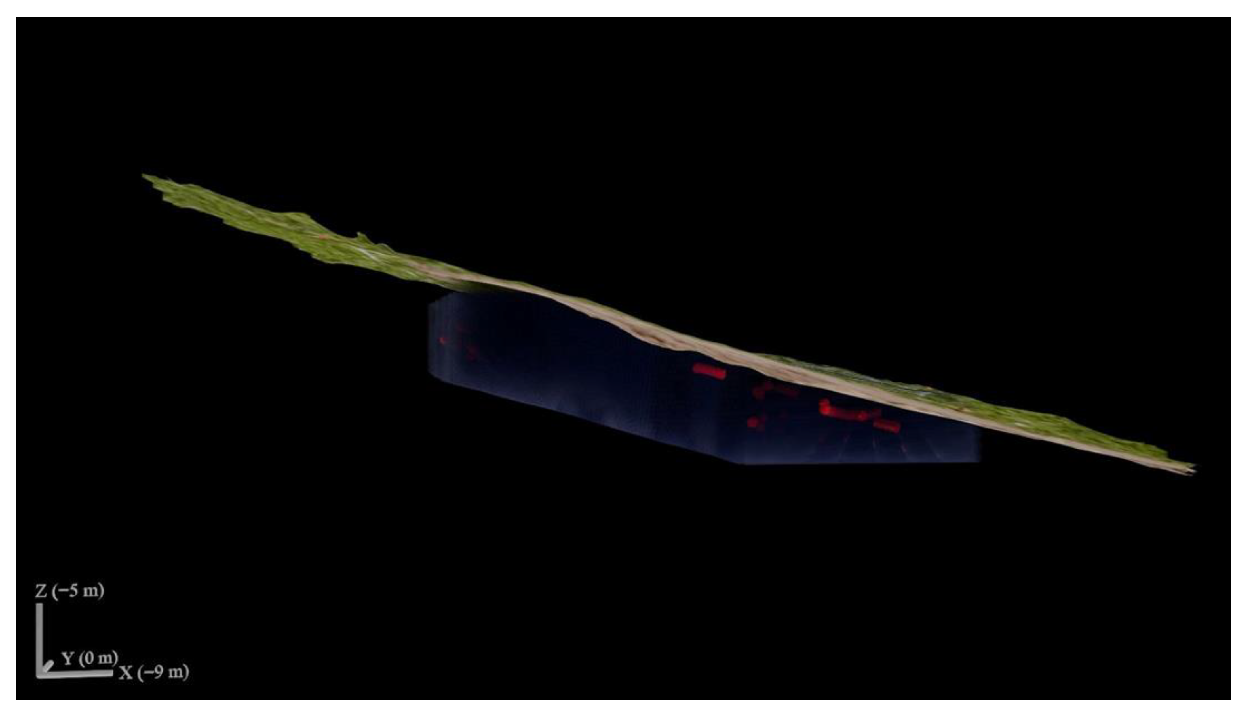
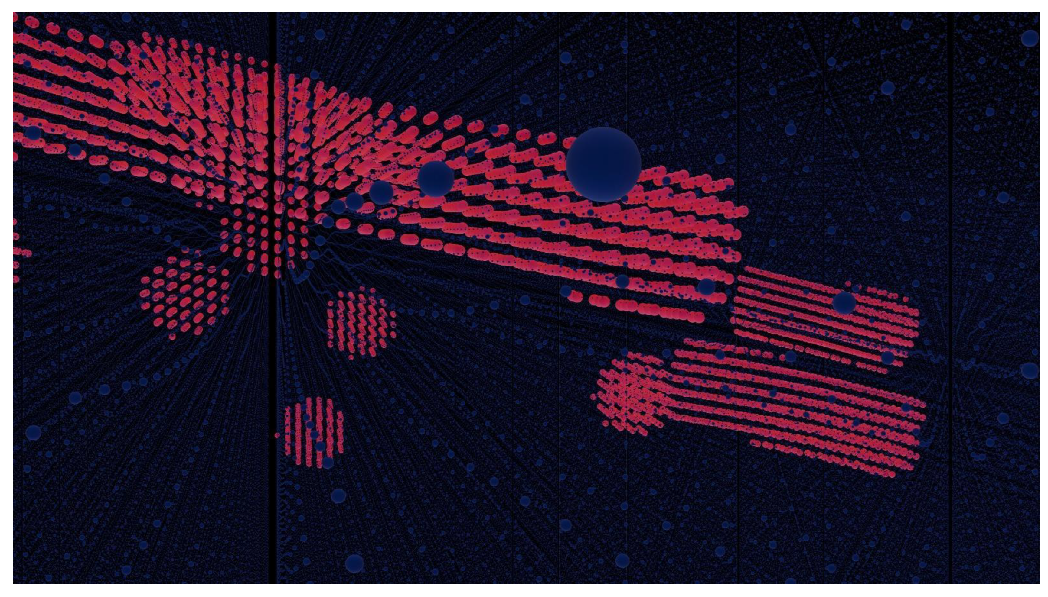
Finally, the aligned composite OBJ was processed in Blender, where subsurface burrow segments from the GPR volume were inserted into the combined point cloud. The images from this processing (Figure 7 and Figure 8) show this voxelisation step, in which the integrated body was discretised into a structured 3D body, indicating the presence of the burrow in a voxel as “1” (including the burrow opening on the surface). The final 3D dataset containing voxels displays the spatial overlap between UAV-derived mounds and GPR-derived burrows. This simplified format, in which voxels had either 0 or 1 score, enabled further modelling or assessment of how surface mounds, including burrow openings, corresponded to subsurface architecture. In the course of the experiment, calculations were conducted using burrows with a diameter of 0.07 m. The script generated 7,730,587 voxels in the cuboid, of which 48,952 have a value of 1, indicating burrows. The voxels with a mask value of 1 represent all burrows that were marked during the GPR survey.

3.4. Voxelised Output

The 3D body containing the subsurface architecture as 1 s and 0 s was then exported as a *.CSV file containing the following information:

(1)

(x, y, z) voxel centroid coordinates;

(2)

“1” for voxels containing subsurface burrow segments, “0” otherwise.

Those pieces of information enable a georeferenced 3D representation of segments of the burrow system, suitable for quantitative spatial analyses and modelling. The presented workflow resulted in a single 3D body containing voxels and numerical, binary information within it, providing a common, simple format for further processing. The whole processing from datasets collected by specialised tools used only freely available software.

4. Discussion

4.1. Possible Limits of the GPR Survey and Interpretation

GPR-based detection of small animal burrows is strongly influenced by local soil conditions. High electrical conductivity, typically associated with clay-rich, saline, or water-saturated soils, attenuates radar signals and reduces penetration depth, making small voids difficult to identify. Moreover, soil strongly mixed with gravel, stones, or dense plant roots can cause scattering of wave signals, which can distort and obscure the characteristic hyperbolic reflections of air-filled burrows. High moisture content and the gradient between different horizons can further distort signal travel times and complicate interpretation. The combination of these factors can reduce the contrast between the burrow and the surrounding soil, increasing the likelihood of false negatives or positives, and, as a result, limiting the reliability of GPR surveys. Consequently, it is recommended that practitioners validate the interpretation of the GPR analysis by quantitative accuracy metrics.

Studies describing animal burrows usually lack quantitative information on burrow structure, such as length, number of curves, and maps of burrow systems. For the Nannospalax leucodon species complex, the literature on their burrows is even rarer [38,47,48]. Our approach of using various non-destructive, proximal sensing tools and 3D-modelling methods could give a way to go beyond these rather anecdotal, variable descriptions by demonstrating a methodology that enables the estimation of quantitative geometric characteristics if the GPR findings are authentically verified by means of excavation or through targeted subsurface sampling schemes, during which the locations of the GPR-predicted burrows were confirmed.

4.2. Benefits of a Unified, Open-Source Workflow

The workflow presented here illustrates the feasibility and reproducibility of integrating different datasets using free, open-source platforms, such as Blender, CloudCompare, QGIS (an open-source alternative to ArcGIS), and Houdini. Freely available software provides a methodology for wider public dissemination yet enables control over different steps during processing, such as coordinate transformation, point cloud or mesh manipulation, 3D-body or volume reconstruction, and user-friendly visualisation. In other words, this workflow and file processing from data collection to visualisation create a toolbox to be used for studying animal-built structures or similar shallow subsurface phenomena.

In particular, the final, unified 3D-body of the surface and subsurface structures of the burrow system, the voxelised volume with binary, 0 or 1, values within the voxels, could provide a common way to analyse burrow or underground structures quantitatively, including both observed and inferred parts, and process them further in spatial modelling.

The final product of combining and processing different spatial datasets is a common *.CSV file. As a result of this text format’s general usage and compatibility with other programmes and applications, it can easily be input into advanced modelling procedures. For instance, a planned and possible follow-up work could include adding covariates and/or auxiliary variables to the model applied, such as terrain reflecting microtopography, soil characteristics, surface vegetation patterns, spatial regularities, etc., to model the hidden segments of the burrow system with higher accuracy and precision if GPR data was validated at the beginning of the study by means of excavation or verified sampling from burrows by, for example, core samplers. Future analyses will apply spatial modelling and stochastic simulation to estimate the probability of burrow presence in unobserved voxels. These modelling approaches will produce uncertainty quantification, allowing the construction of probabilistic realisations of the complete burrow network. The unified dataset generated in the current study is thus an essential precursor to predictive reconstruction of hidden burrow structures.

The voxelization process is planned to be extended to the surface, which connects identifiable burrow openings on the surface with passages detected below the surface. The method of voxelisation used for the surface DTM would be similar to the voxelisation process presented in this study for the underground volume, i.e., a voxel would be created from the surface to a certain height, where a value of 0 would indicate points where there is no possible burrow entrance, and a value of 1 would indicate there is a potential burrow entrance on the surface. This approach could provide a common method to combine measurements both above and below ground.

Another important aspect of our results is that it shows how merging UAV and GPR data in a common inertia system gives new insight into the relationship between surface patterns, such as mounds, and 3D geometry of subsurface objects, such as burrows. This can further support various studies or help to answer questions that are related to soil disturbance and its spatio-temporal dynamics, burrowing behaviour, and habitat (subsurface) engineering by burrowing mammals.

The current methodology’s and workflow’s (Figure 5) novelty compared with previous studies lies within the combination of different proximal sensing techniques and freely available 3D software that can harmonise and align coordinate systems. Those techniques, including Blender and Houdini software, and UAV and GPR tools, provide procedural environments that can handle data coming from both UAVs and GPRs and can overcome limitations of separate, costly multi-software 3D workflows. The combined usage of the software upon data acquisition can involve modelling and rendering of spatial data. Usage of these platforms integrates modelling and rendering spatial data into a single pipeline, reducing data transfers and improving reproducibility. Their node-based systems enable rule-driven, parameterised construction of complex structures like animal burrows, supporting rapid iteration and data-driven modelling. Moreover, they offer support for volumetric data, cross-sections, and layered rendering, allowing clear visualisation of internal structures that is difficult to achieve with only surface- or subsurface-focused methods. By joining surface and subsurface images, visualisation or further 3D modelling of the unified dataset becomes feasible.

Nevertheless, it should be noted that despite the advantages of binarisation, such as the removal of noise and reflections of objects of no interest, it has disadvantages, such as the removal of information about signal strength and interpretation confidence. By generating the voxels after applying a consistent interpretation criterion across orthogonal profiles and removal of ambiguous reflections lacking cross-profile continuity, we were able to mitigate this disadvantage. As a result, the voxelised cuboid can be viewed as a distilled representation of interpreted burrow structures and not as a substitute for the full GPR dataset with reflection amplitude or intensity.

5. Conclusions

This study presents a reproducible, open-source workflow and protocol for integrating UAV-derived surface data and GPR-derived subsurface information into a unified 3D voxel-based model of animal burrows. By combining data originally stored in different coordinate systems (UTM and WGS84) and formats (GeoTIFF, DXF) and processing them through freely available software (Houdini and Blender), we demonstrate a flexible pipeline capable of harmonising and visualising complex multisensory datasets. The final voxelised product retains explicit spatial coordinates and binary occupancy values, enabling quantitative assessments of subsurface burrow architecture in relation to surface mound morphology. Nevertheless, the inability to validate the GPR results in the field means that the findings represent interpreted geophysical anomalies rather than verified spatial geometry of the burrow system. Consequently, the main aim was to demonstrate the combined application of different tools and approaches to meet those aims. Due to various reasons, including the remote study area in the Albanian mountains, the lack of relevant and published publications on burrow morphology of Lesser mole rats and the protection of this species (or species complex) in countries, we were unable to verify or validate our partial burrow model. However, this was just a part of the results contributing to the workflow of how we have come to the complete 3D object of surface and subsurface data and a simple *.CSV data format containing information on the exact location of burrows. Nevertheless, the location and spatial relationship of surface burrow openings (Figure 6) and underground burrow segments visually illustrate that virtual and visual images of burrow openings extended into the subsurface and crossed the underground burrow segments, which provides partial validation of the underground burrows, indicating their real presence.

Overall, at the technical level of our research study, we were unable to verify the validity of the reconstruction, but further work could build up the 3D structure of animal burrows, and if it is planned preliminarily, that structure could be verified and its accuracy determined quantitatively.

The workflow provides an essential foundation for subsequent spatial modelling efforts. The voxelised dataset produced here will serve as the core input for probabilistic reconstruction of unseen burrow segments using statistical approaches, incorporating environmental covariates and enabling uncertainty estimation. As such, the present work contributes both a methodological framework and a data integration strategy that can support a wide range of geomatics applications where surface–subsurface coupling is essential. This approach holds promise for ecological, archaeological, and engineering investigations requiring the joint analysis of topographic and subsurface geophysical observations.

References

1. Lindtner, P.; Svitok, M.; Ujházy, K.; Kubovčík, V. Disturbances by the European Ground Squirrel Enhance Diversity and Spatial Heterogeneity of Plant Communities in Temperate Grassland. Biodivers. Conserv. 2020, 29, 853–867. [Google Scholar] [CrossRef]
2. Newediuk, L.J.; Hare, J.F. Burrowing Richardson’s Ground Squirrels Affect Plant Seedling Assemblages via Environmental but Not Seed Bank Changes. Curr. Zool. 2020, 66, 219–226. [Google Scholar] [CrossRef]
3. Ligthart, T.N.; Peek, G.J.W.C.; Taber, E.J. A Method for the Three-Dimensional Mapping of Earthworm Burrow Systems. Geoderma 1993, 57, 129–141. [Google Scholar] [CrossRef]
4. Walker, L.R.; Vrooman, S.S.; Thompson, D.B. Rodent Mounds Facilitate Shrubs and Shrubs Inhibit Seedlings in the Mojave Desert, USA. J. Arid Environ. 2015, 113, 95–101. [Google Scholar] [CrossRef]
5. Gabet, E.J.; Reichman, O.J.; Seabloom, E.W. The Effects of Bioturbation on Soil Processes and Sediment Transport. Annu. Rev. Earth Planet. Sci. 2003, 31, 249–273. [Google Scholar] [CrossRef]
6. Wilkinson, M.T.; Richards, P.J.; Humphreys, G.S. Breaking Ground: Pedological, Geological, and Ecological Implications of Soil Bioturbation. Earth. Sci. Rev. 2009, 97, 257–272. [Google Scholar] [CrossRef]
7. Haussmann, N.S. Soil Movement by Burrowing Mammals: A Review Comparing Excavation Size and Rate to Body Mass of Excavators. Prog. Phys. Geogr. 2017, 41, 29–45. [Google Scholar] [CrossRef]
8. Németh, A.; Mizsei, E.; Laczkó, L.; Czabán, D.; Hegyeli, Z.; Lengyel, S.; Csorba, G.; Sramkó, G. Evolutionary History and Systematics of European Blind Mole Rats (Rodentia: Spalacidae: Nannospalax): Multilocus Phylogeny and Species Delimitation in a Puzzling Group. Mol. Phylogenet. Evol. 2024, 190, 107958. [Google Scholar] [CrossRef] [PubMed]
9. White, T.A.; Lundy, M.G.; Montgomery, W.I.; Montgomery, S.; Perkins, S.E.; Lawton, C.; Meehan, J.M.; Hayden, T.J.; Heckel, G.; Reid, N.; et al. Range Expansion in an Invasive Small Mammal: Influence of Life-History and Habitat Quality. Biol. Invasions 2012, 14, 2203–2215. [Google Scholar] [CrossRef]
10. Krebs, C.J. Population Fluctuations in Rodents; University of Chicago Press: Chicago, IL, USA, 2013; ISBN 9780226010496. [Google Scholar]
11. Williams, J.J.; Freeman, R.; Spooner, F.; Newbold, T. Vertebrate Population Trends Are Influenced by Interactions between Land Use, Climatic Position, Habitat Loss and Climate Change. Glob. Change Biol. 2022, 28, 797–815. [Google Scholar] [CrossRef]
12. Lan, B.L.; Chandran, P. Distribution of Animal Population Fluctuations. Phys. A Stat. Mech. Appl. 2011, 390, 1289–1294. [Google Scholar] [CrossRef]
13. Gedeon, C.I.; Árvai, M.; Szatmári, G.; Brevik, E.C.; Takáts, T.; Kovács, Z.A.; Mészáros, J. Identification and Counting of European Souslik Burrows from UAV Images by Pixel-Based Image Analysis and Random Forest Classification: A Simple, Semi-Automated, yet Accurate Method for Estimating Population Size. Remote Sens. 2022, 14, 2025. [Google Scholar] [CrossRef]
14. Šumbera, R.; Mazoch, V.; Patzenhauerová, H.; Lövy, M.; Šklíba, J.; Bryja, J.; Burda, H. Burrow Architecture, Family Composition and Habitat Characteristics of the Largest Social African Mole-Rat: The Giant Mole-Rat Constructs Really Giant Burrow Systems. Acta Theriol. 2012, 57, 121–130. [Google Scholar] [CrossRef]
15. Meadows, A. Burrows and Burrowing Animals: An Overview. In The Environmental Impact of Burrowing Animals and Animal Burrows; Meadows, P.S., Meadows, A., Eds.; Clarendon Press: Oxford, UK, 1991; pp. 1–13. [Google Scholar]
16. Erfanifard, Y.; Kraszewski, B.; Stereńczak, K. Integration of Remote Sensing in Spatial Ecology: Assessing the Interspecific Interactions of Two Plant Species in a Semi-Arid Woodland Using Unmanned Aerial Vehicle (UAV) Photogrammetric Data. Oecologia 2021, 196, 115–130. [Google Scholar] [CrossRef]
17. Kellenberger, B.; Veen, T.; Folmer, E.; Tuia, D. 21 000 Birds in 4.5 H: Efficient Large-Scale Seabird Detection with Machine Learning. Remote Sens. Ecol. Conserv. 2021, 7, 445–460. [Google Scholar] [CrossRef]
18. Wu, W.; Liu, S.; Zhong, X.; Liu, X.; Wang, D.; Lin, K. Brandt’s Vole Hole Detection and Counting Method Based on Deep Learning and Unmanned Aircraft System. Front. Plant Sci. 2024, 15, 1290845. [Google Scholar] [CrossRef]
19. Stuhler, J.D.; Portillo-Quintero, C.; Goetze, J.R.; Stevens, R.D. Efficacy of Remote Sensing Technologies for Burrow Count Estimates of a Rare Kangaroo Rat. Wildl. Soc. Bull. 2024, 48, e1510. [Google Scholar] [CrossRef]
20. Kearney, S.P.; Porensky, L.M.; Augustine, D.J.; Pellatz, D.W. Toward Broad-Scale Mapping and Characterization of Prairie Dog Colonies from Airborne Imagery Using Deep Learning. Ecol. Indic. 2023, 154, 110684. [Google Scholar] [CrossRef]
21. Dojack, L. Ground Penetrating Radar Theory, Data Collection, Processing, and Interpretation: A Guide for Archaeologists; University of British Columbia, Laboratory of Archaeology: Vancouver, BC, Canada, 2012. [Google Scholar] [CrossRef]
22. Jol, H.M. (Ed.) Ground Penetrating Radar Theory and Applications, 1st ed.; Elsevier: Amsterdam, The Netherlands, 2009; ISBN 978-0-444-53348-7. [Google Scholar]
23. Iftimie, N.; Savin, A.; Steigmann, R.; Dobrescu, G.S. Underground Pipeline Identification into a Non-Destructive Case Study Based on Ground-Penetrating Radar Imaging. Remote Sens. 2021, 13, 3494. [Google Scholar] [CrossRef]
24. Sherrod, L.; Sauck, W.; Simpson, E.; Werkema, D.; Swiontek, J. Case Histories of GPR for Animal Burrows Mapping and Geometry. J. Environ. Eng. Geophys. 2019, 24, 1–17. [Google Scholar] [CrossRef]
25. Agrafiotis, P.; Lampropoulos, K.; Georgopoulos, A.; Moropoulou, A. 3D Modelling the Invisible Using Ground Penetrating Radar. Int. Arch. Photogramm. Remote Sens. Spat. Inf. Sci. ISPRS Arch. 2017, 42, 33–37. [Google Scholar] [CrossRef]
26. Zhang, C.; Gravey, M.; Mariéthoz, G.; Irving, J. Reconstruction of High-Resolution 3D GPR Data from 2D Profiles: A Multiple-Point Statistical Approach. Remote Sens. 2024, 16, 2084. [Google Scholar] [CrossRef]
27. Rowaizak, M.; Farhat, A.; Khalil, R. From Brain Lobes to Neurons: Navigating the Brain Using Advanced 3D Modeling and Visualization Tools. J. Imaging 2025, 11, 298. [Google Scholar] [CrossRef]
28. SideFX SideFX Houdini for Windows 2026. Available online: https://www.sidefx.com/ (accessed on 17 November 2025).
29. Naiman, J.P.; Borkiewicz, K.; Christensen, A.J. Houdini for Astrophysical Visualization. Publ. Astron. Soc. Pac. 2017, 129, 58008. [Google Scholar] [CrossRef]
30. Ueda, K. From Craft to Code and Back: Biodegradable Polyester, Institutional Co-Design, and Garment Practice in Nishijin Weaving. Arts 2026, 15, 34. [Google Scholar] [CrossRef]
31. McLennan, S.; Brown, A. A Smart Heritage System to Re-Generate New Zealand’s 19th Century Timber Churches. Heritage 2021, 4, 4040–4055. [Google Scholar] [CrossRef]
32. Evgeniya, S. Designing and Building a Three-Dimensional Environment Using Blender 3D and Unity Game Engine. Bachelor’s Thesis, Univesity of Applied Sciences, Lapland, Finland, 2016. [Google Scholar]
33. Romilio, A.; Murphey, P.C.; Matthews, N.A.; Schumacher, B.A.; Murphey, L.D.; Toscanini, M.; Boyce, P.; Fitzner, Z. Track by Track: Revealing Sauropod Turning and Lateralised Gait at the West Gold Hill Dinosaur Tracksite (Upper Jurassic, Bluff Sandstone, Colorado). Geomatics 2025, 5, 67. [Google Scholar] [CrossRef]
34. Romilio, A.; Shao, C. Analysing Trackway-Based Speed Calculations to Infer Dinosaur Locomotive Capabilities and Behaviours. Hist. Biol. 2024, 36, 2244–2253. [Google Scholar] [CrossRef]
35. Romilio, A.; Park, R.; Nichols, W.; Jackson, O. Dinosaur Footprints from the Lower Jurassic (Hettangian–Sinemurian) Precipice Sandstone of the Callide Basin, Queensland, Australia. Hist. Biol. 2026, 38, 134–145. [Google Scholar] [CrossRef]
36. Romilio, A. Blender as a Tool for Palaeoichnological Research: Case Study from Lark Quarry. Geobios 2025, 88–89, 219–226. [Google Scholar] [CrossRef]
37. Bego, F.; Loçe, E.; Topoviti, D. First Record of the Lesser Mole Rat (Spalax Leucodon, Nordmann, 1840) in Albania: Updated List of Small Terrestrial Mammals. Universi–Int. J. Educ. Sci. Technol. Innov. Health Environ. 2014, 1, 10–15. [Google Scholar]
38. Šklíba, J.; Lövy, M.; Koeppen, S.C.W.; Pleštilová, L.; Vitámvás, M.; Nevo, E.; Šumbera, R. Activity of Free-Living Subterranean Blind Mole Rats Spalax Galili (Rodentia: Spalacidae) in an Area of Supposed Sympatric Speciation. Biol. J. Linn. Soc. 2016, 118, 280–291. [Google Scholar] [CrossRef]
39. Niu, L.; Wang, Z.; Lin, Z.; Zhang, Y.; Yan, Y.; He, Z. Voxel-Based Navigation: A Systematic Review of Techniques, Applications, and Challenges. ISPRS Int. J. Geoinf. 2024, 13, 461. [Google Scholar] [CrossRef]
40. Madoš, B.; Balaz, A.; Adám, N.; Hurtuk, J. Information Hiding into OBJ Format File Using Vector Steganography Techniques. In Proceedings of the 2018 IEEE 12th International Symposium on Applied Computational Intelligence and Informatics (SACI), Timișoara, Romania, 17–19 May 2018; pp. 91–96. [Google Scholar] [CrossRef]
41. Čapek, D.; Petřík, M.; Pachman, J.; Watson, E.; Haloda, J.; Macke, R.; Henych, T.; Koten, P.; Schimmerohn, M.; Stravová, Z.; et al. 3D Shape Models for Describing Monolithic Asteroids and Meteoroids. Astron. Astrophys. 2025, 696, A40. [Google Scholar] [CrossRef]
42. Praschl, C.; Krauss, O. Extending 3D Geometric File Formats for Geospatial Applications. Appl. Geomat. 2024, 16, 161–180. [Google Scholar] [CrossRef]
43. Kato, A.; Ohno, N. Construction of Three-Dimensional Tooth Model by Micro-Computed Tomography and Application for Data Sharing. Clin. Oral Investig. 2009, 13, 43–46. [Google Scholar] [CrossRef] [PubMed]
44. Janssen, P.; Chen, K.W.; Basol, C. Iterative Virtual Prototyping: Performance Based Design Exploration. In Proceedings of the International Conference on Education and Research in Computer Aided Architectural Design in Europe; Zupancic, T., Juvancic, M., Verovsek, S., Jutraz, A., Eds.; eCAADe: Brussels, Belgium, 2011; pp. 253–260. [Google Scholar]
45. De Lima, R.R.; Carvalho, L.R.R.A. 3D Printing for Advanced Surgical Planning in Veterinary Medicine—Case Studies, Methods and Future Perspectives. Front. Vet. Sci. 2025, 12, 1596577. [Google Scholar] [CrossRef]
46. Hess, R. Blender Foundations: The Essential Guide to Learning Blender 2.6; Routledge: London, UK, 2013; pp. 1–404. [Google Scholar] [CrossRef]
47. Yağcı, T.; Aşan, N.; Coşkun, Y. The Tunnel Structure of Blind Mole Rats (Genus Spalax) in Turkey: (Rodentia: Spalacidae). Zool. Middle East 2010, 50, 35–40. [Google Scholar] [CrossRef]
48. Thomas, H.G.; Bateman, P.W.; Le Comber, S.C.; Bennett, N.C.; Elwood, R.W.; Scantlebury, M. Burrow Architecture and Digging Activity in the Cape Dune Mole Rat. J. Zool. 2009, 279, 277–284. [Google Scholar] [CrossRef]
Figure 1. Location and study site of the surveys. A mole-rat and a mound built during their underground activity are shown for illustration and easier imagination of the focal objects and species.
Geomatics 06 00048 g001
Figure 2. Survey design of the 3D grid (8 × 5 m) for the GPR. During the unidirectional survey, 47 GPR profiles were collected at the speed of <~1 m*s−1, a slow walking speed.
Geomatics 06 00048 g002
Figure 3. UAV-derived digital terrain model (left) and texturised 3D model (right). The figure shows surface features, including mounds that cover burrow openings.
Geomatics 06 00048 g003
Figure 4. The 3D GPR radar volume exported from RADAN 7 as a 3D *.DXF file. The “tubes” show the segments of the burrows. The corrected GPR volume shows improved continuity and a regulated pattern after coordinate correction, which enables integration with the 3D texture of the surface.
Geomatics 06 00048 g004
Figure 5. This figure gives an overview of the workflow from UAV and GPR data import to voxelisation of the final 3D image. Arrows between boxes or steps indicate data flow between acquisition systems, software environments, and output formats.
Geomatics 06 00048 g005
Figure 6. Both UAV and GPR datasets were converted into OBJ formats to be imported into SideFX Houdini. The figure shows the UAV surface mesh and GPR subsurface geometry after reprojection into a shared local coordinate system. The green vertical tubes indicate the positions of surface mounds (the length of the green tubes is not to scale), and the red tubes indicate the burrows. Created in Blender.
Geomatics 06 00048 g006
Figure 7. A merged *.OBJ geometry loaded into Blender, which shows the unified point cloud. The point cloud is divided into discrete voxels, and each voxel is classified into voxels that contain burrow parts (“1”) or anything else (“0”). The blue voxels have a mask value of 0, and the red voxels have a mask value of 1. Created in Blender.
Geomatics 06 00048 g007
Figure 8. Close-up image of the voxels. Blue voxels represent the mask value of 0, and red voxels represent the mask value of 1. Created in Blender.
Geomatics 06 00048 g008
Disclaimer/Publisher’s Note: The statements, opinions and data contained in all publications are solely those of the individual author(s) and contributor(s) and not of MDPI and/or the editor(s). MDPI and/or the editor(s) disclaim responsibility for any injury to people or property resulting from any ideas, methods, instructions or products referred to in the content.