Article

Assessing PlanetScope Imagery for Satellite-Derived Bathymetry Using ICESat-2 ATL03 Photon-Based Validation: A Case Study at Cayo Alburquerque, Caribbean Colombia


by
Jose Eduardo Fuentes Delgado
AGESAT Research Group (Grupo de Investigación Análisis y Gestión para la Sostenibilidad Ambiental y Territorial), Department of Geography, Universidad del Valle, Cali 760031, Colombia
Geomatics 2026, 6(2), 39; https://doi.org/10.3390/geomatics6020039
Submission received: 9 March 2026 / Revised: 14 April 2026 / Accepted: 15 April 2026 / Published: 20 April 2026

Highlights

What are the main findings?
  • We develop a reproducible, end-to-end PlanetScope (8-band, 3 m) SDB workflow that uses ICESat-2 ATL03 seafloor photons as independent vertical control; after quality assurance and quality control (QA/QC), refraction correction, and water masking, 5021 co-located control points support calibration and validation at the reef scale.
  • At Cayo Alburquerque, multiband models outperform the log-ratio approach; Lyzenga provides the best performance and stability across splits (R2 = 0.843 to 0.859; RMSE = 1.734 to 1.813 m), followed by Bierwirth, whereas Stumpf is unsuitable under the evaluated optical conditions.
What are the implications of the main findings?
  • ICESat-2 photons provide scalable, independent vertical control where echo sounding is unavailable, but they are not hydrographic-grade; photon classification, refraction, sea state, and spatial-support mismatch can introduce decimeter-to-meter uncertainties that should be reported when ranking SDB models.
  • Lyzenga 2006 is recommended as an operational baseline for scalable reef SDB, provided that sun-glint correction and refraction correction are applied, calibration is depth-balanced, and uncertainty and domain-of-applicability constraints are explicitly reported.

Abstract
Satellite-derived bathymetry (SDB) offers a practical alternative for mapping shallow reefs in remote oceanic settings where acoustic surveys are costly and logistically constrained. Here we benchmark PlanetScope 8-band (3 m) surface reflectance—an underused commercial constellation for reef SDB—using ICESat-2 Advanced Topographic Laser Altimeter System (ATLAS) ATL03 photon data (Release 006) as independent vertical control. Seventeen ATL03 ground tracks (2019–2025) were processed using geometric filtering, photon classification, and explicit air–water refraction correction. This yielded 5171 candidate seafloor observations, of which 5021 were co-located with valid PlanetScope water pixels after Usable Data Mask screening (UDM2/UDM2.1), sun-glint correction, and reflectance quality screening. Four SDB formulations (Lyzenga, Bierwirth, and Stumpf) were calibrated and independently validated using depth-stratified train/validation partitions (70/30, 80/20, and 90/10). Across partitions, the multiband polynomial model of Lyzenga 2006 generalized best (R2 = 0.843–0.859; RMSE = 1.734–1.813 m; bias = −0.070 to −0.081 m), followed by Bierwirth (R2 = 0.826–0.845; RMSE = 1.818–1.904 m). Lyzenga 1985 reported lower skill (RMSE ≈ 3.1 m), while the Stumpf log-ratio failed in independent validation. ICESat-2 photon bathymetry provides repeatable point-based control in clear waters but remains less precise than echo sounding due to photon classification and spatial-support effects; therefore, uncertainties and applicability limits must be reported. Overall, PlanetScope 3 m, 8-band surface reflectance supports reproducible reef-scale SDB in Seaflower under the evaluated conditions, with Lyzenga 2006 as a robust baseline.

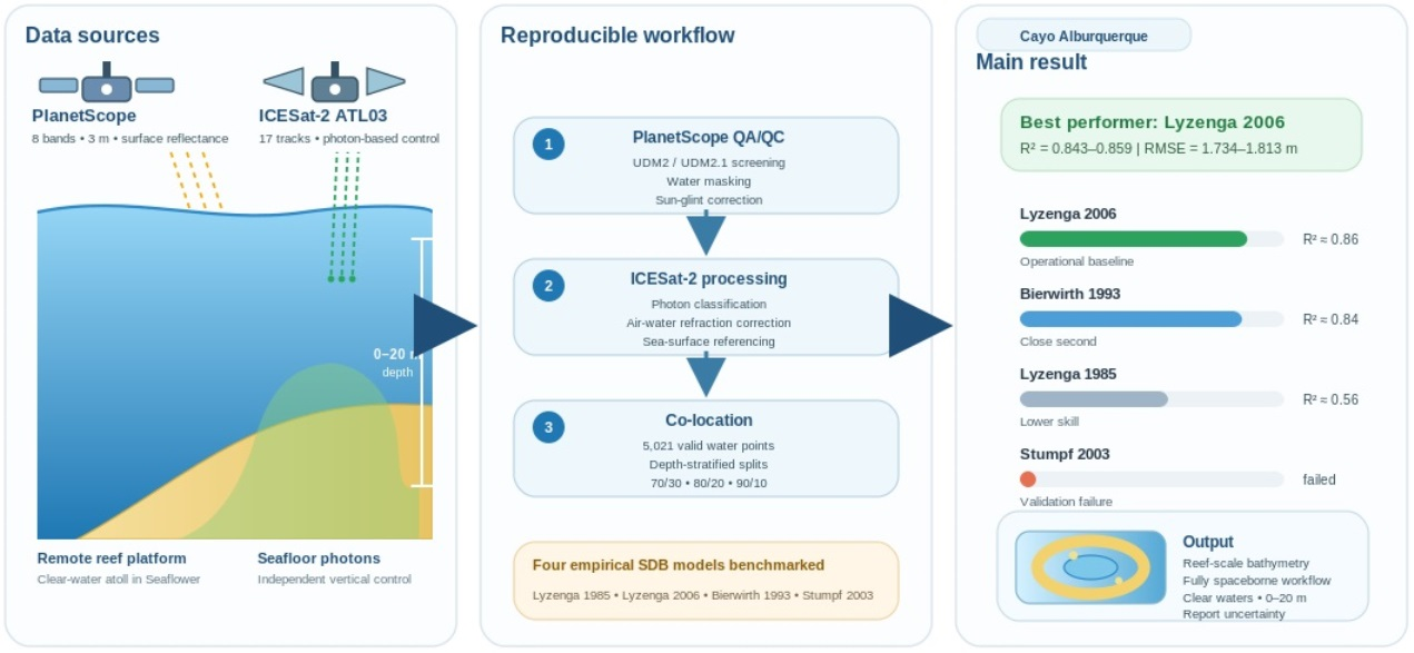
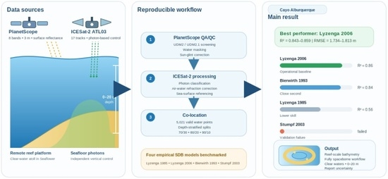
Graphical Abstract

1. Introduction

Bathymetric mapping is a cross-cutting and critical input for safe navigation, coastal planning, conservation of strategic ecosystems, and hydrodynamic modeling. Despite its importance, more than 50% of global coastal areas are estimated to lack detailed bathymetric information, which constrains informed decision-making and the generation of derived products [1]. In remote insular regions such as the Archipelago of San Andres, Providencia, and Santa Catalina in Colombia, data acquisition using conventional methods (single beam or multibeam echo sounding and airborne Light Detection and Ranging (LiDAR)) faces significant logistical constraints and prohibitive operating costs. As a result, information gaps persist in areas of high environmental vulnerability and strategic value for ecological management and spatial planning. In this context, satellite-derived bathymetry (SDB) has emerged as a technically robust and cost-effective alternative for estimating shallow water depths. SDB can complement and extend conventional hydrographic surveys by using multispectral optical sensors and applying empirical, semi-analytical, and machine-learning methods. Previous research [2,3,4,5,6,7,8,9,10,11] has shown that, under adequate optical clarity and with appropriate radiometric preprocessing, SDB can meet operational requirements in nearshore waters. However, performance remains conditioned by turbidity, bottom type, surface roughness, and atmospheric effects.
SDB methods are commonly grouped into four broad families: empirical, semi-analytical, physics-based, and machine learning approaches. These approaches are widely used because they are computationally efficient and can perform well in clear, optically shallow waters when calibrated locally; however, they require representative in situ or reference depths and are sensitive to water-column and bottom-type variability. Physics-based and semi-analytical inversions explicitly model radiative transfer. They can provide internal quality indicators, but they are more demanding in terms of parameterization and require additional water-optical information [12,13,14]. Machine learning (including neural networks) has shown strong performance when ample, representative training data are available. Still, it can be sensitive to domain shift (sensor, season, water type) and benefits from careful validation and uncertainty reporting [15,16]. This taxonomy clarifies the trade-offs among interpretability, data requirements, and transferability, and provides a context for the empirical benchmarking undertaken here.
Among the most widely applied empirical algorithms, the log ratio method of Stumpf et al. (2003) [17] proposes that the logarithmic ratio between blue and green bands exhibits an approximately linear relationship with depth, reducing sensitivity to bottom albedo variations and expanding the dynamic range of estimation in coral and sandy environments [18,19]. The literature indicates that this formulation is particularly relevant in clear waters and heterogeneous reef settings, where simple linear models can be biased by changes in benthic reflectance [20]. Complementarily, sun glint removal procedures, such as the method proposed by Hedley et al. (2005) [21], model the contribution of the near-infrared (NIR) band to correct visible-band reflectance, representing a critical preprocessing step to improve the stability of bathymetric calibration in scenes affected by waves and moderate winds [21].
Alongside the extensive use of Landsat, Sentinel-2, and multiple commercial sensors, several studies [7,22,23,24,25,26,27,28,29] have documented the performance of platforms with higher spatial and or spectral resolution. In particular, the Sentinel-2 series has been widely used in SDB and reef mapping, and its operational utility for coastal cartography has been emphasized due to high revisit frequency and open data availability [30]. More recently, the ICESat-2 satellite LiDAR mission (Advanced Topographic Laser Altimeter System (ATLAS), 532 nm) has enabled the extraction of high-accuracy point depths in clear waters, providing an independent vertical control for SDB calibration and validation. Studies across different regions [31,32,33,34] show that ICESat-2 green photons can penetrate the surface, refract, and return from the seafloor, enabling bathymetric estimation and improving SDB model performance when integrated as ground reference information [15,20].
In terms of calibration and validation, ICESat-2 ATL03 photon-derived bathymetry has emerged as a valuable source of independent vertical control because it provides repeatable, spaceborne sampling in many remote coastal settings [20,32]. ICESat-2 ATLAS instrument emits six beams arranged as three pairs (strong/weak), providing dense along-track sampling that complements pixel-based imagery and supports repeatable linear validation transects [20,35,36,37]. PlanetScope and ICESat-2 differ in spatial support (3 m pixel area versus point-based photon returns) and acquisition timing, but their combination enables fully spaceborne calibration and evaluation pipelines that reduce dependence on echo sounding while maintaining transparent quality assurance and quality control (QA/QC) and split strategies. Recent studies have also shown that machine learning and physics-guided deep learning can leverage multispectral imagery and ICESat-2 control to improve generalization across water types and acquisition conditions [15,16,22,28].
State-of-the-art SDB pipelines increasingly integrate standardized atmospheric and sun-glint correction, explicit train/validation separation (often depth-stratified), and uncertainty reporting to avoid over-optimistic skill estimates. For ICESat-2–assisted workflows, open-source efforts such as C-SHELPh-based pipelines provide automated photon extraction for calibration/validation and motivate reproducible processing chains; however, practical geographic information system (GIS)-ready implementations with explicit QA/QC logging remain limited [38].
In the Colombian Caribbean, the need for high-resolution bathymetric and geomorphological information is particularly acute. Several contributions have characterized the morphology, coastal dynamics, and ecosystems of the archipelago cays, emphasizing both their strategic value and environmental fragility, and highlighting persistent cartographic gaps across deep banks and insular platforms [39,40]. Regional literature also documents the application of remote sensing methods to insular geomorphological mapping, including the use of spectral indices and red-green-blue (RGB) composites to discriminate reef and beach units at the archipelago scale [40]. Within the specific domain of SDB, empirical models have been applied and validated over reefs using optical imagery and single-beam soundings as controls, achieving functional performance to depths of about 25 m under favorable environmental conditions [40].
We address this gap by benchmarking PlanetScope 8-band, 3 m surface reflectance for reef-scale SDB at Cayo Alburquerque (Seaflower Biosphere Reserve) using independent ICESat-2 ATL03 photon control, and by documenting a reproducible end-to-end workflow implemented in ArcGIS Pro 3.4 (Esri, Redlands, CA, USA). The manuscript emphasizes (1) transparent photon processing and refraction correction, (2) depth-balanced calibration/validation and interpretation of failure cases (e.g., negative validation R2), and (3) reporting of uncertainty and applicability limits for operational use.
By explicitly benchmarking PlanetScope-based SDB against ICESat-2 vertical control in a reef setting, this work provides evidence on the bathymetric information content, practical Quality Assurance (QA) requirements, and main limitations of a 3 m, 8-band commercial constellation whose use in SDB remains comparatively under-documented relative to Landsat and Sentinel-2. The case study at Cayo Alburquerque illustrates decision criteria for selecting PlanetScope bands, masking and deglint preprocessing, and choosing an empirical model under clear-water conditions. The accompanying ArcGIS Pro toolbox supports reproducible transfer of the workflow to other remote reef systems, provided that the associated uncertainties and domain of applicability are explicitly documented.

2. Materials and Methods

2.1. Study Area

The Archipelago of San Andres, Providencia, and Santa Catalina, part of the Colombian Caribbean region, is located in the southwestern Caribbean Sea. It is bounded to the east by the insular Caribbean, to the north by Jamaica, and to the northwest, west, and south by the states of Honduras, Nicaragua, Costa Rica, and Panama, as well as by the continental territory of Colombia. The total insular area is 52.5 square kilometers and comprises three main islands: San Andres (26 square kilometers), Providencia (17.2 square kilometers), and Santa Catalina (1 square kilometer). This extent is complemented by a set of cays and banks totaling 8.3 square kilometers, including Alburquerque, Serrana, Roncador, Quitasueño, Cayo del Este and Sudeste, and Bajo Nuevo, as well as the Alicia, Quitasueño, Serrana, and Serranilla banks [41]. On 10 November 2000, the archipelago was designated a UNESCO Biosphere Reserve and incorporated into the World Network under the name Seaflower. This reserve encompasses the entire Archipelago Department in the western Colombian Caribbean and covers approximately 180,000 square kilometers.
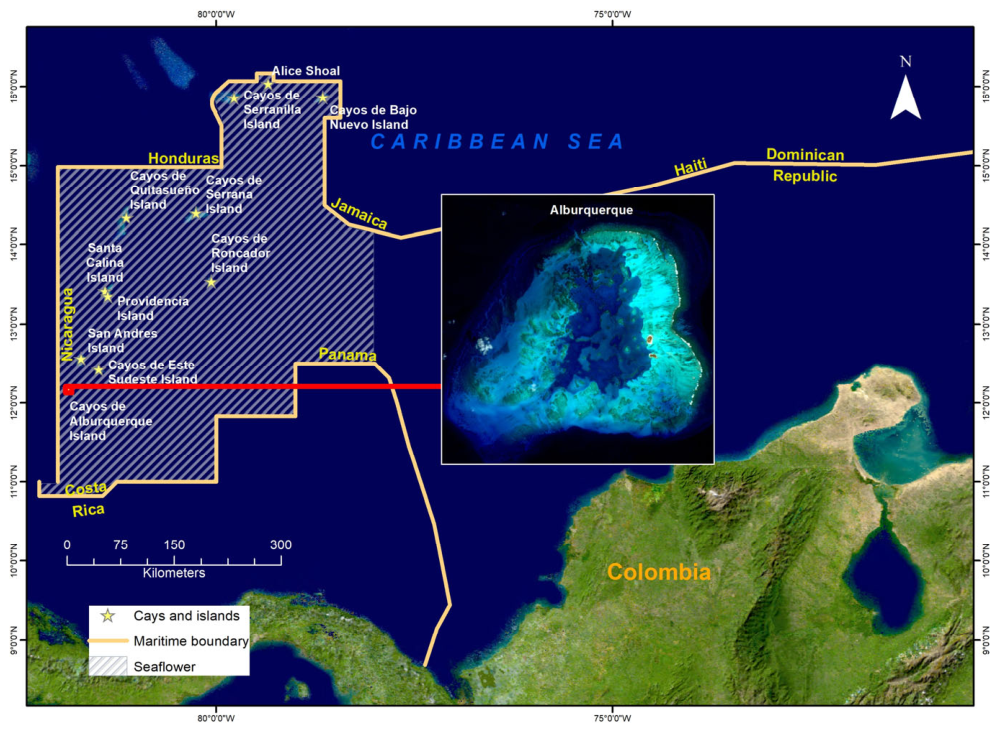
The study area corresponds to Cayo Alburquerque, located at the southern end of the archipelago, in a hard-to-access oceanic coral reef setting with limited official bathymetric coverage (Figure 1). Alburquerque Bank lies between 12 degrees 08 min and 12 degrees 12 min N and between 81 degrees 49 min and 81 degrees 54 min W, covers an area of 63.8 square kilometers, and is located approximately 35 km southwest of San Andres Island. Its morphology is essentially circular, with a fore reef terrace, and its east-to-west diameter exceeds 8 km. The atoll includes two cays, North Cay and South Cay, with a combined emergent area of approximately 0.1 square kilometers [39,42].
From a geomorphological perspective, the windward margin, comprising the northern, eastern, and southeastern quadrants, is characterized by a gently sloping terrace that abruptly transitions into a steep outer slope. The slope break occurs between 24 and 30 m of depth. Around this depth, a subhorizontal step is observed, predominantly covered by calcareous sediments, which encircles much of the atoll perimeter [43,44].

2.2. PlanetScope and ICESat 2 Data Area

PlanetScope Preprocessing and Quality Screening

PlanetScope reflectance was screened using UDM2/UDM2.1 (Usable Data Mask) to remove pixels affected by clouds, cloud shadows, haze, and other unusable conditions [45]. A land–water mask was derived from NIR and Normalized Difference Water Index (NDWI) thresholds to restrict analysis to optically shallow water pixels. Sun-glint was corrected using an NIR-to-visible linear regression following the widely used Hedley approach, applied bandwise to the visible channels before SDB model calibration [21]. All subsequent modeling used the corrected surface reflectance for valid water pixels only. An eight-band PlanetScope scene with 3 m spatial resolution was used, acquired on 31 December 2025, with cloud cover less than or equal to 1 percent and processed to Surface Reflectance, Level 3B. PlanetScope is a high-revisit global Earth observation constellation based on a fleet of CubeSat-type platforms. The product specifications and processing chain were used as the primary technical reference. In addition, available information for SuperDove sensors and spectral performance reports targeting aquatic applications was considered. Before modeling, the Usable Data Mask UDM2 and UDM2.1 were applied to exclude pixels affected by clouds, shadows, and haze, following the publicly available technical documentation [45]. UDM2 and UDM2.1 are Planet quality layers that flag unusable pixels (e.g., clouds, cloud shadows, haze) and were used to restrict the analysis to valid water pixels.
ICESat-2 carries the Advanced Topographic Laser Altimeter System (ATLAS), a photon-counting lidar operating at 532 nm. ATLAS emits six beams arranged in three beam pairs (GT1, GT2, GT3). Each pair comprises one strong and one weak beam separated laterally by approximately 90 m, while the separation between adjacent beam pairs is about 3.3 km. The strong and weak beams differ in pulse energy and therefore in photon return density, but they share the same nominal along-track shot spacing [20,35].
The ATL03 product provides, for each detected photon event, geodetic position (latitude, longitude) and ellipsoidal height referenced to the WGS 84 system, together with geolocation metadata organized into segments of approximately 20 m along track. These segments include photon count information and auxiliary variables associated with geophysical corrections, enabling accurate reconstruction of beam trajectories. For bathymetric applications in optically clear waters, the green channel is preferred due to its greater penetration into the water column. This capability, combined with the high along-orbit sampling, supports the potential of ATLAS to detect shallow seafloor returns and to provide independent vertical control to complement satellite-derived bathymetry from imagery (SDB) [20]. The nominal along-track separation between consecutive ATLAS laser shots is approximately 0.7 m; however, the number of detected photons and the effective sampling density vary primarily with beam energy (strong vs. weak) and observing conditions, rather than with the shot spacing itself. At the 3 m PlanetScope pixel size, multiple ATL03 photon events can fall within a single pixel footprint, so more than one depth observation may be available per pixel after co-location and quality filtering.
Vertical reference, geoid, and tide handling: ATL03 photon elevations are provided in an ellipsoidal WGS 84 reference frame. In our workflow, bathymetric depth is defined as the difference between the locally estimated instantaneous sea surface and the refracted seafloor photon elevation (Section 2.3). Because both terms are derived within the same reference frame and within the same along-track window, geoid offsets and ocean-tide signals largely cancel in the depth difference. Accordingly, we did not apply an external geoid or tidal correction; remaining vertical uncertainty is instead dominated by photon classification, sea state, and refraction/geo-location effects, which we discuss explicitly in Section 4.

2.3. Bathymetric Photon Extraction

To process ICESat-2 data, we developed a script in ArcGIS Pro and integrated it into a toolbox titled Multispectral ICESat Bathymetry and SDB. The photon classification and selection strategy was informed by previously documented open approaches, particularly the C-SHELPh tool (Classification of Sub-aquatic Height Extracted Photons), which identifies dense clusters associated with the sea surface and seafloor on a fine grid, with default values on the order of 0.5 m in the vertical axis and 10 m along track, incorporates refraction correction, and exports only photons with consistent signal for subsequent modeling or regression [46].
The ArcGIS Pro toolbox supports: (1) importing ATL03 photons into a GIS-compatible format; (2) classifying returns attributable to the seafloor using density height profiles (pseudo-waveforms); (3) applying air–water refraction correction; and (4) documenting QA/QC diagnostics and processing parameters throughout the workflow. Although the workflow was informed by open approaches such as C-SHELPh and OpenOceans, we implemented an ArcGIS Pro integrated pipeline that ingests ATL03 photon events into GIS ready feature classes, detects the local sea surface and candidate seafloor photons using density height pseudo waveforms with robust surface estimation, separates bottom returns from background noise using vertical continuity and along track coherence criteria, and applies per photon air water refraction correction based on the locally estimated sea surface. The tool also records QA/QC diagnostics and processing parameters and exports standardized CSV and TXT reports to support traceability and reproducibility.
In this study, ATL03 photons intersecting Cayo Alburquerque were filtered in space and time (2019–2025) and processed through three stages. First, density-based clustering in height space was applied within moving along-track windows to identify the local sea-surface photon mode and a candidate subsurface (seafloor) cluster. Sea-surface elevation was estimated in 10–30 m windows using a robust estimator (median or M-estimator) applied to the surface cluster. Second, a vertical continuity and coherence filter separated bottom returns from background noise. Third, air–water refraction correction was applied at the photon level via ray tracing referenced to the locally estimated sea surface, adjusting both elevation and horizontal displacement. Photon depth was defined as the difference between the estimated instantaneous sea surface and the subsurface return elevation after refraction correction.
Surface and bottom photon detection incorporated adaptive histograms and signal-to-noise thresholds derived from ATL03 attributes, enabling the identification of photon groups with valid signals and the assignment of event-scale confidence levels [35]. Refraction correction was then applied at the photon level via ray tracing, using the locally estimated sea surface (windowed median) and the refractive index of water, following methodologies previously validated for ICESat-2 in reef environments [45]. In addition, recent evidence on the utility of green-to-blue and blue-to-green band-ratio type predictors as complementary variables, and their use jointly with ICESat-2 for regional training and validation, was considered [36,46].
Using this procedure, 17 ATL03 ground tracks overlapping the cayo were compiled and, after quality control including masking of foam or breaking wave zones and removal of photons with low signal probability, 5171 point depth observations were obtained. Of these, 5021 were retained as valid in water observations for model calibration with the PlanetScope scene. Within the study area, 17,458 geolocated photon events were imported from the 17 ATL03 tracks. The workflow retained 5171 candidate seafloor depth observations after classification and quality control (29.6% of imported photon events), and 5021 points remained after intersecting with the PlanetScope water mask and removing non-useable reflectance samples (28.8%). The resulting bathymetric photons serve as a point reference for training and validation of the SDB models and support the methodological comparison among the spectral approaches evaluated in this work.

2.4. Bathymetric Models

Satellite-derived bathymetry (SDB) from multispectral sensors in shallow waters is grounded in the exponential attenuation of radiation within the water column and its additional modulation by bottom reflectance. Within this framework, empirical approaches estimate depth Z using linear or nonlinear relationships between Z and combinations of logarithmic transforms of visible-band reflectance, typically in the blue and green spectral regions. These formulations aim to reduce sensitivity to variations in benthic albedo and to changes in the optical state of the water. Such approaches coexist with radiative-transfer-based methods and, more recently, machine-learning schemes. Together, they constitute the methodological repertoire widely synthesized in recent reviews of coastal SDB [36].
In this study, depth Z was estimated using four classical empirical formulations, selected for their broad adoption in reefs, lagoons, and shallow platforms, as well as for their compatibility with 8-band PlanetScope imagery in combination with ICESat-2 (ATL03)-derived bathymetric control points. Recent evidence indicates that ICESat-2 bathymetric photons, when properly classified and corrected for refraction, provide a reliable reference source and do not exhibit systematic habitat-related biases, which supports their use for calibration and validation of empirical SDB in reef environments [36]. After classification and QA/QC, 5171 refraction-corrected ICESat-2 seafloor depth observations were obtained; after intersecting with the PlanetScope water mask and excluding unusable reflectance samples, 5021 points were retained for model calibration and validation. The candidate co-localized dataset (n = 5171) intersected N = 5077 unique PlanetScope 3 m pixels. Because ICESat-2 provides sub-meter along-track sampling, multiple points may fall within the same PlanetScope pixel. The number of points per pixel ranged from 1 to 2 (median = 1.00, p95 = 1.00). Point-to-pixel center offsets were bounded by the 3 m pixel geometry (maximum ~2.12 m) and showed a median = 1.21 m (p95 = 1.80 m). We discuss the implications of repeated sampling per pixel and mitigate spatial dependence through non-replacement, depth-stratified train–validation splits (70/30, 80/20, and 90/10) complemented with track-level jackknife resampling.
Note on machine-learning SDB. We acknowledge that machine-learning and deep-learning approaches (e.g., random forests and CNN-based regressors) have recently shown strong performance in optically complex shallow waters. In this study, we prioritize empirically grounded and interpretable formulations that can be calibrated with sparse, photon-based control and that integrate cleanly into a transparent ArcGIS Pro workflow. Extending the comparison to machine learning and deep learning (ML/DL) models, while feasible with the same input data, would require additional hyperparameter tuning, cross-validation design, and reporting that are beyond the scope of this revision; we therefore identify ML/DL benchmarking as a priority for future work.

2.4.1. Lyzenga (1985) [46] Linear Multiband Regression

The Lyzenga (1985) [46] algorithm models water depth Z from the spectral attenuation of radiance within the water column, conceptually grounded in the Beer-Lambert law. In its empirical formulation, Z is estimated as a linear combination of the natural logarithms of reflectance in visible bands, typically blue and green, to approximate the relationship between depth and the attenuated spectral signal. The central premise is that, under approximately homogeneous optical conditions, a linear relationship exists between depth and the logarithmic response of these bands:
Z = a + b 1 ln R B + b 2 ln R G .
where R B and R G denote reflectance in the blue and green bands, respectively, and a , b 1 , and b 2 are fitted parameters.
The multiband formulation helps reduce the influence of benthic albedo, insofar as part of the variability associated with bottom reflectance is absorbed by the multivariate term, while assuming that the water column remains optically homogeneous within the analyzed area. In this study, the coefficients a b 1 b 2 were estimated using ordinary least squares (OLS) under training partitions of 70%, 80%, and 90% of the refraction corrected bathymetric photons. The calibrated model was then applied at the pixel level, and its performance was evaluated in terms of goodness-of-fit and coefficient stability, consistent with its widespread use as an empirical baseline in SDB studies [36,46].

2.4.2. Lyzenga (2006) [47]: Nonlinear Polynomial Model

To represent nonlinearities associated with spectral attenuation and complex interactions at the water substrate interface, we implemented a polynomial extension of the Lyzenga approach [47]. This formulation extends the classic linear scheme by incorporating quadratic terms and a cross-term between bands, thereby increasing model flexibility in clear waters with mixed or heterogeneous benthic substrates. The quadratic model was defined using log-transformed predictors as:
Z = a + b 1 ln R B x y 2 + b 2 ln R G + c 1 l n 2 R B + c 2 l n 2 R G + c 3 ln R B ln R G .
where R B and R G represent reflectance in the blue and green bands, respectively, and a b 1 b 2 c 1 c 2 c 3 were estimated using ordinary least squares (OLS).
This configuration enables the model to capture curvature and spectral-coupling effects that cannot be represented by a strictly linear formulation, potentially reducing biases associated with moderate spatial variability in water optics and benthic albedo. However, the additional degrees of freedom may increase estimator variance and the risk of overfitting, particularly under high spectral collinearity or when the reflectance dynamic range is limited. To control these effects, we conducted nested comparisons against the linear model, inspected the signs and magnitudes of c 1 , c 2 , and c 3 , and evaluated the stability of performance metrics under changes in the training proportion. This variant was adopted only when gains in R 2 and reductions in RMSE were consistent across partitions and did not compromise generalization. This formulation and its use in SDB have been widely documented and are frequently cited alongside the Stumpf algorithm [46,48].

2.4.3. Stumpf et al. (2003) [17]: Normalized Log Ratio Index

The algorithm of Stumpf et al. (2003) [17] estimates depth using a log-ratio index designed to reduce sensitivity to variations in bottom albedo. The method relates depth Z to the logarithm of the ratio between blue and green water-leaving reflectances, scaled by a constant n and calibrated with two coefficients (m1, m0). We verified the transcription against the original formulation; the choice of logarithm base (ln versus log10) rescales m1 and does not affect model structure, because coefficients are estimated from the calibration data.
Z = a + b l n n R B R G
where R B and R G are the reflectances in the blue and green bands, respectively; a   and b are fitted parameters; and n is a scaling factor.
The ratio R B / R G tends to be relatively invariant to proportional changes in benthic albedo, provided that the ratio of attenuation coefficients remains approximately stable at the local scale. Operationally, the method offers advantages due to its parsimony, its relative robustness to substrate variability, and its direct raster implementation. However, because it relies on a single predictor, it is less flexible in representing curvature and complex spatial optical gradients, leading to higher RMSE than multiband formulations that include nonlinear terms.
In this study, the factor n was fixed to keep the logarithm argument within a numerically stable range, and the spectral pair was restricted to the PlanetScope blue and green bands, as these maximize bathymetric sensitivity in clear waters and reduce the influence of noise sources present in other spectral regions. Although the method is widely used, it is acknowledged to tend to overestimate depths over dark bottoms and underestimate depths over bright bottoms, a pattern reported in recent applications validated with LiDAR or sonar [17,37,49].

2.4.4. Bierwirth (1993) [49]: Ratio Model with Relative Attenuation Parameter

The Bierwirth et al. (1993) [49] approach introduces a depth index that is approximately bottom-invariant, formulated from log-transformed reflectance and a relative attenuation parameter between bands. Operationally, depth Z is fitted using a linear combination of the natural logarithms of reflectance in the blue and green bands:
Z = a + b 1 ln R B + b 2 ln R G
where R B and R G denote reflectance in the blue and green bands, respectively, and a , b 1 , and b 2 are estimated by ordinary least squares. From the fitted coefficients, an effective relative attenuation parameter is defined as:
k = b 2 b 1
In the empirical interpretation of the model, k acts as a spectral correction term that compensates for the different penetrations of blue and green light within the water column, thereby summarizing the site-specific relationship between band extinction coefficients. This formulation remains widely used and is frequently cited in reviews of empirical SDB methods, with reported applications in reef environments [36,50].

2.5. Calibration and Validation

We built a reference table by sampling PlanetScope reflectance at each refraction-corrected ATL03 seafloor point. After photon QA/QC, 5171 candidate seafloor observations intersected the PlanetScope scene, applying the water/quality masks and reflectance screening described in Section 2.2. yielded 5021 co-located samples for calibration and independent validation. To ensure fair comparison across models, the same filtered sample set and identical train/validation partitions were used for all algorithms. Splits were generated without replacement using a fixed random seed (Seed = 42) and stratified by depth bins ([−20, −10, −5, 0] m) to balance depth distributions across train/validation subsets.
We evaluated three calibration fractions (70%, 80%, and 90%) and held the remaining samples out for independent validation (30%, 20%, and 10%). Model parameters were estimated by ordinary least squares (with multivariate quadratic terms, as in Lyzenga 2006). Predictive performance was assessed on held-out data using root mean square error (RMSE), mean absolute error (MAE), bias, and the coefficient of determination R2 computed as R2 = 1 − SSE/SST. Because ICESat-2 provides dense along-track sampling, multiple photons may fall within the same 3 m PlanetScope pixel. We therefore report pixel-level sampling diagnostics (unique pixels, points per pixel, and point-to-pixel-center offsets) and mitigate spatial dependence by using depth-stratified splitting and reporting split-specific depth distributions (Section 3.1). Uncertainty budget framework: For reporting and interpretation, we treat overall SDB uncertainty as a combination of independent contributions from (1) ICESat-2 photon classification and geolocation, (2) residual air-to-water refraction effects after correction, (3) PlanetScope radiometric noise and residual atmospheric or sun-glint artifacts after preprocessing, and (4) model-parameter uncertainty. Conceptually, these contributions can be expressed as σ_total2 ≈ σ_ICESat22 + σ_refraction2 + σ_radiometry2 + σ_model2. In this study, σ_model is captured operationally by independent validation residuals, and we report depth-stratified errors for the optimal model.

2.6. Implementation and Toolbox

The methodological workflow was implemented in ArcGIS Pro using Python 3.10 and ArcPy through a custom toolbox designed with a modular, traceable, and reproducibility-oriented architecture. Two widely used open-source development frameworks informed the design. The first is OpenOceans, which focuses on assisted photon curation and classification, including separation of surface and seafloor returns, with support for expert auditing in complex segments [49]. The second is C-SHELPh, which emphasizes automated extraction of bathymetric photons and their integration with SDB modeling and regression [50,51].
The toolbox was organized into two primary tools. The first, ICESat-2 Ingestion, reads ATL03 files in HDF5 format, performs spatiotemporal subsetting, applies flags and variables from the ATL03 data dictionary, organizes data by beam, and manages spatial partitioning for processing. It then classifies photons using a dual scheme that combines OpenOceans-style assisted curation with a C-SHELPh-type automated procedure based on dense binning and mode separation to identify surface and bottom clusters. Next, it applies air water refraction correction and vertical harmonization, with an optional geoid adjustment, before exporting a bathymetric feature class accompanied by quality metadata. Toolbox availability: The ArcGIS Pro toolbox package and a concise user guide, including tool parameters and an example workflow, are provided as Supplementary Materials. Licensing constraints restrict the distribution of PlanetScope imagery.
The second tool, SDB Models, applies the PlanetScope preprocessing described in Section 2.2. (UDM screening, water masking, and sun-glint correction), links bathymetric points with raster reflectance, and then fits and evaluates the selected SDB model(s) under user-specified train/validation splits. It outputs the calibrated model coefficients, predicted SDB rasters, and per-split performance reports.
Across the workflow, the system records execution parameters, applied masks, random seeds, dependency versions, and reproducible logs to ensure auditability and repeatability. It also incorporates PlanetScope product technical documentation and SuperDove sensor information as a basis for decisions on band selection and mask usage. It maintains conceptual compatibility with the community evolution of ATL03-related products and algorithms. This approach facilitates the adoption of open best practices and supports transferring the workflow to other insular settings with limited bathymetric data availability.

3. Results

3.1. Vertical Control Points

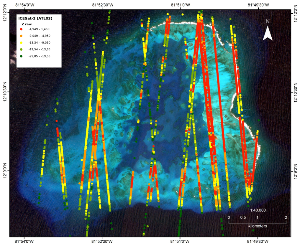
The vertical control dataset derived from ICESat-2 comprised 17 ATL03 ground tracks and 5171 point observations. After quality control and intersection with the water mask, 5021 valid points were retained (Figure 2). Depths were concentrated within the target shallow-water interval, approximately 0 to 20 m.
For model evaluation, three non-replacement, depth-stratified train validation splits were implemented: 70 30, with training n = 3515 and validation n = 1506; 80 20, with training n = 4017 and validation n = 1004; and 90 10, with training n = 4519 and validation n = 502. The use of ICESat-2 points as a vertical reference is consistent with previous studies reporting seafloor returns after refraction correction and sub-meter accuracies in clear waters, as well as their utility for training multispectral SDB models at regional scales [18,30].

3.2. Overall Performance by Algorithm

In the independent validation (Table 1), the comparative analysis showed a consistent pattern across partitions (70/30, 80/20, and 90/10). Overall, Lyzenga et al. (2006) [47] provided the best combination of goodness-of-fit and error magnitude, followed closely by Bierwirth et al. (1993) [49]. Lyzenga (1985) [46] exhibited intermediate performance, whereas Stumpf et al. (2003) [17] yielded unsatisfactory results under the conditions of this case study.
Lyzenga et al. (2006) [47] achieved the strongest indicators across the three partitions, with low and slightly negative bias. The 80/20 partition produced the minimum RMSE, and differences among partitions were minor, suggesting that model performance is stable under reasonable changes in the training proportion. This consistency across 70/30, 80/20, and 90/10, together with the depth-stratified splitting strategy, serves as a practical sensitivity check of Lyzenga et al. (2006) [47] to training sample size and depth distribution under the available data. Bierwirth et al. (1993) [49] delivered comparable performance and a positive bias, consistent with a slight overestimation. For this formulation, moderate degradation was observed under the 90/10 partition, consistent with the expected increase in uncertainty as the validation sample size decreases.
By contrast, Lyzenga (1985) [46] showed lower performance than the two previous formulations and a negative bias. This result suggests that the simpler linear parameterization captures spatial optical variability less effectively than the extended formulation of Lyzenga et al. (2006) [47]. Finally, Stumpf et al. (2003) [17] produced strongly negative R2 values, high RMSE, and an increasing positive bias. In practical terms, these indicators show that the log-ratio formulation does not reproduce the reflectance-depth relationship observed during validation under the study conditions and the applied preprocessing; therefore, its adoption as an operational model is not justified for this case. Strongly negative R2 values are mathematically possible because R2 = 1 − SSE/SST. When prediction errors are much larger than the variance of the reference depths (SSE much greater than SST), R2 becomes negative and can reach large magnitudes. In our case, the Stumpf log-ratio formulation produced large residuals across the validation range, which explains both the high RMSE and the strongly negative R2 values.
Overall, the observed patterns are consistent with reports in the literature indicating that, in optically shallow environments, multiband attenuation-based models tend to outperform log ratio indices, and that Lyzenga-type formulations remain competitive baselines when calibrated with independent control data [18,20].
To complement the global metrics in Table 1, Table 2 reports depth-stratified validation errors for the best-performing model Lyzenga et al. (2006) [47] under the 80/20 partition.
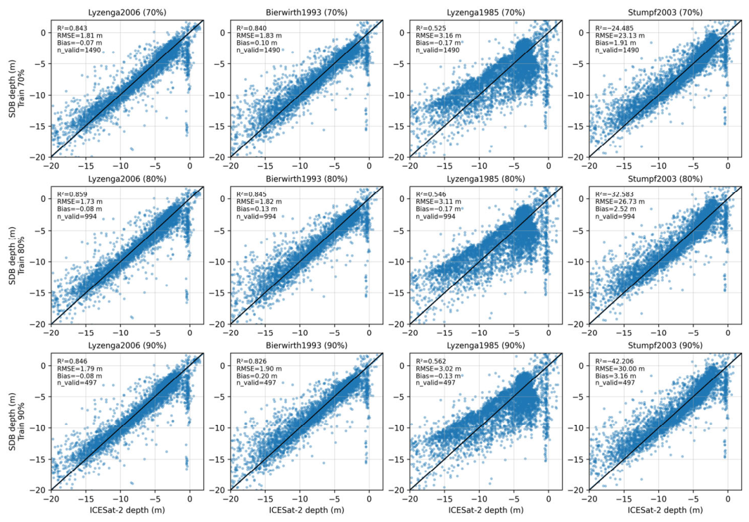
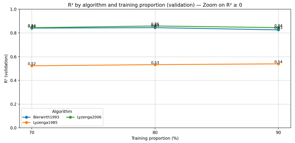
Figure 3 summarizes comparative validation performance and confirms the relative advantage of the multiband approaches, particularly Lyzenga et al. (2006) [47] and, at a secondary level, Bierwirth et al. (1993) [49], both of which show high R2 values and minimal variation across training proportions. Quantitatively, Lyzenga et al. (2006) [47] maintained R2 = 0.843 to 0.859 (RMSE = 1.734 to 1.813 m; bias = −0.070 to −0.081 m), whereas Bierwirth 1993 yielded R2 = 0.826 to 0.845 (RMSE = 1.818 to 1.904 m; bias = 0.100 to 0.205 m). In contrast, Lyzenga (1985) [46] exhibited substantially lower goodness of fit (approximately R2 = 0.52 to 0.56 in Figure 3), suggesting that the simpler linear formulation has limited capacity to represent the spatial optical variability of the site under the applied preprocessing. Complementarily, Figure 3 provides scatter plots of ICESat-2 reference depths versus SDB estimates for all evaluated models and partitions, enabling visual inspection of bias patterns and outlier structure that summary metrics alone cannot fully convey.
By comparison, Stumpf et al. (2003) [17] reported negative R2 values (−24.5 to −42.2) and markedly larger errors (RMSE = 23 to 30 m; bias = 1.9 to 3.2 m). Because Figure 4 zooms in on R2 ≥ 0, this behavior is not shown in the plot; however, the results indicate that the log-ratio scheme fails to reproduce the reflectance-depth relationship observed during validation for the evaluated conditions. This pattern is consistent with prior reports emphasizing the sensitivity of log-ratio indices to unmodeled curvature and optical gradients associated with bottom-type mixtures, spatial variability in water clarity, and habitat heterogeneity, which can degrade model fit when these nonlinearities are not explicitly represented [30].
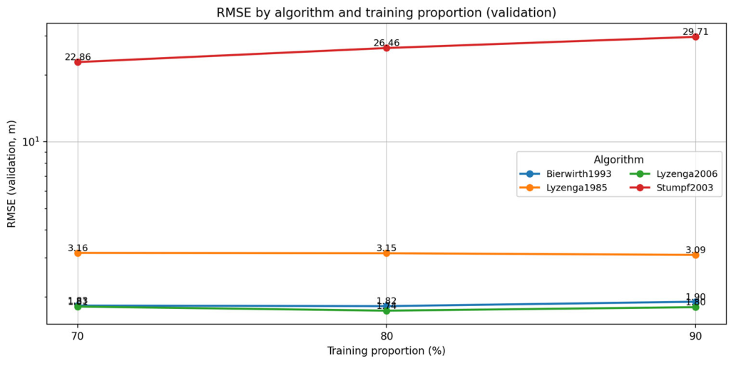
Complementarily, Figure 5 confirms the precision ranking observed in the independent validation. Lyzenga et al. (2006) [47] consistently yields the lowest errors, with RMSE values of 1.77 to 1.83 m, followed by Bierwirth et al. (1993) [49], with RMSE values of 1.82 to 1.90 m. In contrast, Lyzenga (1985) [46] reports markedly lower performance, with RMSE values of 3.09–3.16 m. Stumpf et al. (2003) [17] reports errors that are roughly an order of magnitude larger (RMSE = 22.86–29.71 m); therefore, the visualization was designed to preserve discrimination within the practical range of the best-performing models and to avoid loss of detail due to the full dynamic range.
The relatively low and stable global biases in the leading models are consistent with the expected effect of systematically removing sun glint using the NIR visible regression proposed by Hedley et al. (2005) [21], which reduces dispersion induced by specular reflectance and improves calibration robustness. Overall, the magnitude of the errors and the resulting ranking are consistent with international syntheses, which commonly report that multiband attenuation-based models outperform the log-ratio scheme in shallow waters and achieve comparable performance across multiband formulations in coastal settings [30]. Likewise, studies integrating ICESat-2 with multispectral imagery indicate that, when calibration is supported by properly processed seafloor photons, including explicit refraction correction, Lyzenga-type formulations tend to produce the lowest RMSE relative to alternative empirical and machine learning approaches in clear waters, while also enabling scalable operational workflows [18,49].
Global biases were low for the three formulations that produced physically consistent fits in validation (Lyzenga (1985) [46], Lyzenga et al. (2006) [47], and Bierwirth et al. (1993) [49]), with |Bias| ≤ 0.205 m across partitions, and values close to zero for Lyzenga (2006) (−0.070 to −0.081 m). Lyzenga (1985) [46] showed a slight negative bias (−0.172 to −0.130 m), whereas Bierwirth et al. (1993) [49] exhibited a slight positive bias (0.100 to 0.205 m), consistent with a slight overestimation. In contrast, Stumpf et al. (2003) [17] yielded substantially larger positive biases (1.906 to 3.155 m), in agreement with its strongly negative R2 and the order-of-magnitude increase in RMSE. This behavior is consistent with the known sensitivity of spectral ratio formulations to unmodeled optical gradients and curvature in the reflectance-depth relationship when background conditions vary spatially. The literature also indicates that sun glint removal via NIR-visible regression reduces variance induced by specular brightness and improves calibration stability, particularly under moderate wind conditions. Because this preprocessing step was applied systematically, the low biases observed for the best-performing models are consistent with expectations [21].
The error magnitudes and relative rankings across algorithms are consistent with international syntheses. In Irish coastal settings, multiband empirical formulations have been reported to outperform log-ratio approaches in shallow waters, with R2 values ranging from 0.83 to 0.88, comparable to the performance obtained here for Lyzenga et al. (2006) [47] despite differences in environment and sensor characteristics [30]. Similarly, studies integrating ICESat-2 with multispectral imagery have shown that Lyzenga-type formulations, when calibrated using refraction-corrected seafloor photons, tend to achieve the lowest RMSE relative to other empirical and machine learning alternatives in clear waters, while supporting scalable operational workflows at regional to national scales [18,49].
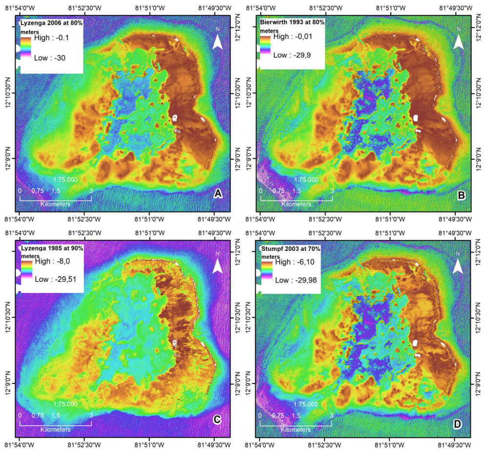
Finally, Figure 6 links the quantitative assessment to the cartographic product by displaying the resulting bathymetric surfaces and their spatial coherence at the reef-unit scale. This visualization enables verification of geomorphological plausibility, including spatial continuity, the absence of localized artifacts, and visual correspondence with the reef-lagoon structure. In this way, the map-based evidence complements the statistical evaluation and strengthens the case for the selected workflow in bathymetric mapping of remote insular environments [18,49].

4. Discussion

PlanetScope (3 m surface reflectance, 8 bands, high revisit) enables reef-scale shallow-water bathymetry and operational updates in remote settings. We evaluated a PlanetScope-based SDB workflow calibrated and independently validated using ICESat-2 ATL03 photon-derived seafloor control, and compared four widely used empirical formulations across multiple training splits. A stable performance hierarchy emerged in which multiband approaches, particularly Lyzenga et al. (2006) [47] and Bierwirth et al. (1993) [49], consistently outperformed the Stumpf et al. (2003) [17] log-ratio model, while the simpler Lyzenga (1985) [46] linear formulation showed intermediate skill. This pattern indicates that PlanetScope visible bands preserve a usable bathymetric signal when strict masking and radiometric control are applied, and that higher-capacity multiband parameterizations are advantageous in high-resolution reef imagery affected by spatially variable optics and heterogeneous substrates [18,30].
Independent validation RMSEs of approximately 1.7–1.9 m are suitable for coastal geomorphology, habitat characterization, and management-oriented mapping, but remain insufficient for high-precision hydrographic applications. Accordingly, outputs should be interpreted within a clear domain of applicability and accompanied by uncertainty reporting that identifies depth ranges and settings where performance degrades (Table 2), together with diagnostic fit patterns (Figure 3). Although we do not introduce a separate geomorphic zoning layer in this revision, the depth strata in Table 2 provide a first-order proxy for reef geomorphic settings, for example, very shallow reef-flat and near-crest environments versus deeper fore-reef and lagoonal areas, which improves spatial interpretability of model errors with the available photon-based control. The modest and stable biases observed in the leading models are consistent with systematic NIR-to-visible regression deglinting and conservative masking of surf and foam, as well as residual specular contamination, which are key steps for isolating the bathymetric signal and reducing exogenous variance under wave- and wind-affected conditions [21].
ICESat-2 ATL03 provides repeatable, photon-traceable vertical control, helping address hydrographic data gaps on remote oceanic islands. This point-based reference supports calibration and uncertainty constraints for continuous, pixelwise optical bathymetry derived from passive sensors. Its utility depends on obtaining a coherent seafloor photon cluster and can be reduced by turbidity, surface roughness, foam, and elevated background noise, particularly in high-energy sectors where dispersion of surface returns complicates surface-to-seafloor separation. ATLAS is a photon-counting lidar, and bathymetric retrieval relies on detecting sparse bottom photons and applying air-to-water refraction correction. As an order-of-magnitude uncertainty statement, published clear-water comparisons against acoustic surveys commonly indicate decimeter-to-meter vertical errors for ICESat-2-derived bathymetry after refraction correction, with uncertainty increasing under higher turbidity and rougher sea states [19,30,44,45,46]. In our workflow, the dominant contributions are expected to arise from photon classification and residual refraction effects in challenging conditions, while PlanetScope radiometric noise and residual preprocessing artifacts (including sun-glint) contribute additional variance to the optical inversion. Spatial support also differs: ICESat-2 samples are point-based within an approximately 11–13 m footprint with sub-meter along-track sampling, whereas PlanetScope estimates depth over 3 m pixel areas. Therefore, ICESat-2 offers valuable independent vertical control for benchmarking and uncertainty constraints, but it does not replace hydrographic-grade echo sounding when charting standards are required.
Residuals in this study are larger than those reported in some clear-water SDB work (e.g., [52]), likely reflecting combined effects of heterogeneous benthic cover and adjacency at reef edges, residual sun glint and atmospheric artifacts despite correction, sensor spectral-response differences, and depths approaching the optical limit. To reduce sensitivity to depth-range imbalance, we used depth-stratified calibration and validation splits and explicitly reported depth distributions. Future work may further stabilize performance by adopting sampling designs that balance depth and optical classes and, where feasible, incorporate bottom-type stratification following PTID-like guidance [53,54].
Because the continuous SDB raster is produced by applying the calibrated spectral model pixelwise rather than interpolating ICESat-2 depths, predictive reliability can decrease where ATL03 tracks poorly represent local conditions. Differences in calibrated depth range, track coverage across geomorphic settings, and spatial variability in water optics and benthic reflectance can increase uncertainty and lead to localized artifacts, particularly near sharp habitat transitions and in high-energy shallow zones. Areas with sparse or absent ICESat-2 control should therefore be interpreted cautiously.
Uncertainty in a fully spaceborne SDB workflow reflects multiple coupled sources, including ICESat-2 photon classification and geolocation uncertainty, residual refraction error after correction, PlanetScope radiometric noise and residual atmospheric or sun-glint effects, and model-parameter uncertainty from finite and depth-heterogeneous training samples. Conceptually, these terms form a combined uncertainty budget (for example, σ_total2 ≈ σ_ICESat22 + σ_refraction2 + σ_radiometry2 + σ_model2) whose relative importance varies with depth, bottom type, and optical conditions. Given a photon-based reference rather than dense echo-sounder gridding, we report uncertainty primarily through independent validation RMSE and bias across multiple train-to-validation partitions and through depth-stratified errors for the optimal model (Table 2), providing an operational envelope within the stated domain of applicability (0 to 20 m, clear-water conditions). Depth strata can also be interpreted as a first-order proxy for reef geomorphic settings in this atoll, with 0–5 m broadly corresponding to reef-flat and shallow-lagoon environments and deeper strata representing fore-reef and upper-slope contexts.
Transfer to other reef sites should follow a standardized, auditable protocol: select scenes with low turbidity and favorable sea state, apply UDM2 or UDM2.1 screening with conservative water masking, recalibrate coefficients per scene using locally co-located ICESat-2 control points, and report validation metrics and uncertainty with respect to depth and preprocessing limits. Within these constraints, the ArcGIS Pro toolbox supports the production of reproducible, research-grade reef-scale bathymetry products for regions with limited in situ hydrographic coverage. Extending comparisons to machine learning or deep learning approaches [55,56] remains a priority for future work, but only under the same requirements for independent validation, traceability, and systematic uncertainty reporting [18,30].
Finally, multiband formulations (Lyzenga et al. (2006) [47]; Bierwirth et al. (1993) [49]) outperformed the Stumpf et al. (2003) [17] log-ratio model under the evaluated reef conditions. The log-ratio compresses spectral information into a single index and is therefore more sensitive to residual glint, adjacency effects, and benthic heterogeneity that alter reflectance in wavelength-dependent ways. In the study area, variability in blue and green reflectance driven by benthic heterogeneity, subtle water-clarity gradients, and residual sun-glint can introduce curvature and band-dependent effects that violate the single-ratio assumption of Stumpf et al. (2003) [17]. This helps explain the bias structure and the outliers visible in Figure 3, as well as the strongly negative out-of-sample R2 obtained during independent validation. In contrast, multiband structures exploit additional spectral degrees of freedom, including cross-band coupling and, in the curvilinear extension, nonlinear terms, which better accommodate spatially varying bottom reflectance and subtle optical gradients that violate uniform attenuation assumptions. The strongly negative out-of-sample R2 for Stumpf et al. (2003) [17] is consistent with model misspecification under these conditions rather than a computational artifact, highlighting the importance of matching model structure to site-specific reef optics and preprocessing limits.

5. Conclusions

This study demonstrates the technical and operational feasibility of producing satellite-derived bathymetry (SDB) in remote coral reef environments using PlanetScope surface reflectance imagery. The core contribution is a reproducible PlanetScope-based workflow that leverages 3 m spatial resolution and an 8-band multispectral configuration to retrieve reef-scale bathymetric patterns, while using ICESat-2 (ATL03) photon-derived seafloor picks as independent, traceable vertical control for calibration and validation.
Across three training partitions (70/30, 80/20, and 90/10), the PlanetScope results show a stable performance hierarchy. Lyzenga et al. (2006) [47] was consistently the most robust formulation (R2 approximately 0.84 to 0.86; RMSE 1.73 to 1.81 m; low bias near zero), followed closely by Bierwirth et al. (1993) [49] (R2 0.83 to 0.85; RMSE 1.82 to 1.90 m; moderate positive bias). Lyzenga (1985) [46] was less accurate (RMSE near 3.0 m), and Stumpf et al. (2003) [17] were not suitable under the evaluated optical conditions due to strongly degraded validation performance.
A central methodological finding is that PlanetScope SDB performance depends critically on radiometric and geometric quality control. UDM2 or UDM2.1 masking, NIR-visible regression-based sun-glint correction, conservative exclusion of surf and foam, and per-photon air-water refraction correction for ICESat-2 seafloor picks are necessary steps to stabilize calibration and mitigate systematic errors in high-energy shallow settings. To ensure reproducibility and traceability, the workflow was implemented as a modular ArcGIS Pro toolbox that records QA/QC metrics and exports CSV and TXT reports, facilitating transfer to other reef settings and monitoring programs, while acknowledging the practical implications of PlanetScope data access and licensing.
Overall, the results support PlanetScope as a viable high-resolution input for SDB mapping and reef monitoring when calibrated within the depth range represented by photon control and interpreted within a clearly defined optical domain. Operational use should prioritize rigorous scene selection, explicit uncertainty reporting stratified by depth and habitat, and avoidance of extrapolation beyond validated conditions. Spatial confidence is expected to decrease where local optics or substrates depart from those sampled by the ICESat-2 tracks, particularly in areas far from control observations.

Supplementary Materials

The following supporting information can be downloaded at: https://www.mdpi.com/article/10.3390/geomatics6020039/s1, ICESat bathymetry and SDB_Toolbox.zip.

Funding

This work was funded in part by the AGESAT Research Group, Universidad del Valle. No specific external grant number was associated with this work.

Data Availability Statement

The PlanetScope imagery used in this study is subject to licensing restrictions and cannot be publicly shared. Derived datasets and processing outputs may be made available by the author upon reasonable request, subject to licensing and data-access restrictions. ICESat-2 ATL03 data are publicly available from NASA NSIDC.

Conflicts of Interest

The author declares no conflicts of interest.

References

  1. Almar, R.; Bergsma, E.W.J.; Thoumyre, G.; Baba, M.W.; Cesbron, G.; Daly, C.; Garlan, T.; Lifermann, A. Global Satellite-Based Coastal Bathymetry from Waves. Remote Sens. 2021, 13, 4628. [Google Scholar] [CrossRef]
  2. Ashphaq, M.; Srivastava, P.K.; Mitra, D. Review of near-shore satellite-derived bathymetry: Classification and account of five decades of coastal bathymetry research. J. Ocean Eng. Sci. 2021, 6, 340–359. [Google Scholar] [CrossRef]
  3. Ashphaq, M.; Srivastava, P.K.; Mitra, D. Preliminary examination of influence of Chlorophyll, Total Suspended Material, and Turbidity on Satellite Derived-Bathymetry estimation in coastal turbid water. Reg. Stud. Ma-Rine Sci. 2023, 62, 102920. [Google Scholar] [CrossRef]
  4. Chen, H.; Cheng, L.; Zhang, K. Bathymetry-guided multi-source remote sensing image domain adaptive coral reef benthic habitat classification. GIScience Remote Sens. 2025, 62, 2471193. [Google Scholar] [CrossRef]
  5. Fuentes, J.E.; Moya, F.D.; Montoya, O.D. Method for Estimating Solar Energy Potential Based on Photogrammetry from Unmanned Aerial Vehicles. Electronics 2020, 9, 2144. [Google Scholar] [CrossRef]
  6. Janowski, Ł.; Tęgowski, J.; Montereale-Gavazzi, G. Editorial: Seafloor mapping using underwater remote sensing approaches. Front. Earth Sci. 2023, 11, 1306202. [Google Scholar] [CrossRef]
  7. Liu, Y.; Zhao, J.; Deng, R.; Liang, Y.; Gao, Y.; Chen, Q.; Xiong, L.; Liu, Y.; Tang, Y.; Tang, D. A downscaled bathymetric mapping approach combining multitemporal Landsat-8 and high spatial resolution imagery: Demon-strations from clear to turbid waters. ISPRS J. Photogramm. Remote Sens. 2021, 180, 65–81. [Google Scholar] [CrossRef]
  8. Su, H.; Liu, H.; Wang, L.; Filippi, A.M.; Heyman, W.D.; Beck, R.A. Geographically Adaptive Inversion Model for Improving Bathymetric Retrieval from Satellite Multispectral Imagery. IEEE Trans. Geosci. Remote Sens. 2014, 52, 465–476. [Google Scholar] [CrossRef]
  9. Uzakara, H.; Demir, N.; Karakış, S. Satellite-based Bathymetry Supported by Extracted Coastlines. PFG—J. Photogramm. Remote Sens. Geoinf. Sci. 2024, 92, 317–334. [Google Scholar] [CrossRef]
  10. Wang, Y.; He, X.; Bai, Y.; Wang, D.; Zhu, Q.; Gong, F.; Yang, D.; Li, T. Satellite retrieval of benthic reflectance by combining lidar and passive high-resolution imagery: Case-I water. Remote Sens. Environ. 2022, 272, 112955. [Google Scholar] [CrossRef]
  11. Zhao, Y.; Yu, X.; Hu, B.; Chen, R. A Multi-Source Convolutional Neural Network for Lidar Bathymetry Data Classification. Mar. Geod. 2022, 45, 232–250. [Google Scholar] [CrossRef]
  12. Brando, V.E.; Anstee, J.M.; Wettle, M.; Dekker, A.G.; Phinn, S.R.; Roelfsema, C. A physics based retrieval and quality assessment of bathymetry from suboptimal hyperspectral data. Remote Sens. Environ. 2009, 113, 755–770. [Google Scholar] [CrossRef]
  13. Lee, Z.; Carder, K.L.; Mobley, C.D.; Steward, R.G.; Patch, J.S. Hyperspectral remote sensing for shallow waters. I. A semianalytical model. Appl. Opt. 1998, 37, 6329–6338. [Google Scholar] [CrossRef] [PubMed]
  14. Lee, Z.; Carder, K.L.; Mobley, C.D.; Steward, R.G.; Patch, J.S. Hyperspectral remote sensing for shallow waters. 2. Deriving bottom depths and water properties by optimization. Appl. Opt. 1999, 38, 3831–3843. [Google Scholar] [CrossRef] [PubMed]
  15. Mudiyanselage, S.S.J.D.; Abd-Elrahman, A.; Wilkinson, B.; Lecours, V. Satellite-derived bathymetry using machine learning and optimal Sentinel-2 imagery in South-West Florida coastal waters. GIScience Remote Sens. 2022, 59, 1143–1158. [Google Scholar] [CrossRef]
  16. Santos, R.; Quartau, R.; Lamas, L.; Cândido, R.; Pinto, J.P. Application of Neural Networks for Bathymetric Es-timation Using a Short Time-Series of Sentinel-2 Images: A Case Study on the Setúbal–Tróia Coastal Area. Remote Sens. Appl. Soc. Environ. 2025, 39, 101683. [Google Scholar] [CrossRef]
  17. Stumpf, R.P.; Holderied, K.; Sinclair, M. Determination of water depth with high-resolution satellite imagery over variable bottom types. Limnol. Oceanogr. 2003, 48, 547–556. [Google Scholar] [CrossRef]
  18. Thomas, N.; Pertiwi, A.P.; Traganos, D.; Lagomasino, D.; Poursanidis, D.; Moreno, S.; Fatoyinbo, L. Space-Borne Cloud-Native Satellite-Derived Bathymetry (SDB) Models Using ICESat-2 And Sentinel-2. Geophys. Res. Lett. 2021, 48, e2020GL092170. [Google Scholar] [CrossRef]
  19. Geyman, E.C.; Maloof, A.C. A Simple Method for Extracting Water Depth from Multispectral Satellite Imagery in Regions of Variable Bottom Type. Earth Space Sci. 2019, 6, 527–537. [Google Scholar] [CrossRef]
  20. Parrish, C.E.; Magruder, L.A.; Neuenschwander, A.L.; Forfinski-Sarkozi, N.; Alonzo, M.; Jasinski, M. Validation of ICESat-2 ATLAS Bathymetry and Analysis of ATLAS Bathymetric Mapping Performance. Remote Sens. 2019, 11, 1634. [Google Scholar] [CrossRef]
  21. Hedley, J.D.; Harborne, A.R.; Mumby, P.J. Technical note: Simple and robust removal of sun glint for mapping shallow-water benthos. Int. J. Remote Sens. 2005, 26, 2107–2112. [Google Scholar] [CrossRef]
  22. Chen, Q.; Wang, N.; Chen, Z. Simultaneous mapping of nearshore bathymetry and waves based on phys-ics-informed deep learning. Coast. Eng. 2023, 183, 104337. [Google Scholar] [CrossRef]
  23. Almar, R.; Bergsma, E.W.J.; Thoumyre, G.; Solange, L.-C.; Loyer, S.; Artigues, S.; Salles, G.; Garlan, T.; Lifermann, A. Satellite-derived bathymetry from correlation of Sentinel-2 spectral bands to derive wave kinematics: Qualification of Sentinel-2 S2Shores estimates with hydro-graphic standards. Coast. Eng. 2024, 189, 104458. [Google Scholar] [CrossRef]
  24. Duan, Z.; Chu, S.; Cheng, L.; Ji, C.; Li, M.; Shen, W. Satellite-derived bathymetry using Landsat-8 and Sentinel-2A images: Assessment of atmospheric correction algorithms and depth derivation models in shallow waters. Opt. Express 2022, 30, 3238–3261. [Google Scholar] [CrossRef]
  25. Nicolas, K.M.; Drumetz, L.; Lefèvre, S.; Tiede, D.; Bajjouk, T.; Burnel, J.-C. Deep Learning-Based Bathymetry Mapping from Multispectral Satellite Data Around Europa Island. In Proceedings of EUCOMARE 2022: International Conference European Spatial Data for Coastal and Marine Remote Sensing; Springer: Cham, Switzerland, 2022; pp. 97–111. [Google Scholar]
  26. Pacheco, A.; Horta, J.; Loureiro, C.; Ferreira, Ó. Retrieval of nearshore bathymetry from Landsat 8 images: A tool for coastal monitoring in shallow waters. Remote Sens. Environ. 2015, 159, 102–116. [Google Scholar] [CrossRef]
  27. Patel, A.; Katiyar, S.K.; Prasad, V. Bathymetric Mapping for Shallow Water Using Landsat 8 via Artificial Neural Network Technique. In Proceedings of Recent Trends in Civil Engineering; Springer: Singapore, 2021; pp. 717–733. [Google Scholar]
  28. Qian, S.; Chen, Y.; Wang, W.; Zhang, G.; Li, L.; Hao, Z.; Wang, Y. Physics-guided deep neural networks for bathymetric mapping using Sentinel-2 multi-spectral imagery. Front. Mar. Sci. 2025, 12, 1636124. [Google Scholar] [CrossRef]
  29. Xie, C.; Chen, P.; Zhang, S.; Huang, H. Nearshore Bathymetry from ICESat-2 LiDAR and Sentinel-2 Imagery Datasets Using Physics-Informed CNN. Remote Sens. 2024, 16, 511. [Google Scholar] [CrossRef]
  30. Casal, G.; Monteys, X.; Hedley, J.; Harris, P.; Cahalane, C.; McCarthy, T. Assessment of empirical algorithms for bathymetry extraction using Sentinel-2 data. Int. J. Remote Sens. 2019, 40, 2855–2879. [Google Scholar] [CrossRef]
  31. Albright, A.; Glennie, C. Nearshore Bathymetry from Fusion of Sentinel-2 and ICESat-2 Observations. IEEE Geosci. Remote Sens. Lett. 2021, 18, 900–904. [Google Scholar] [CrossRef]
  32. Babbel, B.J.; Parrish, C.E.; Magruder, L.A. ICESat-2 Elevation Retrievals in Support of Satellite-Derived Ba-thymetry for Global Science Applications. Geophys. Res. Lett. 2021, 48, e2020GL090629. [Google Scholar] [CrossRef] [PubMed]
  33. Xie, C.; Chen, P.; Zhang, Z.; Pan, D. Satellite-derived bathymetry combined with Sentinel-2 and ICESat-2 datasets using machine learning. Front. Earth Sci. 2023, 11, 1111817. [Google Scholar] [CrossRef]
  34. Xu, N.; Wang, L.; Zhang, H.S.; Tang, S.; Mo, F.; Ma, X. Machine Learning Based Estimation of Coastal Bathymetry from ICESat-2 and Sentinel-2 Data. IEEE J. Sel. Top. Appl. Earth Obs. Remote Sens. 2024, 17, 1748–1755. [Google Scholar] [CrossRef]
  35. Neumann, T.; Brenner, A.; Hancock, D.; Robins, J.; Saba, J.; Harbeck, K.; Gibbons, A.; Lee, J.; Luthcke, S.; Rebold, T. Ice, cloud, and land elevation satellite (ICESat-2) project algorithm the-oretical basis document (ATBD) for global geolocated photons ATL03, version 6. In Ice Data Center Distributed Active Archive Center Data Set; Snow, N.N., Ed.; NASA: New York, NY, USA, 2023. [Google Scholar]
  36. Gleason, A.C.R.; Smith, R.; Purkis, S.J.; Goodrich, K.; Dempsey, A.; Mantero, A. The Prospect of Global Coral Reef Bathymetry by Combining Ice, Cloud, and Land Elevation Satellite-2 Altimetry with Multispectral Satellite Imagery. Front. Mar. Sci. 2021, 8, 694783. [Google Scholar] [CrossRef]
  37. Caballero, I.; Stumpf, R.P. Towards Routine Mapping of Shallow Bathymetry in Environments with Variable Turbidity: Contribution of Sentinel-2A/B Satellites Mission. Remote Sens. 2020, 12, 451. [Google Scholar] [CrossRef]
  38. Thomas, N.; Lee, B.; Coutts, O.; Bunting, P.; Lagomasino, D. A purely spaceborne open source approach for regional bathymetry mapping. IEEE Trans. Geosci. Remote Sens. 2022, 60, 4708109. [Google Scholar] [CrossRef]
  39. Andrade Amaya, C.A. Caracterización Morfológica y Dinámica Litoral de los Cayos Habitados del Archipiélago de San Andrés y Providencia, en el Caribe Colombiano; Escuela Naval de Cadetes “Almirante Padilla”, Facultad de Oceanografía Física, Armada Nacional, Fuerzas Militares de Colombia: Cartagena de Indias D.T. y C., Colombia, 2010. [Google Scholar]
  40. Ariza, A.; Ramírez, H.M. Modelo Batimétrico derivado de imágenes Landsat ETM+ en zonas de arrecifes tropi-cales. Rev. Cart. 2019, 90, 43–58. [Google Scholar] [CrossRef]
  41. Aguilera-Díaz, M. Geografía económica del Archipiélago de San Andrés, Providencia y Santa Catalina; Banco de la República: Bogotá, Colombia, 2016. [Google Scholar]
  42. López, M.; Muñoz, A.P.; Valderrama, L.; Herrera, M.A. Corales y geckos del del atolón Alburquerque durante la Expedición Seaflower 2018-Proyecto Colombia BIO. In Proceedings of Pontificia Universidad Javeriana-Cali; Pontificia Universidad Javeriana: Cali, Colombia, 2018. [Google Scholar]
  43. Díaz, J.M.; Díaz-Pulido, G.; Garzón-Ferreira, J.; Geister, J.; Sánchez, J.A.; Zea, S. Atlas de los Arrecifes Coralinos del Caribe Colombiano; Litoflash: Rome, Italy, 1996; Volume 2, pp. 1–83. [Google Scholar]
  44. Garay, J.; Castillo, F.; Andrade, C.; Aguilera, J.; Niño, L.; de la Pava, M.; López, W.; Márquez, G. Estudio oceanográfico del área insular y oceánica del Caribe colombiano: Archipiélago de San Andrés y Providencia y cayos vecinos. Bol. Cient. CIOH 1988, 9, 3–73. [Google Scholar] [CrossRef]
  45. Planet. Planet Imagery Product Specification: PlanetScope & RapidEye; Planet Team: San Francisco, CA, USA, 2022. [Google Scholar]
  46. Lyzenga, D.R. Shallow-water bathymetry using combined lidar and passive multispectral scanner data. Int. J. Remote Sens. 1985, 6, 115–125. [Google Scholar] [CrossRef]
  47. Lyzenga, D.R.; Malinas, N.P.; Tanis, F.J. Multispectral bathymetry using a simple physically based algorithm. IEEE Trans. Geosci. Remote Sens. 2006, 44, 2251–2259. [Google Scholar] [CrossRef]
  48. Niroumand-Jadidi, M.; Bovolo, F.; Bruzzone, L. SMART-SDB: Sample-specific multiple band ratio technique for satellite-derived bathymetry. Remote Sens. Environ. 2020, 251, 112091. [Google Scholar] [CrossRef]
  49. Bierwirth, P.N.; Lee, T.J.; Burne, R.V. Shallow sea-floor reflectance and water depth derived by unmixing mul-tispectral imagery. Photogramm. Eng. Remote Sens. 1993, 59, 331–338. [Google Scholar]
  50. Markel, J.; Magruder, L.A. An Open Source Tool for ICESat-2 Bathymetric Data Labeling and Depth Correction. In Proceedings of AGU Fall Meeting Abstracts; American Geophysical Union: Chicago, IL, USA, 2022; p. C12B-0570. [Google Scholar]
  51. Parrish, C.E.; Magruder, L.; Herzfeld, U.; Thomas, N.; Markel, J.; Jasinski, M.; Imahori, G.; Herrmann, J.; Trantow, T.; Borsa, A.; et al. ICESat-2 Bathymetry: Advances in Methods and Science. In Proceedings of the OCEANS 2022, Hampton Roads, VA, USA, 17–20 October 2022; pp. 1–6. [Google Scholar]
  52. Li, X.; Wang, S.; Zhao, J.; Li, J.; Zhang, H.; Pan, H. Methods to Improve the Accuracy of Satellite-Derived Ba-thymetry: A Case Study of the Qilianyu Islands. Remote Sens. 2023, 15, 5406. [Google Scholar] [CrossRef]
  53. Legleiter, C.J.; Kinzel, P.J.; Nelson, J.M. Sampling strategies to improve passive optical remote sensing of river bathymetry. Remote Sens. 2018, 10, 935. [Google Scholar] [CrossRef]
  54. Legleiter, C.J.; Fosness, R.L. Defining the limits of spectrally based bathymetric mapping: An evaluation of factors affecting depth retrieval in clear waters. Remote Sens. 2019, 11, 665. [Google Scholar] [CrossRef]
  55. Hartmann, D.; Gravey, M.; Price, T.D.; Nijland, W.; de Jong, S.M. Surveying Nearshore Bathymetry Using Multispectral and Hyperspectral Satellite Imagery and Machine Learning. Remote Sens. 2025, 17, 291. [Google Scholar] [CrossRef]
  56. Ye, M.; Yang, C.; Zhang, X.; Li, S.; Peng, X.; Li, Y.; Chen, T. Shallow Water Bathymetry Inversion Based on Machine Learning Using ICESat-2 and Sentinel-2 Data. Remote Sens. 2024, 16, 4603. [Google Scholar] [CrossRef]
Figure 1. Location of the study area: Cayo Alburquerque within the Seaflower Biosphere Reserve (Colombian Caribbean), in the regional context of the Archipelago of San Andres, Providencia, and Santa Catalina. Basemap and imagery: Esri World Imagery/World Ocean Base (Esri and contributors; accessed March 2026). Administrative boundaries and coastlines: Natural Earth (v5.1.2).
Geomatics 06 00039 g001
Figure 2. Distribution of refraction-corrected ICESat-2 photon-based depth observations (N = 5021) retained for model calibration/validation after QA/QC and water masking. The depth colormap is monotonic from shallow (warm colors) to deep (cool colors) and was verified against shoreline context.
Geomatics 06 00039 g002
Figure 3. Scatter plots of ICESat-2-derived reference depths (x-axis) versus SDB-inverted depths (y-axis) for all evaluated models (Lyzenga et al. (2006) [47]; Bierwirth et al. (1993) [49]; Lyzenga (1985) [46]; Stumpf et al. (2003) [17]) across the three training partitions (70/30, 80/20, 90/10). The 1:1 line is shown for reference; annotations report validation metrics (R2, RMSE, bias) for each partition (Table 1).
Geomatics 06 00039 g003
Figure 4. Coefficient of determination (R2) by algorithm and training proportion (70, 80, and 90 percent). Only algorithms with R2 at or above 0 are shown (Stumpf et al. (2003) [17] is excluded because its validation R2 values were negative and would distort the scale).
Geomatics 06 00039 g004
Figure 5. Comparative RMSE by algorithm and training proportion (70, 80, and 90 percent). The plot uses a scaling strategy that preserves separation among the best-performing models, since Stumpf 2003 produces RMSE values an order of magnitude larger and would otherwise dominate the axis range.
Geomatics 06 00039 g005
Figure 6. Example SDB rasters for selected best-performing configurations. Panels: (A) Lyzenga et al. (2006) [47] with 80% calibration; (B) Bierwirth et al. (1993) [49] with 80% calibration; (C) Lyzenga (1985) [46] with 90% calibration; (D) Stumpf et al. (2003) [17] with 70% calibration. Depths are in meters.
Geomatics 06 00039 g006
Table 1. Validation metrics by algorithm and training proportion.
AlgorithmSplitR2RMSE (m)Bias (m)n_trainn_valid
Lyzenga (1985) [46]70/300.5253.157−0.17234801490
Lyzenga et al. (2006) [47]70/300.8431.813−0.07034801490
Stumpf et al. (2003) [17]70/30−24.48523.1281.90634801490
Bierwirth et al. (1993) [49]70/300.8401.8300.10034801490
Lyzenga (1985) [46]80/200.5463.107−0.1683976994
Lyzenga et al. (2006) [47]80/200.8591.734−0.0813976994
Stumpf et al. (2003) [17]80/20−32.58326.7272.5203976994
Bierwirth et al. (1993) [49]80/200.8451.8180.1263976994
Lyzenga (1985) [46]90/100.5623.021−0.1304473497
Lyzenga et al. (2006) [47]90/100.8461.793−0.0764473497
Stumpf et al. (2003) [17]90/10−42.20630.0033.1554473497
Bierwirth et al. (1993) [49]90/100.8261.9040.2054473497
Seed = 42, MAD_K = 3.5, Stumpf_n = 1000, bins= [−20, −10, −5, 0].
Table 2. Depth-stratified error statistics for Lyzenga et al. (2006) [47] (80% calibration). Errors are defined as SDB − ICESat-2 (m).
Depth Stratum (m)NBias (m)RMSE (m)MAE (m)Median |err| (m)P95 |err| (m)Err 2.5% (m)Err 97.5% (m)
0–52481−0.421.80.970.563.51−4.931.36
5–101231−0.181.290.820.552.6−2.62.59
10–2011900.72.061.390.924.55−3.25.05
Disclaimer/Publisher’s Note: The statements, opinions and data contained in all publications are solely those of the individual author(s) and contributor(s) and not of MDPI and/or the editor(s). MDPI and/or the editor(s) disclaim responsibility for any injury to people or property resulting from any ideas, methods, instructions or products referred to in the content.